Eclipse Timing Modeling of Three Post-Common Envelope Binaries: Hybrid Solutions
Abstract
We report 90 new observations of three post common envelope binaries at primary eclipse spanning between December 2018 to February 2022. We combine recent primary eclipse timing observations with previously published values to search for substellar circumbinary components consistent with timing variations from a linear ephemeris. We used a least-squares minimization fitting algorithm weighted by a Hill orbit stability function, followed by Bayesian inference, to determine best-fit orbital parameters and associated uncertainties. For HS2231+2441, we find that the timing data are consistent with a constant period and that there is no evidence to suggest orbiting components. For HS0705+6700, we find both one and two-component solutions stable for at least 10 Myr. For HW Vir, we find three and four-component solutions that fit the timing data reasonably well, but are unstable on short timescales, and therefore highly improbable. Conversely, solutions calculated using a Bayesian orbit stability prior result in a poor fit. The stable solutions significantly deviate from the ensemble timing data in both systems. We speculate that the observed timing variations for these systems, and very possibly other sdB binaries, may result from a combination of substellar component perturbations and an Applegate-Lanza mechanism.
keywords:
binaries: close - binaries: eclipsing - stars: individual: HW Vir, HS0705+6700, HS2231+2441 - planetary systems1 Introduction
Since the discovery of the first extra-solar planets nearly 30 years ago (Wolszczan & Frail, 1992; Mayor & Queloz, 1995), more than 4,000 exoplanetary systems have been discovered, mostly orbiting late-type single stars (Martin, 2018). However, more than 100 planet-hosting multiple-star systems have also been found (Schwarz et al., 2016), perhaps not surprisingly since a substantial fraction of all stars are in multiple systems (Tokovinin, 2014).
An intriguing subset of these planet-hosting binaries are evolved short-period binaries. In these systems, the more massive star has evolved off the main sequence and lost nearly all of its hydrogen envelope during the red-giant phase, filling its Roche lobe and generating unstable mass transfer to the secondary star (Icko & Livio, 1993). Since the timescale for mass transfer is much shorter than the thermal timescale of the secondary, a common envelope forms surrounding both components. The orbiting stars experience drag forces, transferring angular momentum to the envelope and causing it to expand and eventually be expelled (Webbink, 1984; Zorotovic et al., 2010; Ivanova et al., 2013). This leaves a hot B-star or white dwarf with a low mass main-sequence companion separated by a few solar radii, and consequent orbital period of a few hours (Nebot Gómez-Morán et al., 2011; Heber, 2009). These systems are referred to as post common-envelope binaries (PCEB).
Eclipsing PCEBs provide a sensitive probe of potential substellar companions, since the eclipses are frequent and deep, and can be timed with high accuracy. This allows one to infer the presence of orbiting substellar companions by modeling the observed eclipse timing variations (ETV’s) caused by the reflex motion of the binary’s barycenter due to the substellar companion[s].
To date, more than a dozen eclipsing PCEBs have been observed to exhibit large, occasionally erratic changes in their orbital period (Heber, 2016). Suppose circumbinary substellar components cause these timing variations. In that case, they must have either survived the common envelope phase or formed from the common envelope debris and therefore be much younger than the parent stars. This ‘second generation’ scenario is considered more likely for PCEBs by some authors (Zorotovic & Schreiber, 2013; Schleicher & Dreizler, 2014; Schleicher et al., 2015), but this hypothesis is still controversial. For example, Bear & Soker (2014) argue that too large a fraction of the common envelope mass would have to form into substellar companions for this to be viable.
Detailed modeling of eclipse timing variations (ETV) has resulted in the claimed detection of multiple circumbinary companions, either brown dwarfs or massive planets, in at least ten PCEBs (Marsh, 2018). However, these claims are not universally accepted: Several of the proposed planetary orbits have been shown to be dynamically unstable over timescales much shorter than would be consistent with even the ‘second generation’ planetary formation hypothesis (Horner et al., 2012, 2014; Wittenmyer et al., 2013).
Alternative explanations for observed eclipse timing variation in binary stars have been considered, including apsidal precession (Shakura, 1985; Parsons et al., 2013) and changes in the mass quadruple moment of the secondary star caused by magnetic activity, a.k.a. the Applegate mechanism (Applegate & Patterson, 1987; Applegate, 1992; Lanza et al., 1998; Lanza, 2006; Beuermann et al., 2012b; Lanza, 2020). Apsidal precession, which results from a small non-zero eccentricity of the binary orbit, appears unlikely, since it would require eccentricities of order to explain observed PCEB eclipse timing variations (100 sec). These could be ruled out by observing primary to secondary eclipse timing asymmetries, which would be of the same order as the observed ETVs, and would have a periodic time shift of the secondary eclipse with respect to phase 0.5. In one case (HW Vir), Baran et al. (2018) reported no significant deviation from phase 0.5 for secondary eclipse times observed over 70 days. Furthermore, ETV’s from PCEB binaries are typically aperiodic, whereas apsidal precession would result in smooth timing variations over an orbital period.
The Applegate mechanism has been considered to explain PCEB ETV’s by several authors (e.g. Qian et al. (2008); Lee et al. (2009); Wittenmyer et al. (2012); Nasiroglu et al. (2017). However, detailed stellar models of the angular momentum exchange between a finite shell and the core of the secondary star show that the required energy to produce the quadrupole moment variations is too high in most PCEB systems, including all three of those described here (Völschow, M. et al., 2016; Navarrete, F. H. et al., 2018; Navarrete et al., 2019). However, recently (Lanza, 2020) has proposed a new model based on the angular momentum exchange between the spin of the magnetically active secondary and the binary orbital motion. This mechanism may overcome the energy limitations of the original Applegate mechanism, and could contribute to the observed eclipse timing variations.
In this paper, we report new primary eclipse timing observations of three PCEB systems, combining them with previously published observations to solve for possible substellar companions that can account for the observed timing variations. We also analyze the orbital stability of the proposed systems using numerical simulation of orbital dynamics and testing for chaotic behavior over long timescales.
This procedure could be considered fraught and even unproductive, since it is typically degenerate (fitted model parameters are typically highly correlated) and almost all previously proposed planetary models have failed to correctly predict subsequent ETV observations. Indeed, as Marsh (2018) recently pointed out, there is no independent evidence for any substellar companion deduced from ETV variations in PCEBs. Nevertheless, the ETV variations are clearly real and all alternate explanations have so far failed with compelling physical arguments. Hence, both Occam’s razor and the scientific method encourage us to assume the most plausible hypothesis, find physical models that are in agreement with the observations, and most importantly, provide predictions that future observations can test.
1.1 HW Virginis
HW Vir (V = 10.7, P = 2.8 hr) is the prototype of the eponymous HW Vir class of eclipsing subdwarf B stars with low-mass dwarf companions. Kilkenny et al. (1994) first discovered variations in the orbital period and reported a period decrease over nine years. Several authors have carried out subsequent ETV studies of HW Vir (Çakirli & Devlen, 1999; Kiss et al., 2000; Kilkenny et al., 2000; Kilkenny et al., 2003; İbanoǧlu et al., 2004; Lee et al., 2009; Qian et al., 2010; Beuermann et al., 2012b; Skelton, 2012; Lohr et al., 2014; Baran et al., 2018; Esmer et al., 2021; Brown-Sevilla et al., 2021). These papers invoked one or more substellar companions as the primary cause of the observed ETVs. However, as new data became available, these models inevitably needed to be modified.
After ruling out mass transfer, magnetic braking, and apsidal motion, Çakirli & Devlen (1999) concluded that a third body with mass 23 MJup and an orbital period of 19 yrs is the most probable cause. İbanoǧlu et al. (2004) also proposed a brown dwarf companion, with a minimum mass of 23 MJup and orbital period of 18.8 yrs. Lee et al. (2009) proposed two companions with periods 15.8 and 9.1 yrs and masses of 19.2 MJup and 8.5 MJup respectively. Beuermann et al. (2012a) added more ETV data, and showed that they deviated significantly from the solution proposed by Lee et al. (2009). They also showed that the solution proposed by Lee et al. is dynamically unstable. They proposed a new solution consisting of two brown dwarfs (14 MJup + 65 MJup ) that was stable over more than 10 Myr. However, Baran et al. (2018) showed that the solution of Beuermann et al. does not fit more recent O-C data.
Horner et al. (2012) independently made a stability analysis of the Lee et al. solution, and also found it highly unstable. Indeed, they searched a significant volume of substellar component parameter space, and could not find any stable solutions, concluding "If the [HW Vir ] system does host exoplanets, they must move on orbits differing greatly from those previously proposed". This failure to find a stable solution is reinforced by the recent studies of Esmer et al. (2021) and Brown-Sevilla et al. (2021) using all previously published O-C observations along with new times of minima up to 2019.4. They tried a number of multi-planet models but also failed to find a stable solution.
1.2 HS0705+6700
Drechsel et al. (2001) first confirmed HS0705+6700 (V470 Cam, V= 14.7, P= 2.3 hr) as a post common envelope sdB binary. They fit their eclipsing timing observations with a linear ephemeris. Qian et al. (2009) reported a cyclic change in orbital period and proposed a substellar companion with orbital period of 7.15 years and mass of 40 MJup is responsible for the observed ETV. Beuermann et al. (2012b) observed an additional 28 epochs, with a similar solution: A single brown dwarf with mass 31 MJup and orbital period of 8.4 years.
In 2013, Qian et al. (2013) fit a single brown dwarf model with a period 8.87 years and mass 32 MJup , along with a positive quadratic term . They ruled out mass transfer and angular momentum loss due to gravitational radiation and magnetic braking as explanations of this period increase. Pulley et al. (2015) showed that the more recent O-C timing data began to diverge from the Qian model. Later in 2018, they confirmed this departure by adding 65 more times of minima (Pulley et al., 2018).
Bogensberger et al. (2017) proposed a new one planet model with a longer orbital 11.8 year period, eccentricity 0.38, and no quadratic term. Recently, Sale et al. (2020) added 20 additional ETV observations through mid-2018. They found a two component solution that fit all published O-C observations, but unfortunately it was highly unstable over a short timescale (1,000 yr) and hence not physically plausible.
1.3 HS2231+2441
HS2231+2441 (V = 14.2, P = 2.7 hr) is an eclipsing white dwarf + brown dwarf binary (Almeida et al., 2017) first reported by Østensen et al. (2007). They fit two years of primary eclipse timing observations with a linear (constant period) ephemeris. Qian et al. (2010), using more extensive timing data, reported that the orbital period shows both a cyclic change and a period derivative. They proposed a 14 MJup component to explain the cyclic variation and magnetic braking to explain the period decrease. However, as more timing observations became available, Lohr et al. (2014) found that a linear function might provide a better fit to the O-C curve. Almeida et al. (2017) reported eight more eclipse times and updated the linear ephemeris. Most recently, Pulley et al. (2018) extended the timing database with 26 more timing minima. They compared the quadratic ephemeris by Qian et al. (2010) and linear ephemeris proposed by Lohr et al. (2014) concluded there is no statistically significant difference between the two.
| Target | V | t(sec) | Filter | Epochs | |
|---|---|---|---|---|---|
| HS2231+2441 | 14.2 | 26 | 40 | Luminance | 2018.9 – 2020.8 |
| HS0705+6700 | 14.7 | 40 | 40 | Luminance | 2019.1 – 2022.2 |
| HW Vir | 10.7 | 24 | 15 | Sloan r′ | 2018.9 – 2022.1 |
[b] HS2231+2441 HS0705+6700 HW Vir 2458471.69752(10) 2458500.71590(3) 2459143.84436(5) 2458472.00981(2) 2458473.57744(9) 2458504.82867(24) 2459144.89662(6) 2458473.99404(4) 2458617.89415(8) 2458505.59376(7) 2459145.85304(4) 2458607.75446(2) 2458650.84983(9) 2458512.67178(8) 2459146.80949(6) 2458612.77339(2) 2458991.90258(10) 2458565.66003(3) 2459147.86162(4) 2458621.76088(2) 2458992.89767(7) 2458589.66736(5) 2459149.87025(6) 2458622.69461(3) 2458998.86963(8) 2458619.70026(7) 2459151.87879(7) 2458641.019582(41)* 2459019.88131(6) 2458847.33965(5) * 2459152.83526(7) 2458657.71049(3) 2459020.87669(7) 2458985.74066(17) 2459153.79168(6) 2458981.72376(3) 2459021.87188(6) 2458987.74896(6) 2459156.85240(5) 2458981.84055(4) 2459022.86704(9) 2458994.73099(8) 2459157.80886(8) 2458990.71110(2) 2459023.86254(8) 2459122.89784(5) 2459158.86111(5) 2458992.69525(3) 2459024.85779(8) 2459126.91491(6) 2459266.65475(11) 2458996.78043(2) 2459026.84836(6) 2459127.87140(6) 2459619.78262(3) 2458997.71417(2) 2459138.65276(7) 2459128.92344(7) 2458998.76469(2) 2459139.64791(7) 2459129.88002(6) 2459003.66701(2) 2459140.64330(7) 2459131.88864(5) 2459004.71749(2) 2459141.63860(4) 2459132.84512(5) 2459020.70807(3) 2459142.63383(5) 2459133.89723(4) 2459022.69231(4) 2459143.62915(4) 2459134.85363(6) 2459024.67650(3) 2459144.62452(6) 2459136.86217(5) 2459263.83482(3) 2459145.61985(7) 2459138.87083(7) 2459265.81903(3) 2459146.61505(9) 2459139.82732(8) 2459269.78746(3) 2459147.61035(7) 2459140.87940(6) 2459583.99637(1) 2459151.59148(8) 2459141.83589(5) 2459152.58676(6) 2459142.88799(6)
-
•
NOTE - Times of minima with asterisk are unpublished observations from David Pulley, John Mallet and the Altair Group. HS0705+6700 - Dec 29th, 2019. HW Vir - June 6th, 2019.
2 Observations

Our study is an independent analysis of previously published eclipse times and new timing data obtained with the 0.5m telescope at the Iowa Robotic observatory111http://astro.physics.uiowa.edu/iro, located at Winer Observatory222https://winer.org/ in southeastern Arizona. We used a SBIG 6303e CCD camera (2048x3072 x 12 micron pixels) with an field of view 28x18 arcmin. We report 90 new times of minimum for three PCEB systems at primary eclipse between December 2018 and February 2022 (Table 1). A luminance filter was used for HS2231+2441 and HS0705+6700, and an exposure time of 40 sec was adopted. A Sloan r′ filter with an exposure time of 15 sec was used for the brighter object HW Vir.
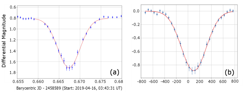
After the normal CCD image calibration including dark frame subtraction and flat fielding, we created light curves using airmass-corrected differential photometry. Both HS 2231+2441 and HS0705+6700 are typical of HW Vir-like eclipsing systems, their light curves show a strong reflection effect with a very deep primary and a shallow secondary minimum. We fit a Gaussian profile to the primary eclipse light curve using a nonlinear least-squares (Levenberg-Marquardt) algorithm and determine the observed mid-eclipse times. A sample light curve for HW Vir with associated Gaussian profile fit is shown in Fig. 1. We evaluated the uncertainty in time of eclipse minimum by a Monte Carlo method consisting of a series synthetic eclipse light curves with randomly-chosen times of minima and different exposure times. This procedure is described in detail in Appendix 1. Table 2 lists the eclipse timing observations and uncertainties for all three PCEBs.
3 Data Analysis
3.1 Data selection
Our eclipse timing dataset compromised 90 new time of primary eclipse minima (Table 2) together with previously published times from the literature. Before use, we made a few modifications.
-
1.
For HW Vir and HS2231+2441, we excluded a portion of archival SuperWASP times of minima that were rejected by Lohr et al. (2014)’s outlier methodology and by the size of their uncertainties. In particular, we did not include Lohr et al. (2014)’s listed extra times of minima due to their precision, and discarded timing data for which uncertainties are between 8 sec 40 sec. We also omitted the individual superWASP times of minima for HS2231+2441, since they had large () uncertainties.
-
2.
We also removed O-C eclipse timings obtained from the Mercator observation in Baran et al. (2018) for HW Vir since they deviate from the overall O-C trend line by 50 seconds. We also excluded outliers that had O-C values deviating by more than 400 seconds from the overall O-C trend.
3.2 Light Travel Time Model
For a binary system with orbiting substellar components, the predicted primary mid-eclipse time as a function of cycle number can be written as
| (1) |
where is the reference epoch, is the linear eclipse period, where are the time-dependent contributions from each perturbing body. and
| (2) |
is a quadratic term can would result from non-planetary effects, such as apsidal motion, mass exchange, magnetic braking, or gravitational radiation. We used the usual formulation of Irwin (1952, 1959) to calculate the time signature of perturbing bodies on eclipse timing as a function of each body’s orbital properties.
3.3 Orbit stability
A physically credible model must not only fit all the current and previously published ETV datasets, but it is also subject to the prior constraint that the substellar components must be stable to orbital instabilities over timescales at least comparable to the lifetime of the PCEB phase ( 100 Myr) (Han et al., 2002; Han et al., 2003; Zorotovic et al., 2011). We used the Hill stability criterion (Gladman, 1993; Chambers et al., 1996) to predict whether any two components in orbit about a massive central body will avoid mutual close encounters over many orbits.
For circular orbits, stability occurs if the semi-major axis difference between pairs of components exceeds a critical distance given by (Chambers et al., 1996),
| (3) |
where is the Hill radius,
| (4) |
where and are the masses and semi-major axes of the components respectively, and is the mass of the central body.
For non-circular orbits, a more general stability criterion is (Hasegawa & Nakazawa, 1990)
| (5) |
where
| (6) |
and is the larger eccentricity. For low eccentricity orbits and , we can expand the second term to obtain
| (7) |
The second term in parentheses is much less than 1 for the components considered here () so the simpler expression equation 3 was used in our calculations.
We can define a dimensionless parameter that characterizes each planet pair spacing in terms of the normalized mutual Hill radii as (cf. Smullen et al., 2016)
| (8) |
Stable component pairs correspond to while unstable pairs have .
For systems with more than two substellar components, instability can occur even if all components lie outside the Hill radius of their nearest companion, although the timescale for close encounters increases as the initial component separations become larger (Chambers et al., 1996). Hence, we used the Hill parameter as an optimization prior but ran numerical orbit simulations to test orbit stability after optimization, as described below.
3.4 Model Fitting Scheme
The model fitting scheme comprised four steps (Fig. 3):
-
1.
Create an initial model of between one and four sub-stellar components, with multi-component models spaced at least one Hill radius apart (i.e., for all pairs),
-
2.
Search for the minimum of an objective function proportional to the product of the summed of the model vs. O-C time series and an ansatz ’penalty’ function that sharply increases when the smallest Hill parameter becomes less than 1.0 for any component pair,
-
3.
Use Bayesian inference to solve for the final fitted parameters using a Markov chain Monte Carlo (MCMC) sampling, a weighted least-squares objective function, and an orbit stability prior (),
- 4.
We first chose the number of substellar companions to model. Examination of the O-C plot for both HS0705+6700 and HW Virginis indicates that a large number of components, although certainly possible, is not justified by the data, since the model parameters are already highly degenerate for few component models, as we will see. Hence we restrict our model selection to one through four component models. Each component is characterized by five parameters: mass, semi-major axis, eccentricity, longitude of periapsis , and time of periastron passage . We restricted the model to co-planar orbits for the sake of computational simplicity. We also added a period derivative parameter to account for the possible contribution of non-orbiting components, such as apsidal motion or gravitational radiation.
We started model fitting using a downhill simplex (Nelder-Mead) minimization (Python library LMFIT333https://lmfit.github.io/lmfit-py to fit the O-C curve. However, instead of minimizing the sum-squared differences between the O-C data and the model, we incorporate the orbit stability constraint by minimizing the product,
| (9) |
Where we define an empirical Hill stability function
| (10) |
where the Hill parameter is the smallest normalized Hill parameter (equation 8) of all component pairs. This stability function asymptotes to unity for but increases sharply for (see Fig.2).


The resulting model was used as a starting point for Bayesian inference modeling. We used the EMCEE (Foreman-Mackey et al., 2013) Python implementation444https://github.com/dfm/emcee with 4096 walkers and 4000 iterations. The likelihood function was summed-squared difference between the model and O-C data weighted by the data uncertainties. We used three priors: (i) stability parameter , (ii) all masses and semi-major axes positive-definite, and (iii) eccentricities restricted to the range .
Using a model fitting scheme with a Bayesian methodology as the final step has two important advantages over the more commonly-used frequentist least-squares minimization approach. First, the orbit stability constraint (Hill parameter) can be incorporated naturally as a Bayesian prior without the ad hoc ansatz function we used in the LMFIT minimization. Second, the Bayesian posterior distribution provides a more comprehensive description of the parameter uncertainties and correlations.
For each model, we tested dynamical stability by numerically integrating the component orbits using WHFAST, a Wisdom-Holman symplectic integrator (Rein & Tamayo, 2015). We used a time step of 36.5 days and integrated for 10 Myr for each model. In addition, we tested for chaotic behavior using the MEGNO algorithm (Mean Exponential Growth factor of Nearby Orbits, Cincotta & Simó (2000)) also with a time interval of 10 Myr. Both WHFAST and MEGNO were called from the Python package REBOUND (Rein & Liu, 2012) which also provided convenient tools for plotting orbits and time histories of orbital elements.
4 Results
4.1 HS2231+2441
After adding 26 additional primary eclipse timing observations (listed in Table 2) to previously published observations, we fit the linear ephemeris of Almeida et al. (2017) with a slightly changed orbital period,
| (11) |
The O-C diagram with all of the available data is shown in Figure 4.
We find that there is no statistically significant period variation for HS22315+2441 spanning 16 years, from 2004 to 2020, but we cannot rule out the variations smaller than 15 seconds. A linear fit without a orbiting planet is consistent with the full data set.

4.2 HS0705+6700


Figure 5 Shows the O-C timing residuals versus epoch computed using linear ephemeris,
| (12) |
along with our one component model (solid blue line) and the one-component model of Bogensberger et al. 2017 (solid green line). Table 4 lists the model parameters of our model.
We also found a best-fit two component model with masses 21.8 MJup and 1 MJup and semi-major axes 4.9 AU and 37.3 AU, respectively. The two component model was stable for at least years as verified by REBOUND and MEGNO simulations, but the fit to the timing data was no better than the one component model. Therefore, we do not discuss this model further.
It is clear that the previously published model of Bogensberger et al. deviates strongly from the observed timing data starting shortly after the publication of the model. As previously noted, this discouraging trend has been seen for several other eclipsing sdB binary exoplanet detection. Also, we did not plot the recent two component solution proposed by Sale et al. (2020) since we could not determine their ephemeris or interpret orbital parameters of their model from their paper.
An expanded view of the O-C fits for our model is shown in Fig. 6, along with the posterior spread from the EMCEE solutions. Fig. 7 shows the two-dimensional projections of the sample covariances for our one component model. They demonstrate that our model have well-defined parameters with small fractional uncertainties.
| Parameter | Fitted Values | Unit | |
|---|---|---|---|
| Inner Binary | |||
| T0 | 2451822.760509 | BJD | |
| P0 | 0.095646609 | day | |
| s/s | |||
| Substellar Component | |||
| yr | |||
| sec | |||
| AU | |||
| radian | |||
| Min. Mass | MJup | ||
| day | |||
4.3 HW Virginis

Figure 8 Shows the O-C timing residuals versus epoch using the linear ephemeris
| (13) |
On the right of each panel are plots of eccentricity and semi-major axes of all model components vs. epoch as computed by numerical integration using REBOUND with time steps of 0.1 yr. The plots also show two model fits:
-
•
The upper panel shows a three component model computed using the minimization scheme described in section 3, with a Bayesian prior for all component pairs, where is the normalized Hill constraint. This solution is stable for at least 10 Myr, but is a very poor fit to the timing data ().
-
•
The lower panel shows a 4-component model, also computed using the minimization scheme in section 3, but without the Hill stability prior. This provides a much better fit () but is highly unstable over short time internals (one hundred years).
We do not list the orbital elements for either model since they are implausible: They are either very poor fits to the timing data (3-component stable model) or are highly unstable (four-component model). This unfortunate scenario (acceptable O-C model fits are invariably unstable) was also found by (Brown-Sevilla et al., 2021) who analyzed a series of best-fit six multi-component models for HW Vir. In the next section we consider possible alternatives to pure substellar component models.
5 Alternative explanations for eclipse timing variations
As mentioned previously, eclipse timing variations can be caused by mechanisms other than gravitational perturbation by orbiting circumbinary masses. These include interbinary mass transfer, apsidal motion, and changes in the moment of inertia caused by magnetic activity on one of the components (Applegate mechanism).
For sdB binaries, mass transfer is ruled out since they are detached systems. Apsidal precession can result from (general relativistic) gravitational radiation and by tidal effects caused by an asymmetric mass distribution in one (or both) components. Lee et al. (2009) has shown that gravitational radiation for the sdB binary HW Vir, and by extension other similar systems including HS0705+6700, would result in time variations at about 2 dex smaller than observed.
Ruling out apsidal effects is more problematic since they depend on the tidal distortion of the internal mass distribution (via the internal structure constant , Sirotkin & Kim 2009) which is not well-characterized for these systems. Almeida et al. (2020) recently considered tidal and rotation apsidal effects on eclipse timing variations for the PCEB GK Vir, They found that apsidal is less likely than substellar component model, but could not rule it out as a contributing factor. In addition, apsidal effects will produce strictly periodic signatures in O-C plots, which is not observed for the binaries considered in this paper. Hence, we do not consider apsidal effects further, but examine the possible contribution of Applegate-type mechanisms.
Applegate (Applegate & Patterson, 1987; Applegate, 1992) proposed that orbital period changes in close binaries may result from a variable quadrupole moment produced by magnetic activity in the outer convection zone of one of the stars. For sdB binaries, this is likely to be the low-mass secondary, which is fully convective. Although we are not aware of any direct evidence for magnetic fields in any sdB secondary star, there is ample evidence for strong (kiloGauss) surface fields in many late-type (M0-M5) main sequence single stars similar to the secondaries in sdB binaries (e.g., Kochukhov, 2020, and references therein). Also, tidal locking will ensure that the rotation of the secondary is very rapid, enhancing the prospects for a robust magnetic dynamo.
The original Applegate mechanism assumed a time-dependent gravitational quadrupole moment modulated by the magnetic activity cycle in an outer thin shell of the active star. An increasing quadrupole moment results in a stronger gravitational field, driving a decreasing orbital radius and consequent reduction of the binary period. However, it was subsequently found that energy required to drive quadrupole moment variations of the secondary star that could account for the ETV’s was inconsistent with observed luminosity changes in many close binaries (Völschow, M. et al., 2016).
Several recent papers have analyzed modifications to the original Applegate model using more complex 2-shell models, generalizing the magnetohydrodynamic effects of internal magnetic fields, and considering different types of dynamo models (e.g., Lanza et al., 1998; Lanza, 2006; Navarrete, F. H. et al., 2018; Völschow, M. et al., 2018; Navarrete et al., 2019). Here we consider the recent model of Lanza (2020) which is based on angular momentum exchange between the spin of the active component and the orbital motion. Spin–orbit coupling is produced by a non-axisymmetric component of the gravitational quadrupole moment of the active star caused by an assumed persistent non-axisymmetric internal magnetic field.
5.1 Hybrid models with substellar components and Applegate-type modulation
As we have seen, the best-fit stable orbit model fits for both HS0705 and HW Vir are not fully in agreement with the observed O-C data, with residual average differences of order 10 sec and 20 sec over 10-20 year timescales for HS0705 and HW Vir respectively (Figs. 5,8). We now consider the question of whether the ETV variations may result from a combination of substellar component perturbation and Applegate-Lanza effects.
The change in fractional angular velocity of the secondary is related to the observed fractional period changes by (Lanza, 2020, eqn. 56)
| (14) |
Where in the reduced mass of the binary, is the semi-major axis of the binary, is the moment of inertia about the active (secondary) star spin axis, and is the fractional change in the period, or equivalently the O-C deviations over the timescale of the O-C data . The consequent change in rotational energy is
| (15) |
Combining these equations, the dependence on cancels, giving,
| (16) |
For both HS0705+6700 and HW Vir, the average timing residuals of the substellar companion model fits to the observed O-C data are both of order 10 sec over 10 yr (), while the bracketed term evaluates to J, so the change in rotational energy is
| (17) |
We can compare this with the maximum energy available from luminosity changes over the timescale for O-C variability in the secondary star. From Table 3,
| (18) |
Remarkably, this is the same as the energy loss required to account for residual changes in the O-C model fits, but would be only of the entire O-C deviations from a constant period were due to an Applegate-Lanza mechanism. This suggests that the observed O-C variations could be explained by a combination of substellar companions accounting for the bulk of the ETV’s, with a Lanza-Applegate mechanism contributing about 10% of the total.
5.2 Tidal Synchronization Timescale
Another relevant dynamical timescale is the tidal synchronization time i.e., the timescale in which tides on the secondary dissipate the kinetic energy of asynchronous rotation (Lanza, 2020),
| (19) |
where Q is a dimensionless tidal quality factor that characterizes the efficiency of tidal energy dissipation in the active (secondary) component, is the total mass of the binary system, is the primary mass, is the binary semi-major axis, and is the active star radius. Following Lanza (2020), we assume corresponding to strong tidal coupling due to nearly synchronous rotation. For the moment of inertia , we use the numerical expression of Criss & Hofmeister (2015) for a fully convective secondary star with a polytropic index n = 1.5,
| (20) |
Using stellar parameters list in Table 3, we find tidal synchronization timescales = 4 – 40 yr and 10 – 100 yr for HS0705 and HW Vir respectively. These times are comparable to the observed O-C variations, so tidal synchronization may dictate the timescale for spin-orbit coupling rather than magnetic activity timescales.
6 Summary and Conclusions
In this paper, we have reported new eclipse timing observations of three post-common envelope binary systems. We combined these observations with previously published timing data to investigate whether the eclipse timing variations from a linear ephemeris could be explained by the gravitational influence of orbiting substellar companions. We used models comprising multiple substellar companions in coplanar orbits parallel to the observer’s line of sight, adjusting their orbital parameters and masses to best fit the observed timing variations.
For one of the three binaries (HS2231+2441), nearly all times of minima are consistent with a linear ephemeris. Hence, there is no evidence for substellar companions in this system, although they cannot be ruled out if the masses are small. However for the remaining two binaries, there are large timing variations (ETV) from the linear trend, indicating the presence of one or more gravitationally perturbing effects. We focused on finding orbital parameters and masses of companions that could account for the observed ETV’s by varying the masses and orbital elements to best-fit the observed ETV time signature using a least-squares minimization.
In order to ensure that the substellar components had stable orbits, the minimization function included a Hill stability ‘penalty’ ansatz that increases sharply when the minimum separation between adjacent components was smaller than one Hill radius. We also used a Bayesian inference algorithm to better characterize the uncertainties of the derived orbital parameters and masses. In addition, we used the Hill stability criterion as a prior to restrict orbital solutions only to those that were plausibly long-term stable i.e., at least as long as the assumed time scale for common-envelope evolution (Schreiber & Gänsicke, 2003; Ivanova et al., 2013).
Finally, we checked stability timescales for each model using a numerical N-body symplectic time-step integrator (WHFAST) and an algorithm to detect the onset of chaotic behavior (MEGNO). We ran both the numerical integrations and chaos indicator time evolutions for years.
For HS0705+6700, we found one and two-component models that reasonably reproduced the observed ETV time history and were stable on long time scales ( yr). However, the fits were not statistically convincing, with reduced chi-squares of the fitted models in the range 10–19, although this may be partly a result of underestimated uncertainties in previously published timing measurements (cf. Hinse et al., 2014).
For HW Vir, we found no stable solutions that could fit the ETV time signature, although it was possible to find adequate four component fits, albeit with highly unstable orbits. This has also been the conclusion of several previous studies of HW Vir (e.g., Horner et al., 2012; Brown-Sevilla et al., 2021) and although not definitive, this strongly suggests that substellar companions cannot account for all of the ETV time history observed in these (and likely other) PCEB binaries.
Therefore, we investigated whether some fraction of the observed variations could be caused by an Applegate mechanism in which the secondary star’s gravitational quadrupole moment is altered by magnetic activity. Although the original Applegate mechanism was found to be energetically insufficient to account for the observed timing variations in sdB binaries (e.g., Völschow, M. et al. 2016), various revisions of the mechanism have been suggested that may account for at least a fraction of the observed variations.
We applied the model of Lanza (2020), in which spin–orbit coupling is produced by an active (secondary) star’s non-axisymmetric internal magnetic field creates a non-axisymmetric gravitational quadrupole moment. Using this model, we find that the predicted timing variations could account for perhaps 10% of the observed O-C variability, although this result is uncertain, since it is dependent on poorly constrained binary system parameters such as the tidal energy dissipation and the internal mass distribution of the stars. Hence, we posit that the observed O-C variations could result from a hybrid model in which substellar companions account for a largest fraction of the timing variations, but that an Appleget-Lanza mechanism contributes the remainder.
Acknowledgements
This research made use of the LMFIT nonlinear least-square minimization Python library, and Astropy, a community developed core Python package for Astronomy. We also made use of emcee, an MIT licensed pure-Python implementation of the affine invariant Markov chain Monte Carlo (MCMC) ensemble sampler (Goodman & Weare, 2010). We also used the excellent Python module corner.py to visualize multidimensional results of Markov Chain Monte Carlo simulations (Foreman-Mackey, 2016). Numerical orbit integrations in this paper made use of the REBOUND N-body code (Rein & Liu, 2012). The simulations were integrated using WHFAST, a Wisdom-Holman symplectic integrator (Rein & Tamayo, 2015).
We are grateful to David Pulley, John Mallett and the Altair Group for their contribution of times of minima for HS0705+6700 on Dec 29th, 2019, and times of minima for HW Vir on June 6th, 2019. We are also grateful to Prof. Antonino Lanza for several very insightful communications. The Iowa Robotic Observatory is funded by the College of Liberal Arts at the University of Iowa.
Data Availability
We have provided Table 2 as our new mid-eclipse timing data of three post-common envelope binaries. The light curves available on request from the corresponding author.
References
- Almeida et al. (2017) Almeida L. A., Damineli A., Rodrigues C. V., Pereira M. G., Jablonski F., 2017, MNRAS, 472, 3093
- Almeida et al. (2020) Almeida L. A., Pereira E. S., Borges G. M., Damineli A., Michtchenko T. A., Viswanathan G. M., 2020, Monthly Notices of the Royal Astronomical Society, 497, 4022
- Applegate (1992) Applegate J. H., 1992, ApJ, 385, 621
- Applegate & Patterson (1987) Applegate J. H., Patterson J., 1987, ApJ, 322, L99
- Baran et al. (2018) Baran A. S., et al., 2018, MNRAS, 481, 2721
- Bear & Soker (2014) Bear E., Soker N., 2014, Monthly Notices of the Royal Astronomical Society, 444, 1698
- Beuermann et al. (2012a) Beuermann K., et al., 2012a, A&A, 540, A8
- Beuermann et al. (2012b) Beuermann K., Dreizler S., Hessman F. V., Deller J., 2012b, A&A, 543, A138
- Bogensberger et al. (2017) Bogensberger D., Clarke F., Lynas-Gray A. E., 2017, Open Astronomy, 26, 134
- Brown-Sevilla et al. (2021) Brown-Sevilla S. B., et al., 2021, Monthly Notices of the Royal Astronomical Society, 506, 2122
- Carter et al. (2008) Carter J. A., Yee J. C., Eastman J., Gaudi B. S., Winn J. N., 2008, The Astrophysical Journal, 689, 499
- Chambers et al. (1996) Chambers J., Wetherill G., Boss A., 1996, Icarus, 119, 261
- Cincotta & Simó (2000) Cincotta P. M., Simó C., 2000, Astron. Astrophys. Suppl. Ser., 147, 205
- Criss & Hofmeister (2015) Criss R. E., Hofmeister A. M., 2015, New Astron., 36, 26
- Deeg (2021) Deeg H. J., 2021, Galaxies, 9
- Deeg, H. J. (2015) Deeg, H. J. 2015, A&A, 578, A17
- Drechsel et al. (2001) Drechsel H., et al., 2001, A&A, 379, 893
- Esmer et al. (2021) Esmer E. M., Baştürk Ö., Hinse T. C., Selam S. O., Correia A. C. M., 2021, A&A, 648, A85
- Foreman-Mackey (2016) Foreman-Mackey D., 2016, Journal of Open Source Software, 1, 24
- Foreman-Mackey et al. (2013) Foreman-Mackey D., Hogg D. W., Lang D., Goodman J., 2013, PASP, 125, 306
- Gladman (1993) Gladman B., 1993, Icarus, 106, 247
- Goodman & Weare (2010) Goodman J., Weare J., 2010, Communications in Applied Mathematics and Computational Science, 5, 65
- Han et al. (2002) Han Z., Podsiadlowski P., Maxted P. F. L., Marsh T. R., Ivanova N., 2002, MNRAS, 336, 449
- Han et al. (2003) Han Z., Podsiadlowski P., Maxted P. F. L., Marsh T. R., 2003, Monthly Notices of the Royal Astronomical Society, 341, 669
- Hasegawa & Nakazawa (1990) Hasegawa M., Nakazawa K., 1990, A&A, 227, 619
- Heber (2009) Heber U., 2009, Annual Review of Astronomy and Astrophysics, 47, 211
- Heber (2016) Heber U., 2016, Publications of the Astronomical Society of the Pacific, 128, 082001
- Hinse et al. (2010) Hinse T. C., Christou A. A., Alvarellos J. L. A., Goździewski K., 2010, MNRAS, 404, 837
- Hinse et al. (2014) Hinse T. C., Horner J., Lee J. W., Wittenmyer R. A., Lee C.-U., Park J.-H., Marshall J. P., 2014, A&A, 565, A104
- Horner et al. (2012) Horner J., Hinse T. C., Wittenmyer R. A., Marshall J. P., Tinney C. G., 2012, MNRAS, 427, 2812
- Horner et al. (2014) Horner J., Wittenmyer R., Hinse T., Marshall J., Mustill A., 2014, Wobbling Ancient Binaries - Here Be Planets? (arXiv:1401.6742)
- İbanoǧlu et al. (2004) İbanoǧlu C., Çakırlı Ö., Ta\textcommabelows G., Evren S., 2004, A&A, 414, 1043
- Icko & Livio (1993) Icko J. I., Livio M., 1993, Publications of the Astronomical Society of the Pacific, 105, 1373
- Irwin (1952) Irwin J. B., 1952, ApJ, 116, 211
- Irwin (1959) Irwin J. B., 1959, AJ, 64, 149
- Ivanova et al. (2013) Ivanova N., et al., 2013, A&ARv, 21, 59
- Kilkenny et al. (1994) Kilkenny D., Marang F., Menzies J. W., 1994, MNRAS, 267, 535
- Kilkenny et al. (2000) Kilkenny D., Keuris S., Marang F., Roberts G., van Wyk F., Ogloza W., 2000, The Observatory, 120, 48
- Kilkenny et al. (2003) Kilkenny D., van Wyk F., Marang F., 2003, The Observatory, 123, 31
- Kiss et al. (2000) Kiss L. L., Csák B., Szatmáry K., Furész G., Sziládi K., 2000, A&A, 364, 199
- Kochukhov (2020) Kochukhov O., 2020, The Astronomy and Astrophysics Review, 29, 1
- Kwee & van Woerden (1956) Kwee K. K., van Woerden H., 1956, Bull. Astron. Inst. Netherlands, 12, 327
- Lanza (2006) Lanza A. F., 2006, MNRAS, 369, 1773
- Lanza (2020) Lanza A. F., 2020, MNRAS, 491, 1820
- Lanza et al. (1998) Lanza A. F., Rodono M., Rosner R., 1998, MNRAS, 296, 893
- Lee et al. (2009) Lee J. W., Kim S.-L., Kim C.-H., Koch R. H., Lee C.-U., Kim H.-I., Park J.-H., 2009, The Astronomical Journal, 137, 3181
- Lohr et al. (2014) Lohr M. E., et al., 2014, A&A, 566, A128
- Marsh (2018) Marsh T. R., 2018, Circumbinary Planets Around Evolved Stars. Springer International Publishing, Cham, pp 2731–2747, doi:10.1007/978-3-319-55333-7_96, https://doi.org/10.1007/978-3-319-55333-7_96
- Martin (2018) Martin D. V., 2018, Populations of Planets in Multiple Star Systems. Springer International Publishing, Cham, pp 2035–2060, doi:10.1007/978-3-319-55333-7_156, https://doi.org/10.1007/978-3-319-55333-7_156
- Mayor & Queloz (1995) Mayor M., Queloz D., 1995, Nature, 378, 355
- Nasiroglu et al. (2017) Nasiroglu I., et al., 2017, AJ, 153, 137
- Navarrete, F. H. et al. (2018) Navarrete, F. H. Schleicher, D. R. G. Zamponi Fuentealba, J. Völschow, M. 2018, A&A, 615, A81
- Navarrete et al. (2019) Navarrete F. H., Schleicher D. R. G., Käpylä P. J., Schober J., Völschow M., Mennickent R. E., 2019, Monthly Notices of the Royal Astronomical Society, 491, 1043
- Nebot Gómez-Morán et al. (2011) Nebot Gómez-Morán A., Gänsicke B. T., Schreiber M. R., Schwope A. D., 2011, in Schmidtobreick L., Schreiber M. R., Tappert C., eds, Astronomical Society of the Pacific Conference Series Vol. 447, Evolution of Compact Binaries. p. 187
- Østensen et al. (2007) Østensen R., Oreiro R., Drechsel H., Heber U., Baran A., Pigulski A., 2007, in Napiwotzki R., Burleigh M. R., eds, Astronomical Society of the Pacific Conference Series Vol. 372, 15th European Workshop on White Dwarfs. p. 483
- Parsons et al. (2013) Parsons S. G., et al., 2013, Monthly Notices of the Royal Astronomical Society: Letters, 438, L91
- Pulley et al. (2015) Pulley D., Faillace G., Smith D., Watkins A., Owen C., 2015, Journal of the British Astronomical Association, 125, 284
- Pulley et al. (2018) Pulley D., Faillace G., Smith D., Watkins A., von Harrach S., 2018, A&A, 611, A48
- Qian et al. (2008) Qian S.-B., Dai Z., Zhu L.-Y., Liu L., He J.-J., Liao W.-P., Li a., 2008, The Astrophysical Journal Letters, 689, L49
- Qian et al. (2009) Qian S.-B., et al., 2009, The Astrophysical Journal, 695, L163
- Qian et al. (2010) Qian S. B., et al., 2010, Ap&SS, 329, 113
- Qian et al. (2013) Qian S. B., et al., 2013, MNRAS, 436, 1408
- Rein & Liu (2012) Rein H., Liu S. F., 2012, A&A, 537, A128
- Rein & Spiegel (2015) Rein H., Spiegel D. S., 2015, MNRAS, 446, 1424
- Rein & Tamayo (2015) Rein H., Tamayo D., 2015, MNRAS, 452, 376
- Sale et al. (2020) Sale O., Bogensberger D., Clarke F., Lynas-Gray A. E., 2020, Monthly Notices of the Royal Astronomical Society, 499, 3071
- Schleicher & Dreizler (2014) Schleicher D. R. G., Dreizler S., 2014, A&A, 563, A61
- Schleicher et al. (2015) Schleicher D. R. G., Dreizler S., Völschow M., Banerjee R., Hessman F. V., 2015, Astronomische Nachrichten, 336, 458
- Schreiber & Gänsicke (2003) Schreiber M. R., Gänsicke B. T., 2003, A&A, 406, 305
- Schwarz et al. (2016) Schwarz R., Funk B., Zechner R., Bazsó Ã., 2016, Monthly Notices of the Royal Astronomical Society, 460, 3598
- Shakura (1985) Shakura N. I., 1985, Soviet Astronomy Letters, 11, 224
- Sirotkin & Kim (2009) Sirotkin F. V., Kim W.-T., 2009, The Astrophysical Journal, 698, 715
- Skelton (2012) Skelton P. L., 2012, African Skies, 16, 132
- Smullen et al. (2016) Smullen R. A., Kratter K. M., Shannon A., 2016, MNRAS, 461, 1288
- Tokovinin (2014) Tokovinin A., 2014, The Astronomical Journal, 147, 87
- Völschow, M. et al. (2016) Völschow, M. Schleicher, D. R. G. Perdelwitz, V. Banerjee, R. 2016, A&A, 587, A34
- Völschow, M. et al. (2018) Völschow, M. Schleicher, D. R. G. Banerjee, R. Schmitt, J. H. M. M. 2018, A&A, 620, A42
- Webbink (1984) Webbink R. F., 1984, ApJ, 277, 355
- Wittenmyer et al. (2012) Wittenmyer R. A., Horner J., Marshall J. P., Butters O. W., Tinney C. G., 2012, Monthly Notices of the Royal Astronomical Society, 419, 3258
- Wittenmyer et al. (2013) Wittenmyer R. A., Horner J., Marshall J. P., 2013, Monthly Notices of the Royal Astronomical Society, 431, 2150
- Wolszczan & Frail (1992) Wolszczan A., Frail D. A., 1992, Nature, 355, 145
- Zorotovic & Schreiber (2013) Zorotovic M., Schreiber M. R., 2013, A&A, 549, A95
- Zorotovic et al. (2010) Zorotovic M., Schreiber, M. R. Gänsicke, B. T. Nebot Gómez-Morán, A. 2010, A&A, 520, A86
- Zorotovic et al. (2011) Zorotovic M., Schreiber M. R., Gänsicke B. T., 2011, Astronomy & Astrophysics, 536, A42
- Çakirli & Devlen (1999) Çakirli Ö., Devlen A., 1999, A&AS, 136, 27
Appendix A Time of minimum Uncertainty estimates
In this appendix, we evaluate the uncertainty in the time of minimum determination of an eclipsing binary light curve constructed from a series of images with relatively long exposure times and image download times. These pertain especially to observations using relatively small-aperture telescopes, including those reported in this paper.
A standard technique used by many previous authors (more than 1,100 citation!) is the folded-symmetry algorithm described by Kwee & van Woerden (1956). This technique determines the time of minimum by adjusting a trial midpoint time and minimizing the summed squared magnitude difference between points equally time-displaced on either side of the midpoint. The associated uncertainty is determined by fitting a quadratic function and applying standard propagation of errors to fitted minimum value. The technique relies on equally-space data samples and does not account for interpolation errors when this is not the case. Other more sophisticated methods (e.g., Carter et al., 2008; Deeg, H. J., 2015; Deeg, 2021) have addressed eclipse timing uncertainty, but they generally have been restricted to trapezoidal light curves, as observed in exoplanet transits. This is not applicable to short-period binary systems, whose eclipse light curves are much closer to Gaussian profiles (e.g., Baran et al., 2018).
We evaluated time of minimum uncertainty using a Monte Carlo approach, simulating observed eclipse light curves with a Gaussian profile whose width, depth, and scatter closely resembles the observed light curve. Fig. 9 shows a light curve of HS0705+6700 observed on with the Iowa Robotic telescope, along with the corresponding simulated light curve. The synthetic light curve was made by sampling a Gaussian function with 0.25 magnitude eclipse depth, and 300 sec half-width. We added Gaussian random noise to each sampled point, with a standard deviation where is the differential magnitude difference to the out-of-eclipse level. The synthetic light curve was sampled every 10 msec. We then binned the simulated date into 40 second bins with 10 second time gap between bins, corresponding the the observed image exposure time and download times for HS0705+6700. The magnitude assigned to each image was the computed mean value of 10 msec samples within each bin. The resulting synthetic light curve was fit with a Gaussian profile to determine the time of minimum. This process was repeated 10,00 times with different times of minima varying from -100 sec to +100 sec relative to the nominal zero-point time of minimum. The difference between the true time of minimum and the fitted time of minimum was recorded.
A histogram of the time difference between the best-fit time of minimum and the true minimum for 1,000 realizations is shown in Fig.10. The width is 4 seconds.
