Early-stage Resource Estimation from
Functional Reliability
Specifications in
Embedded Cyber-Physical Systems
Abstract
Reliability and fault tolerance are critical attributes of embedded cyber-physical systems that require a high safety-integrity level. For such systems, the use of formal functional safety specifications has been strongly advocated in most industrial safety standards, but reliability and fault tolerance have traditionally been treated as platform issues. We believe that addressing reliability and fault tolerance at the functional safety level widens the scope for resource optimization, targeting those functionalities that are safety-critical, rather than the entire platform. Moreover, for software based control functionalities, temporal redundancies have become just as important as replication of physical resources, and such redundancies can be modeled at the functional specification level. The ability to formally model functional reliability at a specification level enables early estimation of physical resources and computation bandwidth requirements. In this paper we propose, for the first time, a resource estimation methodology from a formal functional safety specification augmented by reliability annotations. The proposed reliability specification is overlaid on the safety-critical functional specification and our methodology extracts a constraint satisfaction problem for determining the optimal set of resources for meeting the reliability target for the safety-critical behaviors. We use SMT (Satisfiability Modulo Theories) / ILP (Integer Linear Programming) solvers at the back end to solve the optimization problem, and demonstrate the feasibility of our methodology on a Satellite Launch Vehicle Navigation, Guidance and Control (NGC) System.
Keywords Formal Specification, Resource Allocation, Processor Minimization
1 Introduction
With increasing dependence of safety-critical systems on software and embedded computing, the notions of reliability and fault tolerance have undergone a paradigm shift. While the traditional approach for enhancing reliability in electro-mechanical systems is based on replication of physical components [21, 24, 32, 39, 3, 30], safety-critical embedded cyber-physical systems (CPS) must also consider reliability of software executions, packet drops in networks, priority inversion in scheduling of control tasks on shared processors, and many other factors which are attributed to the computational platform which executes the cyber part of the system [7, 28].
In the domain of cyber-physical systems, reliability targets of embedded control can be met through fault-tolerant design of the underlying platform and its structural components or through fault-tolerant deployment of the control software on the underlying platform. The former looks at the necessary resource requirements for providing reliable service at the platform level without specific focus on individual control components [4]. For example, while designing the CAN matrix for an automobile, we choose the topology and number of CAN segments depending on the overall loading of the buses and the reliability concerns thereof. On the other hand, fault-tolerant deployment of control focuses on individual control tasks [15]. For example, it includes replication of software tasks on multiple cores [38] and sometimes on the same core (temporal redundancy) [14, 26, 23, 25], or provides fault-tolerant scheduling frameworks that involve cloning of a sequence of tasks for layered task graphs [10, 37]. Fault-tolerant deployment also influences the choice of the platform and its components, but with respect to the reliability requirements for individual functional components.
The design cycle of cyber-physical systems begin with the preparation of a specification of the functionalities of the system. The use of formal specifications for defining the functional safety properties of such systems has been widely recommended in most industrial standards, including aeronautics (DO-178C), automotive (ISO 26262), industrial process automation (IEC 61508), nuclear (IEC 60880), railway (EN 50128) and space (ECSS-Q-ST-80C), specifically for those functionalities that require a high safety-integrity level. Although reliability and fault tolerance are as important attributes of the system design as functional correctness [6, 8, 9, 11, 27, 34], or performance attributes such as timing [1, 2, 12, 13, 33], power [17, 18] and security [22], formal specification of reliability, especially with respect to the critical functional safety properties has so far received very little attention. This is largely due to the perception that reliability and fault tolerance need to be addressed at the platform level, not at the functional level [20, 40]. On the other hand, we believe that with the increasing cost of electronics and software in cyber-physical systems, investment on reliability needs to be prioritized on the basis of the safety-criticality of the system’s functions.
This paper presents, for the first time, a methodology for overlaying formal functional safety specifications with reliability annotations and estimating the resource requirement from such extended specifications. A formal specification enables the designer to lay out the strategy for redundant computations and/or actuations [16] and obtain a formal reliability guarantee for the strategy using the proposed method of analysis. Moreover since this is done at the specification level, our methodology provides early estimates of the resource requirements, thereby facilitating design space exploration, where the tradeoff between reliability and resource requirements can be studied using the proposed methodology until an acceptable balance is achieved.
In particular, our previous work [16] explores various reliable strategies enabled by the given reliability specifications and converges on a strategy that maximizes the reliability – thereby also pointing out whether the specified reliability targets are attainable for every functionality of the design. In our level of abstraction, an action represents a discrete control event which is enabled by a logically defined pre-condition (sense) and achieves a logically specified consequent (outcome) when executed successfully on the underlying computational platform. We use the term action-strategy to denote possible sequences of actions that lead to some desired outcome. An action-strategy is admissible with respect to a reliability target, if the sequence and timing of actions involved in that strategy guarantees the desired outcome with the specified reliability guarantee. It may be noted that, more than one admissible action-strategies may exist for a functionality and every participating action (at any time instant) in an admissible strategy requires one processor (computing resource) to execute.
In the early stage of design of a complex, multi-component embedded control system, the designer must plan the sense-control-actuation steps for each control loop along with the corresponding timing constraints. The formal safety specification at this stage defines the necessary outcomes of the closed loop system as a timed function of the sensed input events. For example, we may be given a safety property of the form:
where sense_A is a sense event and outcome_B is the desired outcome which must happen within the time interval [1:10] following the sense event. Now in order to ensure that outcome_B does actually happen in that window of time, the control system must perform appropriate actions (called actuations).
Suppose we have an action, called action_C which can cause outcome_B, but the causality is not fully guaranteed. Suppose:
which means that action_C, if used, can cause outcome_B 80% of the time. Now suppose our reliability target for the above safety property is . If the sense event, sense_A, triggers one execution of the action, action_C, then the reliability with which outcome_B is guaranteed is only . Therefore, in order to achieve the target of , we must be prepared to repeat action_C more than once, either on different resources, or on the same resource but at different times. Moreover, all executions must be completed within the specified window of time, namely [1:10], following the event sense_A.
In a complex system, there can be many safety properties and therefore, many different actions may have to be repeated spatially and/or temporally to achieve the desired reliability. We provide a framework, where the system designer can overlay a chosen pattern of redundancy over the temporal fabric of the safety specification. For example, consider the following specification:
The above specification specifies that following a sense_A event, the action, action_C, will be executed in parallel at some time in the window [2:5], and will be again executed after units of time. It be noted that all three executions of action_C are constrained by time windows, but they can be executed in more than one way within the specified windows. A formal specification framework like this has two immediate advantages:
-
1.
We can verify whether the specified redundancy in the executions of the actions achieves the target reliability of the safety properties.
-
2.
Each possible schedules of the actions provides us an early estimate of the resource requirements. We can also find the schedule which has the optimal resource requirement. In a complex system, with many actions and replications, this is a non-trivial task and computationally beyond manual capacity.
It may also be noted that two admissible action-strategies with respect to two different reliability specifications may share some common actions. Given a set of admissible action-strategies with respect to various sensed-events, it is necessary to predict the amount of resources (processors) required in order to execute all of them in a worst-case scenario when all sensed-events, take place together. This estimation is non-trivial due to the sharing of actions and the redundancy provisions present in the strategies, and hence the choice of an appropriate admissible action-strategy with respect to every sensing is a key to reduce the number of resources. This paper presents a novel technique for selecting and grouping the set of admissible action-strategies attributed from various specifications with respect to different sensed-events, so that the number of resources needed in the worst case for executing the actions is minimized.
With the rapid growth in the number of features supported in modern appliances, the computing paradigm is shifting from a federated architecture where each feature runs on a dedicated processor to an integrated architecture where Electronic Control Units (ECUs) are shared among multiple features. While integrated architectures are able to reduce the costs of electronics and networking, the scheduling and fault tolerant deployment of control tasks has become more complex. We believe that having an early estimate of the resource requirements, as in the proposed approach, can help in taking rational decisions on the tradeoff between reliability and resource costs.
Our early work, presented in [16], introduces the formal framework for reliability specification. The problem of estimating resource requirements from such specifications is treated in this paper for the first time. The main contributions of this paper are as follows:
-
•
We extract all possible admissible reliability strategies from a given reliability specification, that meets the desired reliability target for a functional specification.
-
•
We formulate the resource optimization problem in terms of a constraint-satisfaction problem which can be solved using SMT / ILP solvers.
-
•
We have studied the proposed technique over test-cases from automotive domain and also shown the scalability of our approach over several experiments.
-
•
We illustrate the practicality of our proposed technique using a case-study (over Satellite Launch Vehicle Navigation, Guidance and Control (NGC) System) from avionics domain.
It is important to note that resource estimation is intricately related to the code volumes associated with the control tasks and their worst case execution times (WCET) on the chosen ECUs. In practice, the design of embedded systems is a process that goes through multiple generations of a product, and statistical knowledge about the execution times and the probability of their success in terms of providing the desired outcome are available from legacy data. Therefore early estimation of the tradeoff between functional reliability and resource requirements is feasible in practice, though not in established practice today.
The paper is organized as follows. Section 2 illustrates the preliminary concepts and the earlier works carried out to set up the premise for this work. In Section 3, we present the formal problem definition and methods to determine the optimal number of resources. The experimental results showing the efficacy of our proposed framework is given in Section 4. In Section 5, we demonstrate our proposed methodology using a practical case-study. Finally, Section 6 concludes the paper with a brief discussion on the ramifications of the proposed approach.
2 Background Work and Preliminaries
An embedded controller of a CPS comprises of three primary modules, namely Sensor, Controller and Actuator – which interacts with the Plant (or the environment) to perform desired behaviors. The sensor is responsible for sensing input scenarios from the plant (or the environment). The controller performs the control decision based on the sensed input. The actuator delivers actuation signals to the plant (or the environment). Some of the activities in CPS control may be implemented using software and the rest may be controlled via hardware. For example, sensing a scenario where the brake should be applied automatically, the computation of appropriate brake-pressure may be carried out using a software program. However, maintaining the same break-pressure for a certain amount of time is performed by a hardware-control. The resultant outcome while applying such actions is the application of the wheel-brakes and thereby reduction in the vehicle speed. We present a formal model for embedded CPS and such requirements in the following.
Figure 1 provides a schematic representation of the embedded CPS framework. Here, the events that are responsible for sensing inputs, actions (actuations) and outcome activities are termed as sensed-events (), action-events () and outcome-events (), respectively. While interacting with the plant model, the controller receives the sensed-events and compute appropriate actions/actuations to produce the desired outcome-events. The outcome of an action may take place after many control cycles and may also be durable over a period of time. Typically, the control software execution platform is responsible to compute appropriate actuations for the desired outcomes being enabled.
The reliability of the CPS is governed by the fault-free execution from sensed to the outcome events. This intuitively means, after sensing an input scenario, how reliably an action (actuations) can be performed once the controller decision is undertaken properly. In this model, the reliability of the outcome activities are attributed from the unreliable computational platform where the action events are scheduled, computed and applied. To meet the desired reliability of the outcome behavior, the fine-grain control incorporates various physical redundancy attributes in the scheduled actions inside the control execution platform. It may be noted that the unreliability lies primarily in the execution of action-events (as per our model), though there can also be failures in the sensing and application of outcome activities or imperfections in message communications. However, this framework can be suitably extended to handle such uncertainties in other components of the embedded CPS framework.
From an abstract point of view, the activities of a CPS can be visualized in terms of sequence of events. The early-stage functional specification narrates the outcome-event based on a sensed scenario which is to be met with specific reliability targets. Such specifications describe the correctness requirements for a CPS. In addition to this, the meta-level action-strategy specifies the supervisory control orchestrated by the control software where the redundancies in actions are described for a sensed scenario. Such requirements are termed as CPS reliability specifications [16].
Now, let us revisit the formal model for such embedded CPS specifications as introduced in [16] using an elementary correctness requirement, , for the subsystem, , with a sense-event, , and an outcome-event, as follows:
It means that, whenever is sensed then the outcome-event is asserted within next to time-units111The formal expressions of the properties have syntactic (and semantic) similarity with SystemVerilog Assertions (SVA) [42].. Suppose, is the action-event responsible for producing the outcome . If the probability of success for given the successful execution of is expressed as, , then the current reliability () of the property, , is also . Since we have , so happens under the assumption of a perfect sense and action scenario222We assume that the control system senses perfectly (without any false positives or false negatives) and also generates appropriate actions based on the sensed-event., where both and .
At the design-level, the controller can leverage spatial and temporal redundancy provisions to improve the reliability of the outcome-events and thereby enhance the functional reliability of the design specifications. Figure 2(a) and Figure 2(b) show the schematic models where the spatial and temporal redundancy provisions are incorporated at the controller level. In the spacial redundancy model for a CPS control system, , there are parallel instances of the controller, namely and computational counterparts, . The controllers sense the same events () and produce the action-events (), respectively, at time . Each action-event goes into a possibly unreliable computational counterpart, , respectively. On the other hand, in the temporal redundancy model, number of re-executions are made by a single controller within the time-window from to . At time (), the controller, , senses same input-event, , and produces the action-event, . This action-event goes into the possibly unreliable computational counterparts, , and produces an output-event at . Finally, the outcome-event, , produces successful (correct) outcome if one of the outputs of (or ) produces correct result for both these cases333We assume a fail-silent model here, where failure in any outcome implies discontinuation of that outcome – thereby it will not interfere with other correct outcomes and can possibly be distinguished from these correct outcomes..
Such design-level redundancy provisions can be captured from the functional specification-level as well. For example, we can formally represent the spatial and temporal redundancies (as shown in Figure 2) using the properties, and , respectively, as follows:
Here, asserts that, whenever is sensed then the action-event is asserted parallelly in execution units (denoted by the construct) within next to time-units. Similarly, asserts that, whenever is sensed then the action-event is asserted times by multiple executions (denoted by the construct) within next to time-units. At this current setup, the reliability of the outcomes are also increased and these are represented as, and , respectively.
Let us present an example to explain such functional correctness and reliability specifications.
Example 1
Adaptive Cruise Control (ACC) supports features to – (a) maintain a minimum following interval to a lead vehicle in the same lane and (b) control the vehicle speed whenever any lead obstacle is present. Let us consider the functional requirements of ACC, which senses the proximity of any lead vehicle and a leading obstacle by the sense-events, and , respectively. The required action-events issued by the ACC controller for reducing throttle by and applying proper pressure in wheel-brakes are denoted as, and , respectively. The corresponding outcome-events are given as, and . It may be noted that a single time-unit delay is considered to be of ms in all the functional specifications mentioned below.
Now, consider the following two functional correctness requirements of ACC as follows:
-
(a)
: As soon as a lead obstacle is sensed, then within a total of ms, the throttle is adjusted (reduced by ) followed by the application of wheel brakes after - ms. Formally, this property is expressed as:
-
(b)
: Whenever a lead vehicle is sensed in a close proximity, then within a total of ms, the throttle is adjusted (reduced by ) followed by the application of wheel brakes after - ms. Formally, this property is expressed as:
Suppose, the desired reliability of the given correctness requirements be and for and , respectively. Here, the actions and are responsible for producing the outcome-events and , respectively. Suppose, the outcome-events are unreliable and their reliability values are given as:
Since the outcomes are unreliable, the ACC must issue the action-events with appropriate redundancy in order to meet the desired reliability target, as given by the following reliability specifications.
-
(a)
: As soon as a lead obstacle is sensed, then the throttle-reduction action-event is scheduled in two processors parallelly within ms, followed by the brake-apply action-event which is also scheduled in two processors parallelly within next ms. Formally, this property is expressed as:
-
(b)
: Whenever a lead vehicle is sensed in a close proximity, then the overall action of throttle-reduction applied successively twice, followed by brake-application in the next time-unit is re-executed twice within an overall time limit of ms. Formally, this property is expressed as:
Now, given the reliability specifications, and and assuming that the sensed-events ( and ) are present in Cycle-0, the reliability for the correctness specifications, and are calculated in Table 1 and Table 2, respectively, with respect to each action/control strategy444The method for formal reliability assessment is presented in [16] in details.. For example, the reliability computed from Option- in Table 1 is given as, , since there are spatial redundancy provisions for each action in with respect to the outcomes of . Similarly, the reliability computed from Option- in Table 2 is given as, , since there are ways to satisfy from the given action-strategy of .
| Possible | Action Events (Cycle-wise) | Computed | |||
| Options | Cycle-1 | Cycle-2 | Cycle-3 | Cycle-4 | Reliability |
| (1A) | |||||
| (1B) | |||||
| (1C) | |||||
| (1D) | |||||
| Possible | Action Events (Cycle-wise) | Computed | |||||
| Options | Cycle-1 | Cycle-2 | Cycle-3 | Cycle-4 | Cycle-5 | Cycle-6 | Reliability |
| (2A) | |||||||
| (2B) | |||||||
| (2C) | |||||||
| (2D) | |||||||
| (2E) | |||||||
| (2F) | |||||||
3 Reliability-aware Resource Estimation
In this section, we formally present the problem of reliability-aware resource estimation and illustrate the detailed resource allocation procedure.
3.1 Formal Statement of the Problem
The problem of finding the optimal number of computing resources (processors) considering the simultaneous occurrences of a set of sensed-events is formally described as:
Given:
-
(i)
A set of formal correctness and reliability properties of the system,
-
(ii)
Assigned reliability targets with respect to each correctness specification,
-
(iii)
The set of sensed-events that may occur simultaneously, and
-
(iv)
A set of admissible action-strategies corresponding to every sensed-event (derived from the corresponding reliability properties of the system).
Objective: To determine the appropriate choice of action-strategy with respect to every sensed-event so that the overall resource/processor requirement is minimized.
Assumptions:
-
(i)
Same actions participating under two different action-strategies corresponding to different sensed-events can be executed together in the same processor.
-
(ii)
Execution of every action takes unit time (one cycle) in the processor.
-
(iii)
Within one action-strategy, the participating actions appear as disjunction-free.
Assumption-(i) prevents this resource optimization problem to have similar behavior as any conventional two-dimensional strip packing problems [31] and hence we cannot directly apply those solutions here. However, the solution space is determined by several possible choices of the action-strategy combinations attributing to the varied number of processors required. The following example illustrated this in details.
Example 2
Let us revisit Example 1 where we derive the admissible action-strategies for the two specifications of subsystem in the highlighted rows of Table 1 and Table 2.
Suppose, the sensed-events, and , occur simultaneously at Cycle-0. Then, Table 3 denotes possible execution options for the action-events combining the both the strategies. For example, if we try to ascertain Options with , then we need two processors in Cycle-1 to execute two parallel events among which one event of Option is shared/paired with the from Option .
| Strategy | Possible Executions of Action-Events (Cycle-wise) | Resource | ||||
| Comb. | Cycle-1 | Cycle-2 | Cycle-3 | Cycle-4 | Cycle-5 | Req. |
| 1A+2A | ||||||
| 1A+2B | ||||||
| 1A+2D | ||||||
| 1B+2A | ||||||
| 1B+2B | ||||||
| 1B+2D | ||||||
| 1C+2A | ||||||
| 1C+2B | ||||||
| 1C+2D | ||||||
| 1D+2A | ||||||
| 1D+2B | ||||||
| 1D+2D | ||||||
Such action sharing helps us to reduce the number of processor requirements. We find that combination requires processors to execute the action strategies. Table 3 presents all the possible combinations and the required resources while executing each of these combinations of action strategies. It may be noted that, the minimum number of resources () is required when we perform the actions as per the Options and for both the properties. Hence, the next challenge is to bind the action-events with respect to Cycles so that the required resources are minimized.
3.2 Resource Estimation Procedure
The required number of resources can be computed from a set of admissible action-strategies (corresponding to sensed-events) derived from the reliability properties of a system, assuming that the corresponding set of sensed-events occur simultaneously. The minimum count of execution units depends on the optimal allocation of the actions to appropriate processor cores in every execution time/cycle so as to maximize the sharing of action executions. The entire problem can be modeled as a Constraint Satisfaction Problem (CSP) which can be solved by an SMT / ILP solver.
Figure 3 illustrates the primary steps in this framework. The steps that are involved here are primarily categorized in two broad parts, namely – 1. Parsing and Action Representation and 2. Constraint Generation.
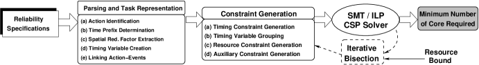
1. Parsing and Action Representation
From the reliability properties and the derived action-strategies, the first step is to identify relevant information of the action-event occurrences, their timing and redundancy related information so that the required constraints can be derived later. We present various stages of parsing and action representation as follows.
-
(a)
Action Identification: This step identifies the set of action-events from reliability specifications. For reliability specifications having redundant actions, duplicate action-events are created.
-
(b)
Time Prefix Determination: The time prefix of an action-event, extracted from the reliability specification, is typically given as either (fixed-time) or (time-range) where , the set of all non-negative integers. The lower and upper bound of the time prefixes are represented using a doublet, , for the fixed time prefix and a doublet, , for representing the variable time prefix. The redundancies are treated as follows:
-
•
In case of spatial redundancy (-times), all replicated actions (from to occurrences) have as the time-prefix.
-
•
In case of temporal redundancy (-times), let the time prefix for the first action in the first execution be extracted as . Then, the first action of () re-executed sequence can start earliest at and latest by 555 is computed from the reliability specification considering the given reliability target of the corresponding correctness property. Intuitively, this upper bound in time comes from the fact that delaying the start (beyond ) in re-executing the same sequence reduces the number of possible satisfaction of the correctness property and hence the specified reliability remains unmet (Literature [16] provides more details). – thereby having as the time-prefix. The time prefixes of the other actions are extracted from the specification and remain same across all their re-executions.
-
•
-
(c)
Spatial Redundancy Factor Extraction: Action-events with spatial redundancy of are represented by associating each replication with a spatial redundancy factor from to . A default spatial redundancy factor of is assigned to action-events having no spatial redundancy.
-
(d)
Timing Variable Creation: Timing variable represents the time of occurrence of an action-event. For every action-event identified from the reliability properties, unique timing variables are created for each occurrence (replicated or re-executed) of that action, which will be used to derive the constraints relating to the time of execution of these action-events.
-
(e)
Linking Action-Events: For every action-event appearing in the reliability specification, the timing-related constraints will be generated either from the absolute time of its occurrence or in relative to the timing of its preceding event. Hence, we need to map each timing variable (corresponding to an action-event) to the timing variable of its preceding action – thereby aiding to the generation of timing constraints for action-event sequences with respect to an action-strategy. The first action-event in the reliability specification is not linked to any other events, since it depends only on the time of occurrence of the sensed-event. Hence, the timing variable corresponding to the first action-event has its linked variable as . For redundancies, the action-event links are done as follows:
-
•
In case of spatial redundancy (-times), all replicated actions (from to occurrences) are linked with the first occurrence of that action.
-
•
In case of temporal redundancy (-times), the first action in the re-execution () is linked with the first action in the re-execution.
-
•
These stages of parsing and action representation are illustrated in details through Example 3.
Example 3
Consider the reliability specifications, and , with their corresponding correctness specifications, and , as given in Example 1.
| Action | Time Pref. | Sp.-Red. Factor | Time Var. | Link Var. |
|---|---|---|---|---|
| is computed from w.r.t. the reliability targets of | ||||
| Action | Time Pref. | Sp.-Red. Factor | Time Var. | Link Var. |
|---|---|---|---|---|
2. Constraint Generation
Primarily, the set of generated constraints can be of the following two types – (i) timing-related constraints, and (ii) resource-related constraints. However, the detailed stages, needed to derive these constraints to be used by the CSP solver, are given below.
-
(a)
Timing Constraint Generation: Given a reliability specification, , let the timing variable corresponding to an action, , be . It has the time-prefix and is linked with another action, , having the timing variable as (). Then, the timing constraints for are,
(1) If , then the timing constraint is simplified as,
(2) -
(b)
Timing Variable Grouping:
Timing variable are grouped to enable resource minimization through its sharing. Variables corresponding to same action are grouped together and corresponding to every action, at least one group is formed. Given two reliability specifications, and , having a common action, , let the timing variables corresponding to , be and , respectively. Then, we can put and together forming one group, , i.e., . It may be noted that, all the timing variables belonging to one group, say , are associated with the same action-event, say , from different properties. Here, can also be the first occurrence of an action being replicated -times (spatial redundancy).
Moreover, in case of spatial redundancy (say, action in is replicated -times), the timing variables, , corresponding to every replicated action ( to occurrence) forms a singleton group, i.e., . Now, if exists in another specification, , with spatial redundancy -times, then the grouping varies, depending on the relative values of and :
-
•
If , then .
-
•
If , then and singleton groups, .
-
•
-
(c)
Resource Constraint Generation: Pairing of timing variables into groups helps us to generate resource constraints such that, if then the corresponding actions (say, from and from ) are same, i.e. . So, these actions can be executed once whenever possible – resulting in a reduction in the execution resources (processors). Let an action-event, executing at cycle-, be represented using the timing variable ; then the required resource due to the execution of only that action is given as,
The number of resources required at - by the group of timing variables representing an action is denoted as,
Suppose we are given with specifications, , , , . We choose all timing variables belonging to each () from the group,
and create sub-groups of as,
Now, the required resource count for each of these sub-groups, , is denoted as,
The sub-group count indicates the number of coincident action-events belonging to the same specification (implied by temporal redundancy). Hence, we indicate the total number of resources required at - to execute the actions from these n sub-groups of as,
Let all the timing variables corresponding to the action-event, , appear in groups, , , , . Then, we define,
A pertinent point to note here is that, for a group, , if there is no temporal redundancy involved (in the specification) for the representative action of that group, then we find, and the required resources at - becomes, . Hence, the generated resource constraint for - is derived as follows:
(3) -
(d)
Auxiliary Constraint Addition: Two types of auxiliary (additional) constraints are derived to make the constraint generation process complete. These are discussed below.
-
•
Admissibility Constraint: We have noticed in Section 2 that, among all the action-strategies that are generated from a reliability specification with respect to the given reliability target of its corresponding correctness property, there is a subset of action-strategies which are admissible. Let us assume that the last execution of an action-event can happen latest at - such that all action-strategies remain admissible. Then, we need to add a constraint with respect to the timing variable, , corresponding to the last executed action as,
-
•
Resource Limit Constraint: We start with a pessimistic bound on the number of resources required and gradually refine that limit. For a given choice of maximum number of resources, , these constraints are expressed as,
-
•
All these generated constraints can also be used in a constraint optimization tool/solver (like ILP solvers). There, we need to add the additional objective function providing the minimization or maximization requirement. Since we are minimizing the number of resources (processors) in this case, the objective function will be:
Example 4
-
•
Timing Constraints: The timing constraints with respect to the property, , are derived as:
Similarly, the timing constraints with respect to the property, , are derived as:
Now, is extracted from the logical satisfaction of using subject to specific reliability targets.
-
•
Timing Variable Groups: The timing variables for each action-events is grouped as follows:
Here, all the timing variables present in the groups and correspond to action-event and that are present in the groups and correspond to action-event.
-
•
Resource Constraints: The resource constraints are derived using Table 5 for each -. Finally, we produce the following constraints ():
Table 5: Resource Constraint Generation (for -) Groups -
•
Auxiliary Constraints: The admissibility constraint, here, restricts the last action-event, , to happen latest by -cycle, i.e. (Refer to Table 4 of Example 3 for admissible action-strategies). Hence, we add, .
Suppose, we set the resource limits as , then the added constraints are as follows:
If we fed all the above constraints together in a SMT/ILP solver, then we find the following satisfiable valuation of the variables:
It indicates that, both and of is replicated twice in - and -, respectively. Two consecutive followed by of is executed for the first time in -, - and -, respectively. Again, re-execution of the same sequence happens when two consecutive followed by is executed for the second time in -, - and -, respectively. This result is also evident from Example 3, where the choice of Options produces this outcome as shown in Table 3.
The resource constraints and the timing constraints are fed together to a SMT solver to check the satisfiability. If these constraints can be satisfied, then we conclude that the given resource limit, , is sufficient for the admissible action strategies to be scheduled. However, an unsatisfiable outcome denotes that the resource limit needs further increment. To solve this using an ILP solver, we also add the objective constraint (for minimization).
Now, to derive the optimal (minimum) number of required resources, we start from a pessimistic limit and proceed on iteratively bisecting the limit (in a similar manner as done in binary search technique) until we converge into finding the minimum value of the resource limit. To illustrate the procedure, let us assume that we start with a given in our example and derive the satisfiable valuations. Then, we bisect the limit and make and still we can derive satisfiable valuations as illustrated in Example 4. Next, when we further bisect and make , then the constraints become unsatisfiable. Hence, we conclude that the minimum number of resources required to execute the admissible strategies is .
4 Experimental Results
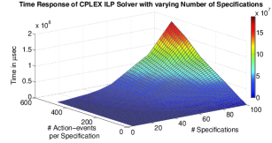
In this section, the experimental results performed to check the scalability of this approach on an -Core Intel Xeon Ivy bridge series processor ( Cache, ) with RAM are presented. Figure 4 and 5 shows the 3D plots on the scalability experiments performed. We have used Z3 SMT solver [36] developed by Microsoft Corporation and CPLEX Optimizer (ILP solver) [19] developed by IBM. The time response of the proposed approach subject to varying sequential depth666The sequential depth of a property is the maximum number of cycles throughout which the property may span. and number of action-events were analyzed. The graphs depict exponential increase in execution time in determining the optimal resources as the sequential depth of the specifications increase. The time response with varying number of properties and varying number of action-events per property are also studied. This response also has exponential behavior as indicated in Figures 4-5.
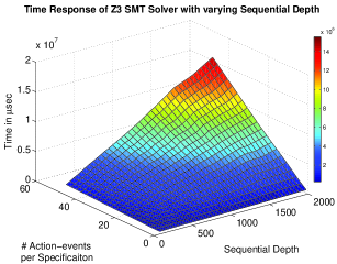
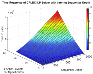
In Figure 4, the responses of Z3 and CPLEX solvers are shown with respect to the variations in sequential depth of the properties. The Z-axis in all the graphs represents the time required to find the minimum number of resources in Micro-seconds. The X-axis indicates the sequential depth (varied upto time units) and the Y-axis indicates the number of action-events in the specification (varied upto ). For smaller sequential depth, the variation in execution time with variation in the number of action-events is rather small. However, as the sequential depth increases, the execution time varies rapidly as the number of action-events increases. The increases in sequential depth also results in the increase in number of resource constraints. Moreover, the increase in number of action-events results in increase in the length and complexity of resource constraints as well. But for same number of action events, the number of timing constraints remains the same. The increase in number of resource constraints has higher impact in the increase of execution time than the increase in the length of resource constraints.
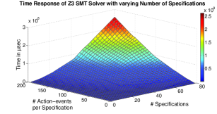
In Figure 5, the response of Z3 and CPLEX solvers are shown with respect to the variations in the number of specifications. The Z-axis in all the graphs represents the time required to find the minimum number of resources in Micro-seconds. The X-axis indicates the number of specifications (varied from to /) and the Y-axis indicates the number of action-events per specification (varied upto /). For smaller number of specifications, the variation in the execution time with the variation in number of action-events is rather small. However, as the number of specifications increases, the execution time varies rapidly. Here, the increase along the X-axis and Y-axis results in increase in the number of timing constraints. This increase in number of timing constraints can result in increase of the number of action-events and the number of specifications. There will be variation in the number of resource constraints, implied by both increase in the number of action-events as well as in the number of properties, since time of execution can vary in both these cases. Both X-axis and Y-axis has similar effects in increasing the length and number of resource constraints. Thus, the behavior is truly exponential in this case. The increase in timing constraints have lesser effect on the time of execution than the increase in the length/complexity of the resource constraints.
Comparison of Results obtained by Constraint Solvers (Z3 and CPLEX)
It may be noted that, when modeling our resource estimation problem as a Constraint Satisfaction Problem (CSP) or a Constraint Optimization Problem (COP), there are two types of constraints to be considered. The first type is the timing constraints that define definite timing relationship between the action-events constituting the feasible action-event strategies meeting specific reliability targets. The second type is the resource constraint, this restraint is to be kept on all viable time value or the maximum depth of time over which the action strategy can exist assuming the sensed-event corresponding to the reliability specifications happens at time zero.
Both the solvers, Z3 (CSP solver) [36] and CPLEX (ILP/COP solver) [19] will share the same timing and resource constraints. However, ILP requires an objective function to be provided in addition to the constraints presented to Z3777In general, the objective function is either a cost function or energy function which is to be minimized, or a reward function or utility function, which is to be maximized.. We can check the satisfiability of the given set of reliability specifications with respect to any specific number of cores using Z3 [5]. In CPLEX, the objective function is defined as the sum of the number of time cycles where the resource constraints are met and maximization of the same can result in the optimal satisfiable solution to the problem [35]. Hence, we are finding an assignment that maximizes the number of satisfied resource constraints in ILP to model the problem.
Comparing the performance of the Z3 solver with the CPLEX solver, the CPLEX is significantly faster in both scenarios. The primary reason behind this behavior is the fact that CPLEX ILP solver is a COP solver [29]. The search space of the ILP solver is limited to the optimal hyper-plane which maximizes the objective function and hence the ILP solver will be faster in reaching the minimum number of resources. The calculation of the optimal plane offsets the difference slightly, still there is an appreciable variation in execution time between two solvers.
5 Case-Study: Navigation, Guidance and Control (NGC) System for Satellite Launch Vehicles
The satellite launch vehicle navigation, guidance and control (NGC) system is responsible for directing the propulsive forces and stabilizing the vehicle to achieve the orbit with the specified accuracy. The dispersions in propulsion parameters compared to expected values, variations of the estimated aerodynamic characteristics during the atmospheric flight phase, the fluctuating winds both at ground and upper atmosphere and a variety of internal and external disturbances during the flight can increase the loads on the vehicle beyond the permissible limit and also cause deviations in the vehicle trajectory from its intended path [41]. Under such environment, NGC system has to define the optimum trajectory in real time to reach the specified target and steer the vehicle along the desired path and inject the spacecraft into the mission targeted orbit within the specified dispersions while ensuring the vehicle loads remain within limits. NGC system is among the most crucial and challenging field in launch vehicle design. The objectives of a satellite launch vehicle NGC system include:
-
1.
Stabilization of the vehicle during its flight against various disturbance forces and moments due to aerodynamics, thrust misalignment, separation, liquid slosh, etc.
-
2.
Tracking the desired attitude of the vehicle so as to follow the desired trajectory with the specified accuracy to meet the final mission objectives.
-
3.
Receiving navigation data from sensors (navigation sensors) and desired attitude from guidance system and generating appropriate control commands.
Using the control commands generated by the autopilot system, the actuation system generates the necessary forces and moments to control and stabilize the vehicle as per the requirements. The inputs to the launch vehicle autopilot system are – navigation sensor data and health status, guidance data and health status, sequencing command execution status, feedback from vehicle autopilot filters, and feedback from Autopilot on the status of computation and validation.
5.1 Correctness Specifications
The list of correctness specifications888It is to be noted that a single time-unit delay is considered to be of ms in all the above mentioned correctness specifications. for NGC system are expressed formally as follows:
-
(1)
: If the system detects permanent navigation sensor failure in all channels, then the system will discard navigation sensor data within - ms, followed by switching to open loop guidance within - ms and then initialize the salvage profile for control within - ms.
-
(2)
: If the system detects permanent failure in one of the navigation sensor channels, then the system discards failed channel within - ms, followed by recalculation of navigation parameters from redundant channels within - ms.
-
(3)
: If the system detects off-nominal navigation parameters from navigation software and the navigation sensors being healthy, then the system discards present parameters within - ms, followed by recalculation of navigation parameters within - ms.
-
(4)
: If the system detects guidance algorithm failure, then the system will discard present guidance computations within - ms, followed by switching to open loop guidance within - ms, followed by salvage profile initialization for control within - ms.
-
(5)
: If the system detects off-nominal values for one of the guidance parameters with the guidance algorithm being healthy, then the system discards and flushes out the present computation within ms, followed by recalculation within - ms.
-
(6)
: If the system detects error in the execution of vehicle autopilot commands, then the system switches to open loop guidance within - ms, followed by salvage profile initialization for control within - ms.
-
(7)
: If the system detects any failure in switching Vehicle Autopilot digital filters, then the system switches to open loop guidance within - ms, followed by salvage profile initialization for control within - ms.
-
(8)
: If the system detects non-execution of sequencing(time-based) commands for the first time, then the system re-schedule time-based commands within - ms, followed by rechecking the execution status within - ms.
-
(9)
: If the system detects non-execution of sequencing(time-based) commands more than once, then the system will switch to open loop guidance within - ms.
-
(10)
: If the system detects error in on board arithmetic computation unit, then the system discards all computations within - ms, followed by switching to open loop guidance within -ms, followed by salvage profile initialization for control within -ms.
-
(11)
: If the system detects off-normal control parameters with the control algorithm being healthy then the system will recalculate guidance parameters within - ms, followed by the recalculation of control parameters within ms.
-
(12)
: If the system detects any communication error between navigation, guidance, control or sequencing then the system will switch to open loop guidance within - ms, followed by salvage profile initialization for control within - ms.
-
(13)
: If the system detects temporary failure in any of the navigation sensor channels then the system will discard sensor data within - ms, followed by the recalculation of navigation parameters using the redundant channels within ms.
-
(14)
: If the system has any temporary failure reported in any of the navigation sensor channels then the system will recheck the particular channel values for re-induction within - ms.
-
(15)
: If the system detects any timing failure due to shift in clock frequency then the system will discards all computations within - ms, followed by switching to open loop guidance within - ms, followed by salvage profile initialization for control within - ms.
5.2 Reliability Specifications
Table 6 outlines various activities of NGC system and the corresponding outcome-events responsible for that. Also, the respective action-events for each outcome event and the reliability values for the outcomes, i.e. , are specified.
| Event Description | Outcome-Event | Action-Event | Reliability Values |
|---|---|---|---|
| switching to open loop guidance | |||
| initialization of salvage profile for control | |||
| discarding error channel | |||
| recalculation of navigation parameters | |||
| discarding previous navigation parameters | |||
| discarding present computations | |||
| rescheduling sequencing commands | |||
| rechecking sequencing command execution status | |||
| recalculating control parameters | |||
| discarding sensor data | |||
| rechecking error channel | |||
| recalculating guidance parameters |
In addition to this, let us assume that the desired reliability of all the given correctness requirements be . Since the outcomes are unreliable, the NGC system must issue the action-events with appropriate redundancy in order to meet the desired reliability target, as expressed formally by the following reliability specifications999It is to be noted that a single time-unit delay is considered to be of ms in all the above mentioned reliability specifications..
-
(1)
: As soon as the navigation sensor permanent failure is detected in all the channels, the navigation sensor data is discarded within - ms followed by scheduling the switching to open loop guidance action-event in two processors parallelly within - ms, followed by the salvage profile initialization action which is also scheduled in two processors parallelly within next - ms.
-
(2)
: As soon as the system detects permanent failure in one of the navigation sensor channels, system does the action corresponding to discarding failed channel within - ms followed by initiating the action to recalculate navigation parameters from redundant channels within - ms. The latter action is repeated consecutively twice.
-
(3)
: As soon as the system detects off-nominal navigation parameters from navigation software and the navigation sensors being healthy, system initiates action to discard present parameters within - ms followed by recalculation action to calculate navigation parameters within - ms. The second action is repeated consecutively twice.
-
(4)
: whenever the system detects guidance algorithm failure, system will perform action corresponding to discard present guidance computations within - ms followed by switching to open loop guidance action within - ms followed by salvage profile initialization for control within - ms. The latter two actions are repeated non-consecutively twice.
-
(5)
: whenever the system detects off-nominal values for one of the guidance parameters with the guidance algorithm being healthy, system does the action corresponding to discarding the present computation within ms followed by recalculation action within - ms.
-
(6)
: As soon as the system detects error in the execution of vehicle autopilot commands, then the system initiates the action to switch to open loop guidance within - msfollowed by salvage profile initialization action for control within - ms. Both the actions are spatially repeated twice.
-
(7)
: As soon as the system detects any failure in switching Vehicle Autopilot digital filters, then the overall action to switch to open loop guidance is scheduled within - ms followed by salvage profile initialization action for control is scheduled - ms, is repeated non-consecutively twice.
-
(8)
: If the system detects non-execution of sequencing(time-based) commands for the first time, system will do action corresponding to rescheduling of time-based commands within - ms followed by rechecking action to check the execution status within ms. The latter action is repeated non-consecutively twice.
-
(9)
: As soon as the system detects non-execution of sequencing(time-based) commands more than once, system will do action corresponding to switching to open loop guidance within ms non-consecutively twice.
-
(10)
: Whenever system detects error in on board arithmetic computation unit, system discards all computations within - ms followed by action to switch to open loop guidance is executed parallelly in two units within -ms followed by salvage profile initialization action for control is executed parallelly in two units within -ms.
-
(11)
: If the system detects off-normal control parameters with the control algorithm being healthy system will trigger action to recalculate guidance parameters within - ms followed by triggering action to recalculate control parameters within -ms. The second action is repeated in two parallel units.
-
(12)
: As soon as the system detects any communication error between navigation, guidance, control or sequencing, The system will repeat the overall action to switch to open loop guidance within - ms followed by salvage profile initialization for control within - ms, non-consecutively twice.
-
(13)
: If the system detects temporary failure in any of the navigation sensor channels system will do action to discard sensor data within - ms followed by the recalculation of navigation parameters is repeated consecutively twice using the redundant channels within -ms.
-
(14)
: whenever system has a temporary failure reported in any of the navigation sensor channels then system will do rechecking action to check the particular channel values for re-induction within - ms and is repeated non-consecutively twice.
-
(15)
: As soon as the system detects timing failure due to shift in clock frequency, system will discards all computations within - ms followed by switching to open loop guidance within ms followed by salvage profile initialization for control within - ms. The latter two actions are non-consecutively repeated twice.
5.3 Analysis and Discussion
| Possible | Action Events (Cycle-wise) | Computed | |||||||
| Options | Cycle-1 | Cycle-2 | Cycle-3 | Cycle-4 | Cycle-5 | Cycle-6 | Cycle-7 | Cycle-8 | Reliability |
| (4A) | |||||||||
| (4B) | |||||||||
| (4C) | |||||||||
| (4D) | |||||||||
| (4E) | |||||||||
| (4F) | |||||||||
| (4G) | |||||||||
| (4H) | |||||||||
| (4I) | |||||||||
| (4J) | |||||||||
| (4K) | |||||||||
| (4L) | |||||||||
| (4M) | |||||||||
| (4N) | |||||||||
| (4O) | |||||||||
| (4P) | |||||||||
| Possible | Action Events (Cycle-wise) | Computed | ||||||
| Options | Cycle-1 | Cycle-2 | Cycle-3 | Cycle-4 | Cycle-5 | Cycle-6 | Cycle-7 | Reliability |
| (13A) | ||||||||
| (13B) | ||||||||
| (13C) | ||||||||
| (13D) | ||||||||
| (13E) | ||||||||
| (13F) | ||||||||
| (13G) | ||||||||
| (13H) | ||||||||
Given the reliability specifications, and assuming that the sensed-events are present in , the reliability for the correctness specifications, can be calculated with respect to each action/control strategy, in the same way as shown in Example 1. We present two representative tables, namely Table 7 and Table 8, corresponding to the specifications, and , respectively, to demonstrate the result101010For brevity, we are not showing the tables for all specifications mentioned.. To illustrate the computation of reliability values, let us analyze one example action strategy, say , from Table 8 which is defined over the correctness specification, , and reliability specification, . Here, the realization of can happen in two possible ways as per : (i) followed by immediately in the next cycle; or (ii) followed by after a gap of one cycle. Since, it is given that and , therefore the computed reliability becomes, . The highlighted rows of Table 7 indicate the admissible action-strategies that meet the desired reliability requirements for the property, and , of subsystem. For example, Table 7 shows that the action strategies, and are admissible with computed reliability values , whereas options do not meet the desired reliability target.
Our proposed methodology analyzes the given specifications with reliability targets and searches for appropriate allocation of the action-events (cycle-wise) so that the minimum number of resources are required to realize the specifications. Table 9 shows the cycle-wise allocations for all the action-events (from the reliability specifications of NGC system) attributing to the minimum resource requirement, assuming simultaneous occurrence of all sensed-events. It may be noted that, here we need a minimum of three (3) resources to realize the given set of specifications, which is evident from the last column of Table 9.
| Reliability | Admissible Action | Action-event Allocation Schedule | ||||||
|---|---|---|---|---|---|---|---|---|
| Specification | Strategy Index | Cycle-1 | Cycle-2 | Cycle-3 | Cycle-4 | Cycle-5 | Cycle-6 | Cycle-7 |
| Action-event Allocation | ||||||||
| (cycle-wise) | ||||||||
Though the simultaneous occurrence of all sensed-events is the pessimistic-case and needs to be analyzed for deriving the worst-case resource requirements, but in practical scenarios, all the sensed-events may not appear simultaneously. If we assume that the only temporary failures (sensed-events corresponding to , , , , , and ) would happen simultaneously (failures which would not lead to the selection of salvage profile) and the remaining sensed-events (corresponding to , , , , , , and ) occurs or more cycles later, the number of resources required is only two (2) as shown in Tables 10 and Table 11. This is the minimum number of resources required, assuming all the sensed-events do not occur together.
| Reliability | Admissible Action | Action-event Allocation Schedule | ||||||
|---|---|---|---|---|---|---|---|---|
| Specification | Strategy Index | Cycle-1 | Cycle-2 | Cycle-3 | Cycle-4 | Cycle-5 | Cycle-6 | Cycle-7 |
| Action-event Allocation | ||||||||
| (cycle-wise) | ||||||||
| Reliability | Admissible Action | Action-event Allocation Schedule | ||||
|---|---|---|---|---|---|---|
| Specification | Strategy Index | Cycle-1 | Cycle-2 | Cycle-3 | Cycle-4 | Cycle-5 |
| Action-event Allocation (cycle-wise) | ||||||
In addition to this, we also provide Figure 6 and Figure 7 to show how our analysis time and the minimum resource requirements depend on the increase in temporal and spatial redundancy factors to improve reliability.
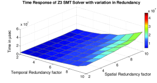
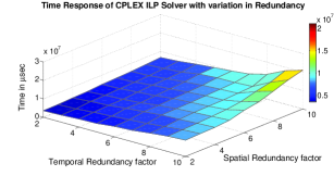
In Figure 6 the response of Z3 and CPLEX solvers to variations in number of specifications is shown. The Z-axis in the graphs represents the time required to find the minimum number of resources in Microseconds. Where as in Figure 7, the Z-axis indicates the resource requirement predicted by the algorithm. The X-axis indicates the spatial redundancy artifact incorporated in the reliability specifications (varied from to ) in all the graphs. The Y-axis indicates the temporal redundancy artifact incorporated in the reliability specifications (varied from to ) in all the graphs. As the redundancy incorporated increases, the execution time varies exponentially. Here the increase along the X-axis and Y-axis results in increase in number of timing constraints. This increase in number of timing constraints can be attributed to increase in number of action-events due to increased redundancy. There will be variation in number of resource constraints, implied by increase in number of action-events.
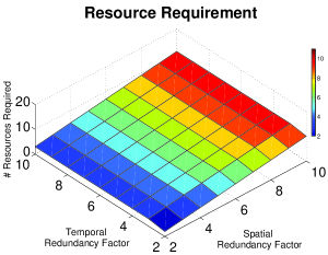
Comparing the performance of the Z3 solver with the CPLEX solver, the CPLEX is significantly faster in the above scenario. The CPLEX ILP solver being a COP solver, its search space is limited to the optimal hyper plane which maximizes the objective function making it more efficient. The resource requirement varies linearly as redundancy incorporated increases. The resource required is a linear function of incorporated redundancy.
6 Conclusion
Early-stage estimation of required resources from formal reliability specifications could be helpful in reducing the cost of a safety-critical system. This is typically decided at the design time of such systems and often the choice remain pessimistic by putting additional resources than required. In this work, we propose an algorithm to find the optimum number of processing resources required to guarantee the reliability target of given specifications. The problem is modeled as a Constraint Satisfaction Problem (CSP) or Constraint Optimization Problem (COP) which can be solved efficiently using an SMT solver or an ILP solver, respectively. Such an analysis is really helpful in safety-critical embedded system development. The practicality of the proposed method has been shown over the case-studies from automotive as well as avionics domain. Besides, the scalability experiments reveal the applicability and efficacy of the proposed method in complex systems.
The work presented here is an enabler for early prediction of computing resources in embedded CPS control systems based on their reliability requirements. However, it is pertinent to note that this work considers the sense, action and outcome of events from an abstract (specification) level of system design, and therefore we restrict ourselves without considering the communication delays between components and other details from this early design stages. Moreover, scheduling provisions of the action events is also kept as static in order to accurately specify the temporal boundaries in the specification. In future, we plan to extend the specification and analysis framework to incorporate more realistic communication delays and may also keep provisions for dynamic scheduling of the events. Such specification-level extensions will require much improved analysis involving the interference in component-level activities as well. In addition to this, along with the unreliable computational platform producing outcomes failures, ramifications due to the unreliable nature of sensed and action event generation also needs to be explored in future for completeness.
Acknowledgement
The authors thank Noel Philip (Quality Engineer, Systems Reliability Entity, VSSC-ISRO) for helping in developing the NGC subsystem case-study. Besides, P.P. Chakrabarti acknowledges the partial support from DST, India and P. Dasgupta acknowledges the partial support from FMSAFE project (under IMPRINT-India).
References
- [1] R. Alur and D. L. Dill. A Theory of Timed Automata. Theoretical Computer Science, 126(2):183–235, 1994.
- [2] R. Alur, A. Itai, R. P. Kurshan, and M. Yannakakis. Timing Verification by Successive Approximation. In Computer-Aided Verification (CAV), pages 137–150, 1992.
- [3] A. Avizienis and J. P. J. Kelly. Fault Tolerance by Design Diversity: Concepts and Experiments. IEEE Computers, 17(8):67–80, 1984.
- [4] M. Baleani, A. Ferrari, L. Mangeruca, A. L. Sangiovanni-Vincentelli, M. Peri, and S. Pezzini. Fault-tolerant Platforms for Automotive Safety-critical Applications. In Proceedings of the International Conference on Compilers, Architecture and Synthesis for Embedded Systems (CASES), pages 170–177, 2003.
- [5] C. W. Barrett, R. Sebastiani, S. A. Seshia, and C. Tinelli. Satisfiability Modulo Theories. Handbook of satisfiability, 185:825–885, 2009.
- [6] A. Biere, A. Cimatti, E. M. Clarke, and Y. Zhu. Symbolic Model Checking without BDDs. Lecture Notes in Computer Science, 1579:193–207, 1999.
- [7] S. Chakraborty, Md. A. Al-Faruque, W. Chang, D. Goswami, M. Wolf, and Q. Zhu. Automotive Cyber-Physical Systems: A Tutorial Introduction. IEEE Design & Test, 33(4):92–108, Aug. 2016.
- [8] E. M. Clake, A. Biere, R. Raimi, and Y. Zhu. Bounded Model Checking Using Satisfiability Solving. The Journal of Formal Methods in System Design, 19(1):7–34, 2001.
- [9] E. M. Clarke, O. Grumberg, and D. A. Peled. Model Checking. MIT Press, 2000.
- [10] D. Das, P. Dasgupta, and P. P. Das. A Heuristic for the Maximum Processor Requirement for Scheduling Layered Task Graphs with Cloning. Journal of Parallel and Distributed Computing, 49(2):169–181, 1998.
- [11] P. Dasgupta. A Roadmap for Formal Property Verification. Springer, 2006.
- [12] M. G. Dixit, P. Dasgupta, and S. Ramesh. Taming the Component Timing: A CBD Methodology for Real-time Embedded Systems. In Design Automation and Test in Europe (DATE), pages 1649–1652, 2010.
- [13] M. G. Dixit, S. Ramesh, and P. Dasgupta. Time-budgeting: A Component Based Development Methodology for Real-time Embedded Systems. Formal Aspects of Computing Journal, 26(3):591–621, 2014.
- [14] R. Geist, R. Raynolds, and J. Westall. Selection of a Checkpoint Interval in a Critical-Task Environment. IEEE Transactions on Reliability, 37(4):395–400, 1988.
- [15] D. Goswami, D. Müller-Gritschneder, T. Basten, U. Schlichtmann, and S. Chakraborty. Fault-tolerant Embedded Control Systems for Unreliable Hardware. In 2014 International Symposium on Integrated Circuits (ISIC), pages 464–467, 2014.
- [16] A. Hazra, P. Dasgupta, and P. P. Chakrabarti. Formal Assessment of Reliability Specifications in Embedded Cyber-Physical Systems. Elsevier Journal of Applied Logic (JAL), 18:71–104, Nov. 2016.
- [17] A. Hazra, S. Goyal, P. Dasgupta, and A. Pal. Formal Verification of Architectural Power Intent. IEEE Transactions on Very Large Scale Integration Systems (TVLSI), 21(1):78–91, January 2013.
- [18] A. Hazra, R. Mukherjee, P. Dasgupta, A. Pal, K. M. Harer, A. Banerjee, and S.Mukherjee. POWER-TRUCTOR: An Integrated Tool Flow for Formal Verification and Coverage of Architectural Power Intent. IEEE Transactions on Computer-Aided Design of Integrated Circuits and Systems (TCAD), 32(11):1801–1813, November 2013.
- [19] IBM. CPLEX Optimizer. https://www.ibm.com/analytics/cplex-optimizer.
- [20] B. Johnson. Design and Analysis of Fault Tolerant Digital Systems. Addison Wesley, MA, 1989.
- [21] M. Kameyama and T. Higuchi. Design of Dependent Failure-tolerant Microprocessor System using Triple Modular Redundancy. IEEE Transactions on Reliability, C-29(2):202–206, 1980.
- [22] P. Khanna, C. Rebeiro, and A. Hazra. XFC: A Framework for Exploitable Fault Characterization in Block Ciphers. In the Proceeding of 54th Design Automation Conference (DAC), pages 8:1–8:6, 2017.
- [23] B. K. Kim. Reliability Analysis of Real-time Controllers with Dual-modular Temporal Redundancy. In Sixth International Conference on Real-Time Computing Systems and Applications, pages 364–371, 1999.
- [24] H. Kim and K. G. Shin. Design and Analysis of an Optimal Instruction Retry Policy for TMR Controller Computers. IEEE Transactions on Computers, 45(11):1217–1225, 1996.
- [25] J. K. Kim and B. K. Kim. Probabilistic Schedulability Analysis of Harmonic Multi-Task Systems with Dual-Modular Temporal Redundancy. Journal of Real-Time System, 26(2):199–222, 2004.
- [26] C. M. Krishna and A. D. Singh. Reliability of Checkpointed Real-Time Systems using Time Redundancy. IEEE Transactions on Reliability, 42(3):427–435, 1993.
- [27] W. K. Lam. Hardware Design Verification: Simulation and Formal Method-Based Approaches. Prentice Hall Modern Semiconductor Design Series, 2005.
- [28] E. A. Lee. Cyber Physical Systems: Design Challenges. In 11th IEEE International Symposium on Object and Component-Oriented Real-Time Distributed Computing (ISORC), pages 363–369, 2008.
- [29] R. M. Lima and I. E. Grossmann. Computational Advances in Solving Mixed Integer Linear Programming Problems. In AIDAC, pages 151–160, 2011.
- [30] C. Liming and A. Avizienis. N-Version Programming: A Fault-Tolerance Approach to Reliability. In Proceedings of Fault-Tolerant Computing Symposium, pages 113–119, 1978.
- [31] A. Lodi, S. Martello, and M. Monaci. Two-dimensional packing problems: A survey. European Journal of Operational Research, 141(2):241–252, 2002.
- [32] P. R. Lorczak, A. K. Caglayan, and D. E. Eckhardt. A Theoretical Investigation of Generalized Voters for Redundant Systems. In Proceedings of Fault-Tolerant Computing Symposium, pages 444–451, 1989.
- [33] O. Maler. The Unmet Challenge of Times Systems. Lecture Notes in Computer Science, 8415:177–192, 2014.
- [34] K. L. McMillan. Symbolic Model Checking – An Approach to the State Explosion Problem. PhD thesis, Carnegie Mellon University, May 1992.
- [35] B. Meindl and M. Templ. Analysis of Commercial and Free and Open Source Solvers for Linear Optimization Problems. In Eurostat and Statistics Netherlands within the project ESSnet on common tools and harmonised methodology for SDC in the ESS, 2012.
- [36] L. De Moura and N. Bjørner. Z3: An Efficient SMT Solver. In Proceedings of Theory and Practice of Software (ETAPS) and International Conf. on Tools and Algorithms for Construction and Analysis of Systems (TACAS), pages 337–340, 2008.
- [37] M. A. Palis, J.-C. Liou, and D. S. L. Wei. Task Clustering and Scheduling for Distributed Memory Parallel Architectures. IEEE Transactions on Parallel and Distributed Systems, 7(1):46–55, Jan. 1996.
- [38] C. Pinello, L. P. Carloni, and A. L. Sangiovanni-Vincentelli. Fault-Tolerant Distributed Deployment of Embedded Control Software. IEEE Transactions on Computer-Aided Design of Integrated Circuits and Systems (TCAD), 27(5):906–919, May 2008.
- [39] K. G. Shin and H. Kim. A Time Redundancy Approach to TMR Failures using Fault-state Likelihoods. IEEE Transactions on Computers, 43(10):1151–1162, 1994.
- [40] D. P. Siewiorek and R. Swarz. Reliable Computer Systems: Design and Evaluation. Digital Press, Burlingtom, MA, 1992.
- [41] B. N. Suresh and K. Sivan. Integrated Design for Space Transportation System. Springer, 2015.
- [42] SystemVerilog LRM. SystemVerilog LRM 3.1a by Accellera. www.systemverilog.org, 2004.