EARLY MASS VARYING NEUTRINO DARK ENERGY: NUGGET FORMATION AND HUBBLE ANOMALY
Abstract
We present a novel scenario, in which light ( few eV) dark fermions (sterile neutrinos) interact with a scalar field like in mass varying neutrino dark energy theories. As the sterile states naturally become non-relativistic before the Matter Radiation Equality (MRE), we show that the neutrino-scalar fluid develops strong perturbative instability followed by the formation of neutrino-nuggets and the early dark energy behaviour disappears around MRE. The stability of the nugget is achieved when the Fermi pressure balances the attractive scalar force and we numerically find the mass and radius of heavy cold nuggets by solving for the static configuration for the scalar field. We find that for the case when DM nugget density is sub-dominant and most of the early DE energy goes into scalar field dynamics, it can in principle relax the Hubble anomaly. Especially when a kinetic energy dominated phase appears after the phase transition, the DE density dilutes faster than radiation and satisfy the requirements for solving anomaly. In our scenario, unlike in originally proposed early dark energy theory, the dark energy density is controlled by () neutrino mass and it does not require a fine tuned EDE scale. We perform a MCMC analysis and confront our model with Planck + SH0ES and BAO data and find an evidence for non-zero neutrino-scalar EDE density during MRE. Our analysis shows that this model is in agreement of nearly 1.3 with SH0ES measurement which is km/s/Mpc.
1 Introduction
The existence of dark matter, dark energy, and the discovery of neutrino mass have made the frontier of cosmology and particle physics both fascinating and challenging to explain. A sterile neutrino with mass is a viable warm dark matter candidate (Dodelson & Widrow, 1994; Valdarnini et al., 1998; Boyarsky et al., 2009; Bezrukov et al., 2010; Petraki & Kusenko, 2008; Laine & Shaposhnikov, 2008; Abazajian, 2006; Irˇsič et al., 2017; Gilman et al., 2020; Nadler et al., 2020). However, a lighter fermion with usually falls into the same dark-matter misfortune as it free-streams until a relatively late times in cosmic evolution and erases structure on small scales. Only a tiny fraction of the dark matter abundance can be in the form of neutrinos or other light fermions which puts a stringent upper bound on neutrino mass (Hannestad et al., 2010; Bell et al., 2006; Acero & Lesgourgues, 2009). On the other hand, recent data from the MiniBooNE experiment Aguilar-Arevalo et al. (2010, 2013, 2018) might indicate the existence of light sterile neutrino states (eV - 10 eV) and also the possibility of these light states having nontrivial interactions (Dasgupta & Kopp, 2014). There have been attempts to revive the neutrino or lighter sterile neutrino as viable dark matter candidate with nontrivial cosmological histories or exotic interactions (Das & Weiner, 2011; Bjaelde & Das, 2010; Abazajian & Kusenko, 2019).
In this paper, we propose a scenario in which at some point in the radiation dominated era (RDE), a population of eV-mass decoupled fermions undergo a phase transition and clump into small dark matter nuggets due to the presence of a scalar mediated fifth force. Before the transition, the neutrino-scalar fluid behaves like early dark energy (EDE) as the field adiabatically stays at the minimum of the effective potential, . Once the transition happens, fermions inside the nugget no longer free-stream and the nuggets as a whole behave like cold dark matter. Due to its interaction with a scalar , the fermion mass is “chameleon” (Khoury & Weltman, 2004) in nature and depends on scalar vacuum expectation value. The dynamics of are controlled by instead of just (Fardon et al., 2004; Das et al., 2006), and the scalar field adiabatically tracks the minima of .
As the background fermion density dilutes due to the expansion of the universe, the minimum of is time-dependent and so is the fermion mass. We consider a scenario where the fermion mass is inversely proportional to the scalar vev (through the see-saw mechanism (Yanagida, 1979; Yanagida & Yoshimura, 1980; Gell-Mann et al., 1979; Mohapatra & Senjanovic, 1980)) such that at a red-shift (before matter-radiation equality), it becomes non-relativistic and the attractive scalar force starts to dominate over the free-streaming. In situations like this, it has been shown in Afshordi et al. (2005) that the effective sound speed of perturbation of the combined fluid (scalar and non-relativistic fermions) becomes imaginary following a hydro-dynamical instability which results in nugget formation. The majority of fermions within each scalar Compton volume collapse into a nugget until the Fermi pressure intervenes and balances the attractive force. From our numerical results we find that the scalar field inside the nugget is displaced in such a way that the fermion mass inside the nugget is much smaller than outside, ensuring the stability of the nuggets. Along with the nugget profile’s numerical solution, we also solve for the entire cosmological evolution for our scenario and obtain CMB angular power spectra. We find that the effects on CMB is more prominent when phase transition happens closer to MRE this in turn provides a conservative lower bound on transition redshift .
As an important aspect of the nugget formation mechanism, we explore its implication for recent Hubble tension as the neutrino-scalar fluid naturally behaves as dark energy fluid prior to nugget formation. To resolve the recent Hubble anomaly where local distance ladder measurements of disagree with the Planck measured value at (Humphreys et al., 2013; Verde et al., 2019; Wong et al., 2019), one obvious choice is to increase dark radiation before CMB. But it is a well-known fact that just increasing dark radiation content () only partially resolves Hubble tension as it makes the high- CMB prediction deviate from Planck observation (Riess et al., 2016; Ichikawa et al., 2007; Blinov & Marques-Tavares, 2020). But instead of increasing dark radiation, the appearance of an early dark energy component before CMB has been one of the most well studied and successful avenues (Karwal & Kamionkowski, 2016; Poulin et al., 2018, 2019; Agrawal et al., 2019; Braglia et al., 2020; Chudaykin et al., 2020; Ivanov et al., 2020; Weiner et al., 2020; Hill & Baxter, 2018; Smith et al., 2020a) for solving Hubble tension though there are challenges Jedamzik et al. (2020) especially when the model is subject to recent LSS results. From the theoretical perspective, the physics of matter-radiation equality and early dark energy are completely disconnected, so that some degree of fine-tuning is needed them to appear nearly simultaneously. However in our case, the instability of the neutrino-scalar fluid naturally happens around the MRE, which occurs due to the transition of massive neutrinos from relativistic to non-relativistic. There has been recent work (Sakstein & Trodden, 2020; Niedermann & Sloth, 2019, 2020a, 2020b) where EDE has been connected to neutrino physics but in a different context than ours.
In this work, we qualitatively demonstrate that the scalar field adiabatically traces the minimum of the effective potential of neutrino-scalar interaction prior to nugget formation, thus behaving like an early DE for a short duration. This early dark energy (EDE) behaviour of the neutrino-scalar fluid increases the Hubble expansion rate in a natural way as neutrino mass controls the period of EDE. As soon as the nugget forms, neutrino decouples from the scalar field and the scalar no longer behaves like DE. We find that though the presence of EDE is natural in this scenario of nugget formation, if the entire energy goes from dark energy to dark matter (as in simple model of DM formation) it only partially solves the Hubble anomaly. This is expected as it is now a well established fact in the literature that the early dark energy phase should dilute at least like radiation or faster to resolve Hubble anomalyLin et al. (2019). But as we discuss qualitattively, it is highly possible that a major fraction of the early DE phase goes into the scalar field and provides a solution to Hubble anomly, especially through a scalar field kinetic energy dominated phase following the nugget formation, similar to Alexander & McDonough (2019). Our ongoing MCMC analysis ( work in progress ) with different potential with early mass varying neutrino dark energy model will clarify how effectively one can resolve Hubble tension in this scenario.
The plan of the paper is as follows: In Section 2, we derive the condition for instability for a quadratic potential. In Section 3, we solve for the static configuration of the scalar field and show nuggets indeed form. In Section 4, we derive the perturbation equation and numerically find for CMB angular power spectra followed by discussion of Hubble anomaly in Section 5. In Section 4.2, we study stability of DM nugget and applicable constraints on bounds given by Planck and BBN results. Finally we conclude in Section 7 and discuss future directions.
2 How it works: Derivation of instability from effective sound speed
In the original mass varying neutrino model (Fardon et al., 2004) the Majorana mass term of a heavy chiral fermion in dark sector was taken to be a linear function of a scalar field . Here we consider a more general interaction involving a function with the following Lagrangian
| (1) |
where are fermion fields, with corresponding to the heavier mass eigenstate. Both fermion fields are written as two component left chiral spinors, is the Dirac mass term and is the scalar potential. Note that if is considerably heavier, we can integrate it out from the low energy effective theory obtaining , otherwise one can obtain the mass eigenvalues by diagonalizing the fermion mass matrix.
We adopt a simple quadratic potential and assume a Yukawa-type interaction with , such that the model looks like
| (2) |
However, prior to phase transition, the dynamics of is controlled by an effective potential given by Fardon et al. (2004):
| (3) |
It is instructive to note that radiative correction to any dark energy potential is a common issue and will also be there for our quadratic potential. But there has been some effort to control it through a super symmetric theory of neutrino dark energy Fardon et al. (2006). As the first term decreases due to Hubble expansion, the minima of the potential moves to a lower value, thus increasing the mass of the lightest fermion eigenstate. In our model, is taken to be a sterile neutrino of mass eV. As the field evolves adiabatically, the field responds to the average neutrino density, relaxing at the minimum of the effective potential. In this minimum, we see that both mass of the neutrino, and the scalar field potential, become functions of the neutrino density,
| (4) |
We have replaced with , where denotes the number density. The right side of the eq. (4) holds provided that doesn’t vanish. In the non-relativistic limit, there would be no pressure contribution from the neutrinos and similar to Fardon et al. (2004), we neglect the contribution of any kinetic terms of the scalar field to the energy density, which is a good approximation as long as the scalar field is uniform and tracks the minimum of its effective potential adiabatically. Therefore, we can describe the - fluid by the equation of state parameter:
| (5) |
where we used eq. (3) in the last step. After a few steps of calculation using eqs. (4) and (5) and the the relation between and through , we get,
| (6) | |||||
| (7) |
For perfect fluids, the speed of sound purely arises from adiabatic perturbations in the pressure and the energy density. Hence, the adiabatic sound speed, of a fluid can be purely determined by the equation of state. The adiabatic sound speed of our fluid is given by
| (8) |
However, in imperfect fluids, dissipative processes generate entropic perturbations in the fluid and therefore we have the more general relation
| (9) |
This can also be written in terms of the contribution of the adiabatic component and an additional entropic perturbation and the density fluctuation in that instantaneous time frame (Kodama & Sasaki, 1984):
| (10) |
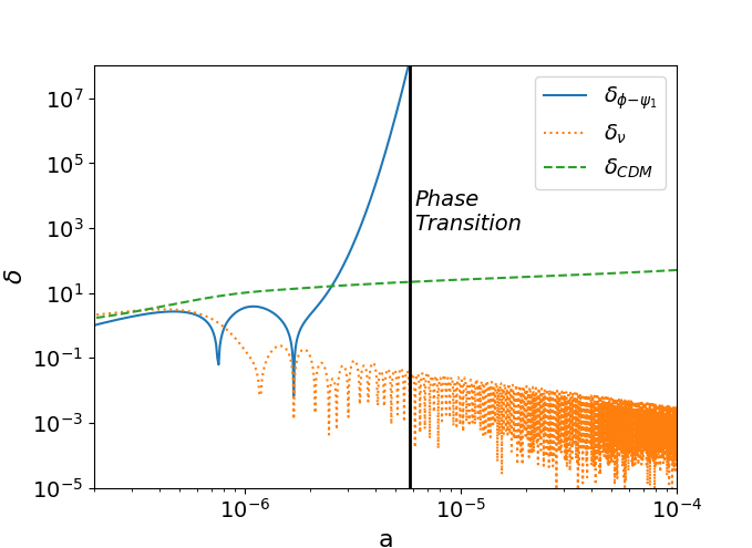
As stated before, the scalar field follows the instantaneous minimum of its potential and this minimum is modulated by the cosmic expansion through the changes in the local neutrino density. So, the mass of the scalar field, can be much larger than the Hubble expansion rate. Consequently, the coherence length of the scalar field, , is much smaller than the present Hubble length. As a consequence of this Afshordi et al. (2005), combined with eq. (8), the sound speed of the neutrino-scalar fluid becomes imaginary once the neutrino becomes non-relativistic followed by instability and formation of nuggets. We have solved the linear perturbation equation (For details see Section 4) to verify this for our choice of quadratic potential. As shown in Fig.1, we compare the evolution of density perturbation of a typical mode (smaller than the range of scalar force) in the radiation dominated era.
3 Solving for the static Profile of the Dark Matter Nugget
The formation of the dense fermionic object in the presence of a scalar mediated force (eg. soliton star, fermionic Q-star) has long been an interesting research topic in different astrophysical contexts (Lee & Pang, 1987; Lynn et al., 1990). The formation of a relativistic star in chameleon theories has also drawn recent interests (Upadhye & Hu, 2009). In the context of neutrino dark energy, formation of neutrino nugget at very late time ( few ) has been studied in Afshordi et al. (2005), while large (Mpc) stable structures of neutrinos clump in the presence of an attractive quintessence scalar has been discussed in Ref. Brouzakis & Tetradis (2006); Brouzakis et al. (2008); Pettorino et al. (2010); Wintergerst et al. (2010). As the quintessence field is extremely light and comparable to Hubble expansion rate (), the range of the fifth force is very large and a neutrino clump can easily be of the order of Mpc size (Casas et al., 2016; Brouzakis et al., 2008). In all of these studies, these Mpc sizes neutrino clumps form at a very late time in cosmic evolution (around few) and thus contribute only a tiny fraction to the dark matter relic density. Whereas we focus on a scalar field with much heavier mass ( eV) and the formation of nuggets takes place at a much earlier redshift (). We show that, as a result, these compact nuggets can, in principle, comprise the entire cold dark matter relic abundance.
In this section we first discuss the qualitative features of the nugget formation, and then numerically solve the bubble profile for the static configuration. For a detailed analysis of the nugget collapse process involving non-linear dynamics, see Narain et al. (2006). We assume that for a critical over density , the sound speed of perturbation becomes negative and the fifth force attracts neutrinos within a Compton sphere of the scalar and finally, Fermi pressure intervenes and balances the attractive scalar force and stable nugget profile is achieved. One can in principle solve the static configuration of nugget by solving coupled Klein-Gordon equation. Taking the metric to have the form
| (11) |
The gravitational mass of the system can be found from asymptotic form of for and is given by Brouzakis & Tetradis (2006)
| (12) |
where, the first term is the gradient energy and the other terms correspond to the dependent fermion mass and the scalar potential .
For our case, the size of the nuggets is very tiny and the scalar force is much stronger than gravity; thus, we can safely ignore gravity and will work with the Minkowski metric.
A general feature of the scalar field static configuration is that the scalar vev changes as a function of distance from the center of the nugget and takes an asymptotic value far away from it. The fermion number density, Fermi pressure are all functions of position through .
As the fermion mass also varies radially, we adopt the Thomas-Fermi approximation as done in Brouzakis & Tetradis (2006) to find the static configuration. In the Thomas-Fermi approximation, one assumes, at each point in space there exists a Fermi sea with local Fermi momentum . With an appropriate scalar potential, it has been shown in Lee & Pang (1987); Lynn et al. (1990) that a degenerate fermionic gas can be trapped in compact objects (even in the absence of gravity) which has been called as soliton star or fermion Q-star. These analyses were done with the zero temperature approximation and in this case, fermions can be modeled as ordinary nuclei. To get an estimate of the nugget radius, we will also work with zero temperature approximation. Soon, we will see that our numerical solution has similarities with these previous works where fermions are extremely light inside the nugget and become increasingly more massive as one moves towards the nugget wall. This ensures positive binding energy and thus the stability of the nuggets.
3.1 Static Solution
Static solutions of this type are mainly governed by two equations. We refer to Brouzakis & Tetradis (2006); Lee & Pang (1987); Chanda & Das (2017) for detailed derivation of these equation. Briefly, the first one is the Klein-Gordon equation for under the potential where the fermions act as a source term for . The other equation tells us how the attractive fifth force is balanced by local Fermi pressure.
As we will be working in the weak field limit of general relativity, the equations can be expressed as
| (13) |
| (14) |
Then, (13) can be rewritten in the simpler following form valid inside the bubble (Brouzakis & Tetradis, 2006),
| (15) |
Outside, there is no pressure, thus this simplifies further
| (16) |
Now with the Thomas Fermi approximation, the distribution function is given by Brouzakis & Tetradis (2006),
| (17) |
With the zero temperature assumption, the distribution function becomes a step function and pressure, energy density and number density take the form:
| (18) |
| (19) |
| (20) |
Thus there are two unknown quantities, namely and , whose values are determined by solving the two coupled equations (14) and (15). Evaluating the integrations in eq. (18)-(20), we find an explicit form for the trace of energy-momentum tensor, :
| (21) |
Furthermore the pressure is found to be of the form
| (22) |
where .


3.2 Initial conditions and model parameters
Using eqs. (22) and (21) in eq. (14), we obtain an equation for the local Fermi momentum which needs to be solved with proper boundary conditions. This initial condition is chosen appropriately to match the total number of fermions initially within a Compton volume of the scalar before the onset of instability. First, we solve for and using that we numerically solve the Klein-Gordon equation (5) to obtain the profile.
The Klein-Gordon equation closely resembles the dynamics of a particle moving under a Newtonian potential when “” is replaced by time “” and “” is replaced by the position of the particle. The static solution corresponds to a final particle position which is asymptotically at rest. This is only possible for a particular set of initial condition and For the solution to be well behaved at the center of the nugget, should not have a term like which demands . The other initial condition is obtained by numerical iteration i.e. by identifying a particular for which the numerical solution gives , where is the cosmological value outside the nugget. For our case, which is the minima of the potential. Once we find and , it is straightforward to obtain the fermion mass and fermion number density as a function of distance from the center of the nugget. The radius of the nugget is determined when the number density drops to zero.
Next, we numerically find the static profiles for the scalar field for two toy examples to show that indeed stable nugget can be formed.
3.2.1 Example 1
We first consider fermions of mass which are trapped in nuggets and using, , so to obtain an example static profile for . The Fermi momentum is fixed by identifying a value for which , one solution is:
| (23) |
The inferred is then used on the energy-momentum tensor to solve eq. (13). We take with the external potential and the resulting static profile of the scalar field (as shown in Fig.2), is obtained from the boundary condition
| (24) |
and we evaluate the profile for .
The mass variation of trapped fermion inside the nugget is depicted as in Fig.3. The total nugget mass is found to be , which with the chosen scalar field mass, corresponds to a dark matter relic density at the nugget formation of order .
3.2.2 Example 2
We repeat the same treatment with a different choice for the Fermi momentum boundary value
| (25) |
and boundary condition for the solution
| (26) |
so to obtain an static profile for ., with and . This parameter set suggests a total nugget mass and a dark matter relic density of at the time of nugget formation.
3.3 Possibility of a homogeneous marginally stable tenuous phase of neutrino gas?
Now we would like to explain an important issue regarding our zero temperature approximation of nugget formation. Here we discuss whether our assumption of forming cold nuggets surrounded by vacuum as a result of phase transition is realistic or not. Because another possible outcome can be formation of dense nuggets, surrounded by a tenuous hot gas of neutrinos. But it seems like instability in mass varying neutrino prefers the former! The explanation for this can be obtained by following the discussion in the paper Afshordi et al. (2005) where a detailed instability study in ”mass varying of neutrino dark energy” was first carried out. They showed that the density of neutrinos in the tenuous gas phase (which is not trapped in nugget) is exponentially suppressed and that the most probable outcome of the instability is the formation of dense nuggets surrounded by practically empty space without any marginally stable tenuous gas of neutrino interacting with scalar. The main reason they found why we don’t see a tenuous gas phase in this phase transition is mainly for two reasons . First of all, the time scale of instability is much smaller than Hubble time scale unlike the standard quintessence model of dark energy . As mass of the scalar field here is much higher than Hubble parameter during MRE, one can assume a very rapid formation of nugget compared to cosmological Hubble time scale. They showed that the imaginary speed of sound is indeed scale-independent in any non-relativistic MaVaNs models, making the instability most severe at the microscopic scales (). The fraction of neutrinos in the gas phase is computed by the equilibrium of evaporation rate from and accretion rate onto the surface of the nuggets. However, the large density contrast between inside and outside of the nuggets implies that only neutrinos with a large Lorentz factor can escape the nuggets. This is also obvious from our plot of variation of neutrino mass as function of distance from nugget center. So with the above arguments we believe our zero temperature assumption will be the most probable scenario of such phase transition but of course non-linearity can bring surprise and is kept for future research.
4 Cosmology of phase transition
Dark Matter nugget formation from instability in neutrino is a unique phenomenon and it may have some interesting effect on both CMB and linear structure formation. In this section, we explore these effects if we let this phenomenon to account for the entire DM density in the universe. To find the effect of the nugget formation in CMB and linear structure formation, we need to solve for the linear as well as perturbation equations for the whole cosmic history. We adopt the generalized dark matter(GDM) formalism describe our interacting - fluid. In this formalism, the background equation of the fluid is parameterized by its equation of state, which we take to be a function of the redshift . At early times, since we assume the fluid to be relativistic, the coupling between neutrino and the scalar field can be ignored. So, we take at high redshifts. Then, as the neutrinos become non-relativistic around a critical redshift , an EDE like phase appears when the scalar field relaxes into the effective minima followed by an intermediate transition period where the effective equation of state goes below zero to . During this period, sound speed square, also becomes negative and we have instability in the fluid. Immediately after that, phase transition happens as a result of the instability and the fluid transitions into DM nugget state, where .
The perturbations equations for our fluid in synchronous gauge from the GDM formalism are given by:
| (27) | |||||
| (28) |
To solve the background and the perturbation equations, we modify the CLASS Boltzmann code (Blas et al., 2011) to replace the CDM component with an extra fluid component which describes our fluid through and . In Fig.1, we indeed see that around , the density fluctuations of the - fluid shoots up to a huge value compared to those of the other components such CDM and neutrinos from standard CDM scenario. In Fig. 3(right), we plot the fractional energy density of the dominant components of the universe at different times against redshift for the case . We see that in early times, radiation is the dominant component as usual but a tiny yet significant portion of the universe () consists of - as dark radiation. Then around , - transitions from radiation into matter like state and starts to fall while rises. The Matter-radiation equality happens at . The DM nugget energy density dominates the universe until crosses at late times (). The value of today comes out to be which is equal to the dark matter density today according to CDM.
In Fig.3(left), we plot the CMB temperature anisotropy spectrum along with the residuals from Planck CDM data Ade et al. (2016) for three different critical redshifts, . We see that the later the critical redshift is, the more it deviates from CDM . For the case , the residuals go beyond the error bar set by Planck. The residual plot is also dependent on the extent of the transition period which we haven’t considered in this paper. A proper MCMC analysis is needed to find a suitable and the extent of the transition period which is left for future work.

4.1 DM density and
One can easily estimate dark matter density as nuggets are highly non-relativistic and assuming one nugget forming in each Compton volume of the scalar , the energy density of dark matter at the formation redshift is simply given by
| (29) |
Evolving this to today implies
where is the nugget mass. We mainly focus on the case when nuggets form only a sub-fraction of DM and most of the energy density of EDE phase goes into scalar dynamics.
At early time before neutrino turns semi-relativistic and starts to couple to scalar field, the neutrino-scalar fluid was behaving like dark radiation. But during CMB this fluid does not does not behave as radiation as phase transition has already changed its equation of state during MRE. But never the less very small scale modes which was inside the horizon at very early epoch would be slightly affected and have tiny imprint on CMB too. To see this effect, we numerically solve and plot the CMB power spectra deviation in Fig. 3 and we see that a redshift of transition is within the error bar of Planck.
Also, in our MCMC analysis in next section, we will see that statistically our model performs quite well when confronted with Planck, local and BAO data sets.
Never the less, if one is interested in very early epoch and especially epoch of BBN, the amount of dark radiation in our model is estimated Das & Nadler (2020)
| (30) |
This excess radiation is well with in the BBN bound. The matter power spectra form this late dark matter neutrino nuggets has sharp cut-off in small scales which has lot of interesting small scale effects and has recently been studied in Das & Nadler (2020).
4.2 Nugget life time and production of scalar radiation
In our model, after its formation, nuggets can produce scalar dark radiation through two body annihilation of sterile neutrino like particle in the dense environment inside the nugget. In this section, we show that the nuggets are stable enough to be dark matter by calculating the annihilation rate of into inside the nugget. As the scalar is much lighter ( eV) than fermion, we are interested in the annihilation process: .
From our numerical results, it is clear that fermion mass is extremely light closer to the center of the nugget and becomes heavier at the wall. For the same reason, integrating out heavy field is a valid approximation inside the nugget (numerically verified) and the fermion mass term is given by . Inside the nugget, the coupling constant , between light fermion and is defined through the following interaction term
| (31) |
where is fluctuation in the field.
We find that , the value of the coupling inside the nugget, is very tiny: . The nugget lifetime can be estimated for a given . In terms of the number density of the fermion inside the nugget(), the annihilation rate is given by
| (32) |
where is the center of mass energy. Integrating, we can estimate the half life of the nugget
| (33) |
where is the volume of the nugget and is the central number density at . Taking the specific example of a dark matter nugget studied in the previous example, and substituting the values from this numerical solution, we find half life of the nugget is roughly s. This is much larger than the age of the universe sec.
5 Hubble anomaly in connection to our model
In this section, we discuss the recent Hubble anomaly in the context of our model mainly for two reasons.
The first reason is- before the nugget formation, the neutrino-scalar fluid naturally goes through short early dark energy domination as explained before. Given that the early DE model has been proposed as one most prominent solution of Hubble anomaly, we explore if our model can be realized as a successful candidate for EDE scenario arising from (sterile) neutrino-scalar interaction.
The second reason is, in a generic EDE model, from the theoretical perspective, the physics of matter-radiation equality and early dark energy are completely disconnected - which requires fine-tuning in order for them to appear nearly simultaneously. Our model is based on physics where scalar mass is of the order of neutrino mass scale (unlike in Sakstein & Trodden (2020), where scalar mass is tuned to an extraordinarily small value, like in the case of quintessence theories) as proposed originally in the theories of neutrino dark energy and the similarity of neutrino mass and MRE scale naturally gives early dark energy phase prior to MRE. In a neutrino-scalar interaction scenario, the background equation for the neutrinos is given by
| (34) |
where the right-hand side is the interaction term. We see that when neutrinos are relativistic, the interaction term is negligible since . Therefore, the interaction is only prominent when the neutrinos become non-relativistic around and its equation of state drops below ( the exact value depends on the potential) and the fluid starts to behave like dark energy. This early phase of DE is only active for a short duration(see right panel of Fig. 9) followed by its disappearance as nugget formation takes place. The excess dark energy gives a local boost to local Hubble expansion rate and the sound horizon for acoustic waves in the photon-baryon fluid, is given by
| (35) |
Since H(z) in the EDE scenario was higher than that of CDM for a short period of time, it would mean that is reduced compared to the CDM model. The angular diameter distance to the last scattering surface is given by
| (36) |
where is the angular scale of the sound horizon at matter-radiation equality. This angular scale is fixed as it is solely determined by CMB observation and hence its value is not sensitive to any model. This implies that also gets reduced in this scenario. Since is inversely proportional to the Hubble constant, this means is higher than it is in CDM.

5.1 Simple model (A): Neutrino EDE entirely transitions to CDM
First we consider the most simple case when
the entire energy of the EDE phase goes into the dark matter state. This is assuming all the neutrinos clumps inside the nugget and the scalar field after being released coherently oscillates around quadratic potential which also behaves like dark matter provided it does not decay into other lighter particles Bjaelde & Das (2010). The evolution of equation of state of the scalar fluid is shown in right panel of Fig. 9 where in most of the radiation dominated era ( except when neutrino turns non-relativistic) the neutrino-scalar fluid behaves like radiation with followed by a dark energy like behavior ( the exact value depends on potential and finally after nugget formation the equation of state becomes likex CDM .
We numerically find that this case cannot (or only partially) resolve the Hubble anomaly. This is expected as from original EDE study Poulin et al. (2019) where it is shown that the early dark energy phase should dilute at least like radiation or faster to resolve Hubble anomaly completely. However, now we discuss that in extended models of our scenario, it is highly possible that a major fraction of early DE phase indeed goes into the scalar field which redshifts much faster than radiation. This is realised when the quadratic potential is slightly modified at and the scalar field redshifts away its initial energy through a kinetic energy dominated phase, similar to Alexander & McDonough (2019); Lin et al. (2019).


5.2 Extended model (B): Neutrino EDE dilutes as Kinetic energy dominated phase Kination
5.2.1 Evolution of scalar immediately after nugget formation
As discussed before, most probable outcome of the instability is the formation of dense non-linear structures of nuggets, surrounded by practically empty space where the scalar starts to role toward its true minima as the effective minima disappears in a time scale which is much smaller than the local Hubble time. Thus the dynamics of the fluid is indeed dominated by a kinetic energy phase and EDE energy dilutes much faster than radiation.
After the nugget formations, neutrinos in the “gas phase ( a tiny fraction of total neutrino)” continuously lose energy to Hubble expansion, and nuggets, due to their small volume fraction, cannot significantly affect the gas phase. As a result most of the neutrinos should accrete into the nuggets. In fact, in Sec. V of Afshordi et al. (2005) they showed that within the assumption of
thermal equilibrium, this process instantly exhausts the
neutrinos outside the nuggets and scalar field settles at its true vacuum within the gas phase.
In the conventional quintessence models, similar to inflationary models, the scalar field is slowly rolling, and therefore its effective mass is smaller than the Hubble expansion rate. In contrast, in mass varying dark energy model, the scalar field sits at the instantaneous minimum of its potential, and the cosmic expansion only modulates this minimum through changes in the local neutrino density. So once the nugget forms surrounded by practically empty space, the scalar field quickly settles to its true minima globally. As a result our kination picture is the most natural outcome of this scenario.
So as stated before, unlike the general EDE model, our early dark energy phase is not controlled by local Hubble friction rather neutrino density. But after the nugget formation, scalar decouples from neutrino density and its evolution is determined by Klein Gordon equation
| (37) |
It is instructive to note that here we have neglected the term. In our case, though scalar field profile varies around nuggets, we realise that nugget size ( as seen from Fig.2 ) is much smaller than the Compton length of the scalar field. As can be seen from the same figure - the scalar field value varies within a length scale cm where the the Compton length of the scalar cm. ( this corresponds to our scalar mass in the first numerical example). So within our assumption, the scalar field would sense the nuggets as point objects ( as the spatial variation scale of is times smaller than scalar Compton length). On top, the number density of such point like nugget within one Compton volume is extremely low– more or less one nugget within each Compton volume of scalar. This also justifies our assumption. Our situation is similar to chameleon theory Khoury & Weltman (2004) where in small distance (solar to galactic scale) chameleon scalar spatial variation is non-negligible but in cosmological distance ( ) the field is controlled by Klein Gordon equation without a term. But in our scenario, if nuggets merge and continuous merger make the final nugget radius comparable to scalar Compton length, the contribution might be important. This will be clear when we study nugget collision and change of scalar profile due to merger. This is beyond the scope of present work and has been kept for future research. Specially, if larger sterile neutrino halo forms due to merger as well as virialisation, one needs to incorporate contribution to K.G. equation and it would be interesting to see how it changes scalar field dynamics. It is also important to note that the initial condition for our case when the field starts to be dynamical would be very different than Poulin et al. (2019) where field starts to roll of when mass of the field becomes larger than Hubble friction. Moreover, it is possible to have a steeper potential where the scalar field is held in the effective minima and rolls off very fast (dominated by kinetic energy (Alexander & McDonough, 2019; Braglia et al., 2020)) as soon as the field is released during the onset of nugget formation. In this scenario it is shown that the EDE rapidly redshifts away and thus solving the Hubble anomaly.
5.2.2 Choice of potential
We have pointed out earlier that a quadratic potential is most natural in mass varying neutrino DE in the particle physics context of re-normalization. On the other hand, a quadratic potential was recently used in the Acoustic Dark Energy (ADE) model of Lin et al. (2019) where for and for . Here, the whole potential energy converts into kinetic energy and hence . is cut off for negative values of such that there is no oscillation and no kinetic energy can convert back into potential energy. Another potential where it is possible realize similar scenario by taking a potential which is within the frame work of -attractor potential where inflationary potential is unified with late DE like behavior. In the case ”C” of Braglia et al. (2020), they take a potential . This potential is flat enough(see Fig.1 of Braglia et al. (2020)) so that the scalar field does not oscillate around the minimum after rolling off and instead, it remains in kination until its fractional energy density becomes insignificant and then freezes out after exhausting all its inertia.

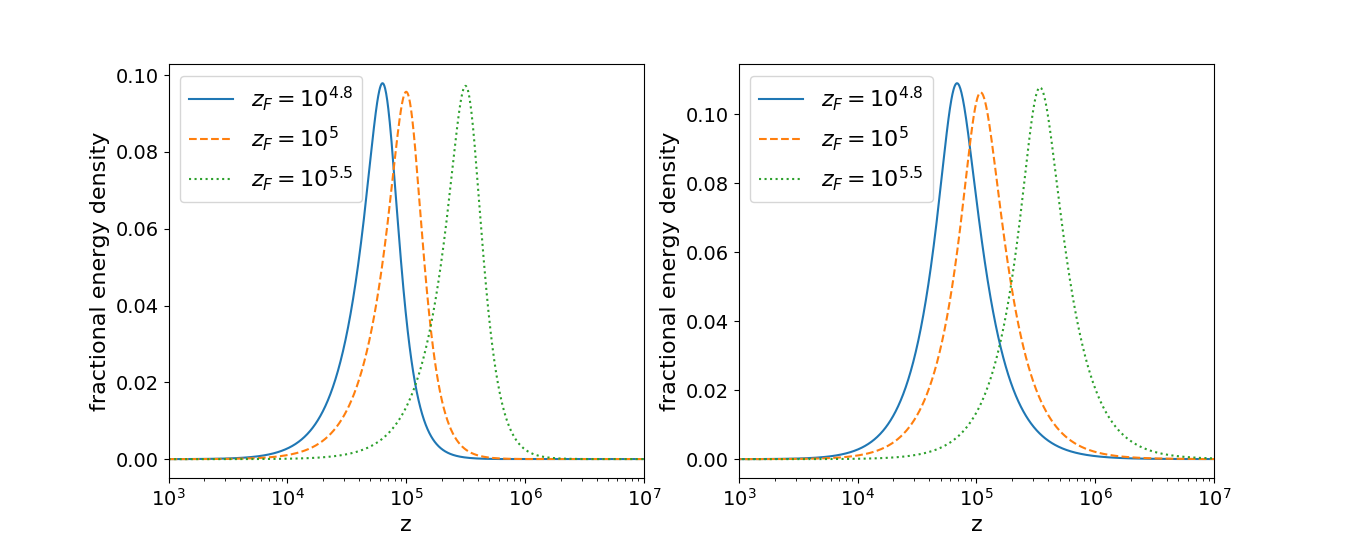
In Fig. 9, we plot the fractional energy density of the fluid against redshift for three different for the cases where w rises from to 1 (left panel) and from (right panel) to 1 after decoupling around . It is shown in Karwal & Kamionkowski (2016); Hill et al. (2020) that around 5 to 10 percent rise in fractional energy of EDE followed by a quick decay is required to resolve Hubble anomaly. We see a similar behaviour in our numerical solution Fig. 9.
6 MCMC Analysis
Here we do a simplest case MCMC analysis for a neutrino scalar fluid with a quadratic potential. We assume after the phase transition, the kination period dominates and most of the energy of neutrino-EDE dilutes fast as . Our MCMC analysis indeed shows that this phase transition indeed relaxes the Hubble anomaly.
6.1 Details Of Analysis
To perform Monte Carlo Markov Chain (MCMC) analysis, we will be using CMB/BAO data sets along with SH0ES prior.The Details of our data set are following:
-
•
Planck 2018 measurements of the low- CMB TT, EE, and high- TT, TE, EE power spectra, together with the gravitational lensing potential reconstruction (Aghanim et al., 2018).
- •
-
•
The measurements of the growth function (FS) from the CMASS and LOWZ galaxy samples of BOSS DR12 at , , and (Alam et al., 2017).
-
•
The Pantheon SNIa catalogue, spanning redshifts (Scolnic et al., 2018).
-
•
The SH0ES result, modelled with a Gaussian likelihood centered on km/s/Mpc (Riess et al., 2019); however, choosing a different value that combines various direct measurements would not affect the result, given their small differences.
To better understand the extent to which the model can resolve the tension, we perform analysis with the SH0ES prior as done for most of EDE models in the literature. Our baseline cosmology consists in the following combination of the six CDM parameters , plus two extra parameters of EDE , namely . We dub this model as EDE. We confront the CDM model with SH0ES prior and run our MCMCs with the Metropolis-Hasting algorithm as implemented in the MontePython-v3 (Thejs Brinckmann, 2018) code interfaced with our modified version of CLASS. All reported are obtained with the python package iMinuit 111https://iminuit.readthedocs.io/ (James & Roos, 1975). We make use of a Choleski decomposition to better handle the large number of nuisance parameters (Lewis et al., 2000) and consider chains to be converged with the Gelman-Rubin convergence criterium (Gelman & Rubin, 1992).
6.2 Results of MCMC Analysis
The parameter constraints obtained from EDE and CDM using Planck+Ext+SH0ES data are shown in table 1. Where ’Ext’ represents combined ’’. We also have reported for each model in table 1.
The 2d posterior distributions for EDE along with CDM and acoutic dark energy (ADE) model are shown in figure 10 .
From the results, we have evidence for non-zero at a epoch of transition . To be precise we have got bestfit of =0.05631 and redshift =1903.7 resulting a significantly higher value of Hubble parameter .
With this value of Hubble parameter, we are in agreement of nearly 1.3 with SH0ES measurement which is km/s/Mpc (Riess et al., 2019). For better visualization please refer to the figure 10, where we have shown 1(dark green) and 2(light green) bands of SH0ES measurements of Hubble parameter. In terms of the goodness of fit, numbers that we have shown in table 1. We got an improvement of =-10.51 which shows the Planck+Ext+SH0ES data prefers EDE cosmology over CDM cosmology.
If we compare Our results of EDE cosmology with Accoustic Dark Energy(ADE) cosmology (Lin et al., 2019), our EDE cosmology is doing marginally better in terms of agreement with SH0ES measurement and measurements of the amplitude of local structure. As we can see we get a smaller than ADE models. Detailed Analysis will be done separately in near future using a different cosmological tool (D’Amico et al., 2020) and it is beyond the scope of this paper.
| Model | CDM | Early mass varying neutrino DE |
|---|---|---|
| Parameter | Planck+Ext+SH0ES | Planck+Ext+SH0ES |
| 2 | ||
| [km/s/Mpc] | ||
| (CDM) | 0 | -10.51 |

But unlike other EDE model, our DE scale is not fine tuned rather EDE emerges naturally during MRE because of similarity of light sterile neutrino mass and Temperature of Universe at around matter radiation equality. So our model is a non-fine tuned EDE model which also statistically preferred over LCDM and resembles EDE or acoustic DE models. As, building a viable EDE model without fine-tuning of dark energy scale is very difficult, we feel, our neutrino mass driven EDE is a step forward for a successful non- fine tuned model of early dark energy and it’s worth exploring in details as future research. It is true that like other EDE or Acoustic DE model, our models is also challenged by LSS data as shown in Hill et al. (2020) . But our value is slightly smaller than standard ADE models. On top there are two points we would like to mention.
-
•
Recently, after Hill et al. (2020), there has been another work Smith et al. (2020b) where they have shown that EDE models are constrained but not ruled out by LSS data-specially galaxy power spectrum measuremnt aspect of LSS is fine with EDE models while recent weak lensing KiDS/Viking Joudaki et al. (2020); Hildebrandt et al. (2020) put strong constraints on it. So, EDE models are still an active area of research and we feel near future LSS data will determine its fate. But as seen from initial MCMC run, our model somehow does not make worse like EDE or ADE models as seen in figure 10.
-
•
On top, our model has an extra feature which we guess, will help us when confronted with LSS data in future. The nuggets can evaporate in scalar radiation as mentioned in Afshordi et al. (2005). That will make the gravitational potential decay and suppress the matter power spectra and might alleviate LSS difficulty completely. It was shown in Pandey et al. (2020) that even 1 or 2 % of DM decays into radiation after decoupling, it can alleviate tension significantly. How much radiation the nuggets produce and depending on whether they are thermal or non-thermal bath, it will modify our matter power spectra. This needs detailed analysis and we hope to report this aspect in near future.
7 Conclusion
Data from MiniBooNE experiment might indicate the existence of light sterile neutrino states of mass (sub-eV to 10 eV). Though this lighter sterile neutrino has relevant properties, in general, light eV-mass sterile fermions are not viable cold dark matter (CDM) candidate due to its excessive free-streaming. Here in this paper
-
•
We realize a scenario of nugget formation with sterile neutrino in radiation dominated era close to MRE. We analytically show that the condition of instability is generic even with quadratic potential in RDE when sterile neutrino turns non-relativistic followed by nugget formation. Our scenario provides a complete new way of producing a cold dark matter nuggets from light eV sterile neutrino. This dark matter can contribute to a considerable fraction of DM density today depending on model paramters.
-
•
Using Thomas Fermi approximation and solving coupled Klein Gordon equation numerically, we find the static configuration of the scalar field which allows us to calculate nugget mass, radius of nugget and dark matter density. The detailed nugget profile was never solved before in neutrino DE model. The mass of the nugget in our two examples are eV and eV and the corresponding redshift of nugget formation are and respectively. For these formation redshifts , we show that the entire dark matter density of the university can arise from this heavy neutrino nuggets!
-
•
We use quadratic scalar potential for the scalar field as it keeps the radiative correction to the potential under control as illustrated in super-symmetric theories of neutrino dark energy (Fardon et al., 2006). Also we use most general Yukawa type coupling in dark sector as proposed in original neutrino dark energy model.
-
•
This natural phase transition prior to MRE in Early neutrino dark energy has strong implications for recent Hubble tension. This model of EDE does not require a fine-tuned dark energy scale yet it can comprise around 10 percent of total energy budget around MRE ( as needed to solve Hubble anomaly (Poulin et al., 2016, 2019)). This early dark energy decays faster than radiation as the nugget forms and scalar rolls of freely along the quadratic potential dominated by a kinetic energy phase. In our case, the DE energy injection and its decay ( due to phase transition) is entirely controlled by sterile neutrino mass and in principle our scenario can realise a viable early DE particle physics model which can solve Hubble tension. EDE models are still an active area of research and we feel near future LSS data will determine its fate. But as seen from initial MCMC run, our model is consistent with higher and does not make worse like EDE or ADE models as seen in figure 10. A detailed LSS data analysis is required to precisely tell how well our model performs and what kind of potential of scalar field is preferred when confronted with large scale structure data from galaxy survey or recent weak lensing measurements. This will be reported in near future.
Acknowledgements
We thank Vivian Poulin and Ethan Nadler for giving us comments on the draft. We also thank Marc Kamionkowski for suggesting us to adopt generalized dark matter formalism for neutrino-scalar fluid and look for instability in terms of sound speed. We are grateful to James Unwin for reading the manuscript and giving us valuable suggestions. We thank Neal Weiner and Kris Sigurdson for helpful discussions during the initial phase of the work. SD thanks IUSSTF-JC-009-2016 award from the Indo-US Science & Technology Forum which supported the project.
References
- Abazajian (2006) Abazajian, K. 2006, Phys. Rev. D, 73, 063513, doi: 10.1103/PhysRevD.73.063513
- Abazajian & Kusenko (2019) Abazajian, K. N., & Kusenko, A. 2019, Phys. Rev. D, 100, 103513, doi: 10.1103/PhysRevD.100.103513
- Acero & Lesgourgues (2009) Acero, M. A., & Lesgourgues, J. 2009, Phys. Rev. D, 79, 045026, doi: 10.1103/PhysRevD.79.045026
- Ade et al. (2016) Ade, P., et al. 2016, Astron. Astrophys., 594, A13, doi: 10.1051/0004-6361/201525830
- Afshordi et al. (2005) Afshordi, N., Zaldarriaga, M., & Kohri, K. 2005, Phys. Rev. D, 72, 065024, doi: 10.1103/PhysRevD.72.065024
- Aghanim et al. (2018) Aghanim, N., et al. 2018. https://arxiv.org/abs/1807.06209
- Agrawal et al. (2019) Agrawal, P., Cyr-Racine, F.-Y., Pinner, D., & Randall, L. 2019. https://arxiv.org/abs/1904.01016
- Aguilar-Arevalo et al. (2010) Aguilar-Arevalo, A., et al. 2010, Phys. Rev. Lett., 105, 181801, doi: 10.1103/PhysRevLett.105.181801
- Aguilar-Arevalo et al. (2013) —. 2013, Phys. Rev. Lett., 110, 161801, doi: 10.1103/PhysRevLett.110.161801
- Aguilar-Arevalo et al. (2018) —. 2018, Phys. Rev. Lett., 121, 221801, doi: 10.1103/PhysRevLett.121.221801
- Alam et al. (2017) Alam, S., et al. 2017, Mon. Not. Roy. Astron. Soc., 470, 2617, doi: 10.1093/mnras/stx721
- Alexander & McDonough (2019) Alexander, S., & McDonough, E. 2019, Phys. Lett. B, 797, 134830, doi: 10.1016/j.physletb.2019.134830
- Bell et al. (2006) Bell, N. F., Pierpaoli, E., & Sigurdson, K. 2006, Phys. Rev. D, 73, 063523, doi: 10.1103/PhysRevD.73.063523
- Beutler et al. (2011) Beutler, F., Blake, C., Colless, M., et al. 2011, Mon. Not. Roy. Astron. Soc., 416, 3017, doi: 10.1111/j.1365-2966.2011.19250.x
- Bezrukov et al. (2010) Bezrukov, F., Hettmansperger, H., & Lindner, M. 2010, Phys. Rev. D, 81, 085032, doi: 10.1103/PhysRevD.81.085032
- Bjaelde & Das (2010) Bjaelde, O. E., & Das, S. 2010, Phys. Rev. D, 82, 043504, doi: 10.1103/PhysRevD.82.043504
- Blas et al. (2011) Blas, D., Lesgourgues, J., & Tram, T. 2011, JCAP, 07, 034, doi: 10.1088/1475-7516/2011/07/034
- Blinov & Marques-Tavares (2020) Blinov, N., & Marques-Tavares, G. 2020. https://arxiv.org/abs/2003.08387
- Blomqvist et al. (2019) Blomqvist, M., et al. 2019, Astron. Astrophys., 629, A86, doi: 10.1051/0004-6361/201935641
- Boyarsky et al. (2009) Boyarsky, A., Lesgourgues, J., Ruchayskiy, O., & Viel, M. 2009, Phys. Rev. Lett., 102, 201304, doi: 10.1103/PhysRevLett.102.201304
- Braglia et al. (2020) Braglia, M., Emond, W. T., Finelli, F., Gumrukcuoglu, A. E., & Koyama, K. 2020. https://arxiv.org/abs/2005.14053
- Brouzakis & Tetradis (2006) Brouzakis, N., & Tetradis, N. 2006, JCAP, 01, 004, doi: 10.1088/1475-7516/2006/01/004
- Brouzakis et al. (2008) Brouzakis, N., Tetradis, N., & Wetterich, C. 2008, Phys. Lett. B, 665, 131, doi: 10.1016/j.physletb.2008.05.068
- Casas et al. (2016) Casas, S., Pettorino, V., & Wetterich, C. 2016, Phys. Rev. D, 94, 103518, doi: 10.1103/PhysRevD.94.103518
- Chanda & Das (2017) Chanda, P. K., & Das, S. 2017, Phys. Rev. D, 95, 083008, doi: 10.1103/PhysRevD.95.083008
- Chudaykin et al. (2020) Chudaykin, A., Gorbunov, D., & Nedelko, N. 2020, JCAP, 08, 013, doi: 10.1088/1475-7516/2020/08/013
- D’Amico et al. (2020) D’Amico, G., Senatore, L., & Zhang, P. 2020. https://arxiv.org/abs/2003.07956
- Das et al. (2006) Das, S., Corasaniti, P. S., & Khoury, J. 2006, Phys. Rev. D, 73, 083509, doi: 10.1103/PhysRevD.73.083509
- Das & Nadler (2020) Das, S., & Nadler, E. O. 2020. https://arxiv.org/abs/2010.01137
- Das & Weiner (2011) Das, S., & Weiner, N. 2011, Phys. Rev. D, 84, 123511, doi: 10.1103/PhysRevD.84.123511
- Dasgupta & Kopp (2014) Dasgupta, B., & Kopp, J. 2014, Phys. Rev. Lett., 112, 031803, doi: 10.1103/PhysRevLett.112.031803
- de Sainte Agathe et al. (2019) de Sainte Agathe, V., et al. 2019, Astron. Astrophys., 629, A85, doi: 10.1051/0004-6361/201935638
- Dodelson & Widrow (1994) Dodelson, S., & Widrow, L. M. 1994, Phys. Rev. Lett., 72, 17, doi: 10.1103/PhysRevLett.72.17
- Fardon et al. (2004) Fardon, R., Nelson, A. E., & Weiner, N. 2004, JCAP, 10, 005, doi: 10.1088/1475-7516/2004/10/005
- Fardon et al. (2006) —. 2006, JHEP, 03, 042, doi: 10.1088/1126-6708/2006/03/042
- Gell-Mann et al. (1979) Gell-Mann, M., Ramond, P., & Slansky, R. 1979, Conf. Proc. C, 790927, 315. https://arxiv.org/abs/1306.4669
- Gelman & Rubin (1992) Gelman, A., & Rubin, D. B. 1992, Statist. Sci., 7, 457, doi: 10.1214/ss/1177011136
- Gilman et al. (2020) Gilman, D., Birrer, S., Nierenberg, A., et al. 2020, Mon. Not. Roy. Astron. Soc., 491, 6077, doi: 10.1093/mnras/stz3480
- Hannestad et al. (2010) Hannestad, S., Mirizzi, A., Raffelt, G. G., & Wong, Y. Y. 2010, JCAP, 08, 001, doi: 10.1088/1475-7516/2010/08/001
- Hildebrandt et al. (2020) Hildebrandt, H., et al. 2020, Astron. Astrophys., 633, A69, doi: 10.1051/0004-6361/201834878
- Hill & Baxter (2018) Hill, J. C., & Baxter, E. J. 2018, JCAP, 08, 037, doi: 10.1088/1475-7516/2018/08/037
- Hill et al. (2020) Hill, J. C., McDonough, E., Toomey, M. W., & Alexander, S. 2020, Phys. Rev. D, 102, 043507, doi: 10.1103/PhysRevD.102.043507
- Humphreys et al. (2013) Humphreys, E., Reid, M. J., Moran, J. M., Greenhill, L. J., & Argon, A. L. 2013, Astrophys. J., 775, 13, doi: 10.1088/0004-637X/775/1/13
- Ichikawa et al. (2007) Ichikawa, K., Kawasaki, M., Nakayama, K., Senami, M., & Takahashi, F. 2007, JCAP, 05, 008, doi: 10.1088/1475-7516/2007/05/008
- Irˇsič et al. (2017) Irˇsič, V., et al. 2017, Phys. Rev. D, 96, 023522, doi: 10.1103/PhysRevD.96.023522
- Ivanov et al. (2020) Ivanov, M. M., McDonough, E., Hill, J. C., et al. 2020. https://arxiv.org/abs/2006.11235
- James & Roos (1975) James, F., & Roos, M. 1975, Computer Physics Communications, 10, 343, doi: 10.1016/0010-4655(75)90039-9
- Jedamzik et al. (2020) Jedamzik, K., Pogosian, L., & Zhao, G.-B. 2020. https://arxiv.org/abs/2010.04158
- Joudaki et al. (2020) Joudaki, S., et al. 2020, Astron. Astrophys., 638, L1, doi: 10.1051/0004-6361/201936154
- Karwal & Kamionkowski (2016) Karwal, T., & Kamionkowski, M. 2016, Phys. Rev. D, 94, 103523, doi: 10.1103/PhysRevD.94.103523
- Khoury & Weltman (2004) Khoury, J., & Weltman, A. 2004, Phys. Rev. Lett., 93, 171104, doi: 10.1103/PhysRevLett.93.171104
- Kodama & Sasaki (1984) Kodama, H., & Sasaki, M. 1984, Prog. Theor. Phys. Suppl., 78, 1, doi: 10.1143/PTPS.78.1
- Laine & Shaposhnikov (2008) Laine, M., & Shaposhnikov, M. 2008, JCAP, 06, 031, doi: 10.1088/1475-7516/2008/06/031
- Lee & Pang (1987) Lee, T., & Pang, Y. 1987, Phys. Rev. D, 35, 3678, doi: 10.1103/PhysRevD.35.3678
- Lewis et al. (2000) Lewis, A., Challinor, A., & Lasenby, A. 2000, ApJ, 538, 473, doi: 10.1086/309179
- Lin et al. (2019) Lin, M.-X., Benevento, G., Hu, W., & Raveri, M. 2019, Phys. Rev. D, 100, 063542, doi: 10.1103/PhysRevD.100.063542
- Lynn et al. (1990) Lynn, B. W., Nelson, A. E., & Tetradis, N. 1990, Nucl. Phys. B, 345, 186, doi: 10.1016/0550-3213(90)90614-J
- Mohapatra & Senjanovic (1980) Mohapatra, R. N., & Senjanovic, G. 1980, Phys. Rev. Lett., 44, 912, doi: 10.1103/PhysRevLett.44.912
- Nadler et al. (2020) Nadler, E., et al. 2020. https://arxiv.org/abs/2008.00022
- Narain et al. (2006) Narain, G., Schaffner-Bielich, J., & Mishustin, I. N. 2006, Phys. Rev. D, 74, 063003, doi: 10.1103/PhysRevD.74.063003
- Niedermann & Sloth (2019) Niedermann, F., & Sloth, M. S. 2019. https://arxiv.org/abs/1910.10739
- Niedermann & Sloth (2020a) —. 2020a. https://arxiv.org/abs/2006.06686
- Niedermann & Sloth (2020b) —. 2020b. https://arxiv.org/abs/2009.00006
- Pandey et al. (2020) Pandey, K. L., Karwal, T., & Das, S. 2020, JCAP, 07, 026, doi: 10.1088/1475-7516/2020/07/026
- Petraki & Kusenko (2008) Petraki, K., & Kusenko, A. 2008, Phys. Rev. D, 77, 065014, doi: 10.1103/PhysRevD.77.065014
- Pettorino et al. (2010) Pettorino, V., Wintergerst, N., Amendola, L., & Wetterich, C. 2010, Phys. Rev. D, 82, 123001, doi: 10.1103/PhysRevD.82.123001
- Poulin et al. (2016) Poulin, V., Serpico, P. D., & Lesgourgues, J. 2016, JCAP, 08, 036, doi: 10.1088/1475-7516/2016/08/036
- Poulin et al. (2018) Poulin, V., Smith, T. L., Grin, D., Karwal, T., & Kamionkowski, M. 2018, Phys. Rev. D, 98, 083525, doi: 10.1103/PhysRevD.98.083525
- Poulin et al. (2019) Poulin, V., Smith, T. L., Karwal, T., & Kamionkowski, M. 2019, Phys. Rev. Lett., 122, 221301, doi: 10.1103/PhysRevLett.122.221301
- Riess et al. (2019) Riess, A. G., Casertano, S., Yuan, W., Macri, L. M., & Scolnic, D. 2019, Astrophys. J., 876, 85, doi: 10.3847/1538-4357/ab1422
- Riess et al. (2016) Riess, A. G., et al. 2016, Astrophys. J., 826, 56, doi: 10.3847/0004-637X/826/1/56
- Ross et al. (2015) Ross, A. J., Samushia, L., Howlett, C., et al. 2015, Mon. Not. Roy. Astron. Soc., 449, 835, doi: 10.1093/mnras/stv154
- Sakstein & Trodden (2020) Sakstein, J., & Trodden, M. 2020, Phys. Rev. Lett., 124, 161301, doi: 10.1103/PhysRevLett.124.161301
- Scolnic et al. (2018) Scolnic, D. M., et al. 2018, Astrophys. J., 859, 101, doi: 10.3847/1538-4357/aab9bb
- Smith et al. (2020a) Smith, T. L., Poulin, V., Bernal, J. L., et al. 2020a. https://arxiv.org/abs/2009.10740
- Smith et al. (2020b) —. 2020b, Early dark energy is not excluded by current large-scale structure data. https://arxiv.org/abs/2009.10740
- Thejs Brinckmann (2018) Thejs Brinckmann, J. L. 2018. https://arxiv.org/abs/1804.07261
- Upadhye & Hu (2009) Upadhye, A., & Hu, W. 2009, Phys. Rev. D, 80, 064002, doi: 10.1103/PhysRevD.80.064002
- Valdarnini et al. (1998) Valdarnini, R., Kahniashvili, T., & Novosyadlyj, B. 1998, Astron. Astrophys., 336, 11. https://arxiv.org/abs/astro-ph/9804057
- Verde et al. (2019) Verde, L., Treu, T., & Riess, A. 2019, doi: 10.1038/s41550-019-0902-0
- Weiner et al. (2020) Weiner, Z. J., Adshead, P., & Giblin, J. T. 2020. https://arxiv.org/abs/2008.01732
- Wintergerst et al. (2010) Wintergerst, N., Pettorino, V., Mota, D., & Wetterich, C. 2010, Phys. Rev. D, 81, 063525, doi: 10.1103/PhysRevD.81.063525
- Wong et al. (2019) Wong, K. C., et al. 2019, doi: 10.1093/mnras/stz3094
- Yanagida (1979) Yanagida, T. 1979, Conf. Proc. C, 7902131, 95
- Yanagida & Yoshimura (1980) Yanagida, T., & Yoshimura, M. 1980, Phys. Lett. B, 97, 99, doi: 10.1016/0370-2693(80)90556-0