E²Net: Resource-Efficient Continual Learning with Elastic Expansion Network

Ruiqi Liu, Boyu Diao, Libo Huang, Zhulin An, Yongjun Xu Corresponding Author.

Abstract

Continual Learning methods are designed to learn new tasks without erasing previous knowledge. However, Continual Learning often requires massive computational power and storage capacity for satisfactory performance. In this paper, we propose a resource-efficient continual learning method called the Elastic Expansion Network (E²Net). Leveraging core subnet distillation and precise replay sample selection, E²Net achieves superior average accuracy and diminished forgetting within the same computational and storage constraints, all while minimizing processing time. In E²Net, we propose Representative Network Distillation to identify the representative core subnet by assessing parameter quantity and output similarity with the working network, distilling analogous subnets within the working network to mitigate reliance on rehearsal buffers and facilitating knowledge transfer across previous tasks. To enhance storage resource utilization, we then propose Subnet Constraint Experience Replay to optimize rehearsal efficiency through a sample storage strategy based on the structures of representative networks. Extensive experiments conducted predominantly on cloud environments with diverse datasets and also spanning the edge environment demonstrate that E²Net consistently outperforms state-of-the-art methods. In addition, our method outperforms competitors in terms of both storage and computational requirements.

1 Introduction

Continual Learning (CL) is the process where a machine learning model learns from a changing environment, continuously processing incoming data streams to gain new knowledge while retaining previously acquired knowledge (Arani, Sarfraz, and Zonooz 2022). However, in the context of CL, Deep Neural Networks (DNNs) are susceptible to experiencing Catastrophic Forgetting (CF), a phenomenon where previously acquired knowledge is lost as the network learns new tasks (McCloskey and Cohen 1989). What’s more, efficiently enhancing resource efficiency in CL, crucial for developing genuinely intelligent models, remains a pivotal challenge due to the substantial computing power and storage capacity typically required for satisfactory performance.

Multiple methods have been suggested to tackle the problem of CF in CL. We can broadly classify these methods into regularization-based methods (Li et al. 2022; Li and Hoiem 2016; Yu et al. 2020), which involve utilizing methods like knowledge distillation to penalize alterations in the network weights, architecture-based methods (Golkar, Kagan, and Cho 2019; Rusu et al. 2016; Yan, Xie, and He 2021), which assign isolated parameters that encode the learned knowledge from different tasks, and rehearsal-based methods (Cha, Lee, and Shin 2021; Buzzega et al. 2020; Arani, Sarfraz, and Zonooz 2022), which directly preserve past knowledge by maintaining the data from previous tasks in a rehearsal buffer. Nevertheless, current CL methods primarily prioritize average accuracy, requiring massive computing power and storage capacity.

In existing CL methods, rehearsal-based methods rely on a memory buffer, which can pose significant limitations in terms of performance. (Serrà et al. 2018; Wang et al. 2022). Furthermore, these methods may not be suitable for applications that involve privacy concerns (Shokri and Shmatikov 2015). Regularization-based and architecture-based methods in CL are effective for simple Task-Incremental Learning (Task-IL) but struggle in more challenging Class-Incremental Learning (Class-IL) (Sokar, Mocanu, and Pechenizkiy 2021). Additionally, these methods often depend on expansive models and extensive computations, demanding substantial computational time. Resource-efficient CL requires addressing the challenges of CF while efficiently utilizing limited storage and computing resources to achieve higher average accuracy and lower forgetting. In response to the challenges of CL, several recent methods have been developed to enable efficient memory usage and reduce computational complexity. SNCL (Yan et al. 2022) proposed a Bayesian method for updating sparse networks and NISPA (Gurbuz and Dovrolis 2022) utilized neuroplasticity to perform sparse parameter updates. These methods show that effective results can be achieved in Class-IL for a single task by updating only a small number of parameters, which allows for more flexibility in accommodating future tasks. Furthermore, SupSup (Wortsman et al. 2020) has shown that using a randomly initialized fixed base network and discovering a subnet that can achieve satisfactory results for each task can yield promising results, even when dealing with a large number of tasks. Nonetheless, these methods are marred by compromised accuracy or inapplicability in the Class-IL.

Differing from the aforementioned methods, our method integrates subnet search and knowledge distillation, restricting updated parameters while maintaining the base network’s integrity and avoiding partitioning specific network regions for tasks. In this paper, we propose E²Net, a resource-efficient CL method that can fully utilize storage and computing resources, delivering elevated average accuracy and reduced forgetting within a shorter processing time. E²Net comprises two components: the representative network and the working network. During each training process, the working network undergoes a process known as Representative Network Distillation (RND), where it selects a representative network from a pool of candidate networks for knowledge distillation. By leveraging RND, we can effectively address CF while operating within the constraints of memory and computing resources. To improve the utilization efficiency of storage, we propose Subnet Constraint Experience Replay (SCER), an advanced Experience Replay (ER) (Chaudhry et al. 2019) strategy optimizing rehearsal efficacy through representative-network-based sample storage. We also explore the selection of representative networks, a critical factor in enhancing the working network’s capacity to learn with minimal forgetting and conduct efficient knowledge distillation. In summary, our contributions are as follows:

•

We propose E²Net, a novel resource-efficient CL method integrating core subnet search with knowledge distillation. Core subnet search autonomously identifies essential components of the working network with minimal computational complexity. Applied in knowledge distillation, it safeguards key parameters, effectively mitigating catastrophic forgetting without extensive teacher network parameter storage.
•

We devised a progressively expanding search space in tandem with RND to facilitate the distillation process. Furthermore, to enhance storage resource utilization, we introduced SCER, optimizing rehearsal efficiency via a sample storage strategy based on representative network structures.
•

Experiments conducted in both cloud and edge environments have demonstrated that E²Net outperforms state-of-the-art methods within a short processing time when operating within limited storage resources. Moreover, it can consistently maintain high average accuracy, even on edge devices.

2 Related Work

Regularization-based methods

Regularization-based methods adjust gradient updates to identify and maintain essential task-specific weights, ensuring effective utilization and preservation of key parameters for optimal performance across all tasks. (Yu et al. 2020; Serrà et al. 2018; Li and Hoiem 2016; Chaudhry et al. 2018a; Aljundi et al. 2018). E²Net can also be categorized as a regularization-based CL method, achieving higher average accuracy without the need for intricate regularization parameter storage.

Architecture-based methods

Architecture-based methods allocate distinct parameter sets for each task, isolating task-specific learning to prevent interference and mitigate forgetting. These methods can be classified into two categories: parameter extension methods (Zhao et al. 2022; Yoon et al. 2017; Rusu et al. 2016; Loo, Swaroop, and Turner 2020; Li et al. 2019), which involve growing new branches for each task and freezing the parameters from the previous tasks, and parameter isolation methods (Ebrahimi et al. 2020; Ke, Liu, and Huang 2021; Wang et al. 2020; Serrà et al. 2018; Mallya and Lazebnik 2018), which preserve essential connections while removing specific connections to ensure stable performance on previous tasks. Compared to E²Net, architecture-based methods, entailing model extension, might lack practicality due to their linear increase in computational demands with task count. Additionally, freezing entire layers in these methods may impede further learning (Golkar, Kagan, and Cho 2019).

Rehearsal-based methods

Rehearsal-based methods employ a rehearsal buffer to store and periodically revisit data from previous tasks, preserving knowledge and combating forgetting. These methods can be further divided into two categories: store examples (Buzzega et al. 2020; Cha, Lee, and Shin 2021; Rebuffi et al. 2017; Chaudhry et al. 2018b, 2021; Aljundi et al. 2019), and generate examples (Shin et al. 2017; Atkinson et al. 2018; Ramapuram, Gregorova, and Kalousis 2020). While rehearsal-based methods have been acknowledged as the current state-of-the-art (Buzzega et al. 2020), there have been criticisms regarding their dependence on a rehearsal buffer (Serrà et al. 2018; Prabhu, Torr, and Dokania 2020; Wang et al. 2022). The effectiveness of these methods can be severely impacted if the buffer size is small. Through efficient resource utilization, EEN significantly reduces reliance on buffers and rehearsal, achieving high average accuracy within a short processing time.

3 Elastic Expansion Network

In this section, we describe E²Net, our proposed resource-efficient CL method. E²Net is illustrated in Figure 1. Our method comprises two critical components: the working network and the representative network. Our method employs a fixed, randomly initialized network as the working network. At each task boundary, we use Candidate Networks Selection (CNS) to select a subset of subnets from the search space (See Sec. 3.2) and designated as the representative network to form the candidate networks (See Sec. 3.3). These candidate networks effectively capture the essence of the working network and can be considered as its core subnet. During the training of a new task, we use RND to facilitate knowledge distillation (See Sec. 3.4), thereby preventing the model from forgetting what it has learned from previous tasks. To improve the storage utilization efficiency of E²Net, we propose the SCER to enhance the model’s ability to mitigate CF (See Sec. 3.5). We first provide an overview of the CL in Sec. 3.1 before introducing the main components of our method E²Net.

Refer to caption — Figure 1: Overview of E²Net. Top: Our method randomly selects a representative network from the candidate networks during each batch of updates. We then search for subnets with the same structure as the representative network in the working network, to conduct knowledge distillation. Additionally, our method optimizes the conventional ER method, maximizing storage utilization and boosting average accuracy. Bottom: When training for task t-1 begins, the neurons within the search space of task t-1 will be activated, while the neurons outside the search space will be frozen. Only the neurons in the activated state are allowed to be updated. At the boundary of task t, the representative network will be searched. During the training process of task t, the search space will be expanded and a representative network will be randomly selected from the candidate networks to perform knowledge distillation with a similar subnet in the working network.

3.1 Overview

The CL problem can be defined as learning tasks in a specific order from a dataset that can be divided into $T$ tasks, for each task $t$ we have a training dataset $\mathcal{D}^{t}$ , where $\mathcal{D}^{t}=\{(x_{i},y_{i})\}_{i=1}^{N_{t}}$ represents the samples of $t$ -th task and $N_{t}$ represents the number of samples for each task. During each task $t$ , input samples $x$ in $\mathcal{D}$ and their corresponding ground truth labels $y$ are drawn from an i.i.d. distribution.

The objective of CL is to perform sequential training while preserving the performance of previous tasks. This can be achieved by learning an $f_{\theta}$ (i.e., the parameter $\theta$ ) that minimizes classification loss across all tasks $t=\{1,...,T\}$ (Buzzega et al. 2020; Yan et al. 2022), where $\ell(\cdot,\cdot)$ represents cross-entropy loss:

\mathcal{L}_{\text{CE}}=\mathbb{E}_{(x,y)\sim\mathcal{D}}\ell(f_{\theta}(x),y)

(1)

In line with various CL methods (Wu et al. 2019; Chaudhry et al. 2021), our method incorporates a replay buffer $\mathcal{M}={(x_{i},y_{i})}_{i=1}^{\mathcal{B}}$ of fixed size $\mathcal{B}$ , aiding parameter adaptation to new tasks and knowledge retention from prior tasks by storing a limited set of previous samples. During the training process, we optimize the model parameters by leveraging the new data from the current task as well as samples from the replay buffer, following the principles of traditional CL methods based on ER (Chaudhry et al. 2019). The cross-entropy-based classification loss on memory can be formulated as:

\mathcal{L}_{\text{CE-M}}=\mathbb{E}_{(x,y)\sim\mathcal{M}}\ell(f_{\theta}(x),y)

(2)

3.2 Search Space Formulation

Following the common practice of many CNN models (Cai, Gan, and Han 2019; Lin et al. 2021), we segment the channels in each layer of the CNN model into, on average, $G$ groups, where $G$ denotes the granularity of search space segmentation. At the boundary of the $t$ -th task, we define the size of the search space as $g_{t}$ , which corresponds to the maximum number of channels in each layer of the representative network. Specifically, this size is $g_{t}/G$ times the number of channels in the corresponding layer of the working network. To enable the discovery of potentially superior subnets and maintain a manageable search space, we expand the search space by $s_{t}$ at the $t$ -th task boundary.

In the initial search stages, subnets with fewer parameters and lower performance lead to a reduced pool of representative networks for selection. With each selected representative network incorporating the structural information from the previous candidate networks, the representative network’s size expands as training progresses, leading to more saturated updates. In response to this issue, we apply the cosine annealing algorithm to gradually decrease the value of $s_{t}$ , which helps to balance the exploration and exploitation of the search space and improve the performance of the final model. For the $t$ -th task boundary, where $1\leq t\leq N$ and $N$ is the expected number of tasks for CL, the size of the expanded search space (i.e., $s_{t}$ ) is determined in Eq. (3), where $r$ is a constant representing the degree of expansion:

s_{t}=\frac{1}{2}r\left(1+\cos\left(\frac{(t-1)\times\pi}{N}\right)\right)

(3)

In order to fully leverage the capacity of the working network, when reaching the $N$ -th task boundary, the size of the search space should match that of the working network. The value of $r$ is thus determined in Eq. (4):

r=\frac{2G}{\sum_{t=0}^{N-1}\left(1+\cos\left(\frac{t\times\pi}{N}\right)\right)}

(4)

The size of the search space at the $t$ -th task boundary (i.e., $g_{t}$ ) can be calculated using the sum of the expansion sizes of all task boundaries up to the $t$ -th task boundary, as shown in Eq. (5).

g_{t}=\sum_{i=1}^{t}s_{i}=\frac{G\sum_{i=0}^{t-1}\left(1+\cos\left(\frac{i\times\pi}{N}\right)\right)}{\sum_{t=0}^{N-1}\left(1+\cos\left(\frac{t\times\pi}{N}\right)\right)}

(5)

3.3 Candidate Networks Selection

Candidate Networks Selection (CNS) extracts a subnet from the working network as a core component, termed the representative network, encapsulating essential characteristics and effectively representing overall functionality.

Given a set of architectural configurations $\mathcal{A}$ for candidate networks, the representative network $f_{\psi_{arch_{i}}}=C(f_{\theta},arch_{i})$ is defined as a subnet obtained by selecting a subset of layers from the working network $f_{\theta}$ based on the architectural configuration $arch_{i}\in\mathcal{A}$ . The selection process is represented by the selection scheme $C(\cdot,\cdot)$ , and the parameters of the selected representative network under the architectural configuration $arch_{i}$ are denoted as $\psi_{arch_{i}}$ . The output logits of the network are represented as $z(x)$ . To ensure the effective representation of the working network, careful selection of the representative network is essential. We aim to choose a subnet whose output logits closely resemble those of the working network. Moreover, it is crucial to minimize the number of parameters in the representative network, allowing ample room for subsequent search operations. We then can formalize the problem as:

\underset{\mathcal{A}}{\operatorname{argmin}}\sum_{arch_{i}\in\mathcal{A}}\textit{exp}(\frac{|\psi_{arch_{i}}|}{|\theta|})\|z_{\theta}(x)-z_{\psi_{arch_{i}}}(x)\|_{2}^{2}

(6)

Where $|\cdot|$ represents the number of parameters, and $\textit{exp}(\frac{|\psi_{arch_{i}}|}{|\theta|})$ is utilized to control the size of the parameters. To optimize storage efficiency and parameter effectiveness, weight sharing is employed among the representative networks. Meanwhile, the candidate networks retain only a single copy of the working network, from which the representative network is randomly selected.

3.4 Representative Network Distillation

Representative network distillation (RND) aims to transfer the learned information from the representative network to enhance the performance of the working network. During the training stage, the representative network are randomly selected from the candidate networks to carry out knowledge distillation on the working network. We define $z_{\Phi_{arch_{i}}}(x)$ as the output logits of a subnet obtained by selecting a subset of layers from the working network based on the architectural configuration $arch_{i}$ , where $arch_{i}$ is randomly sampled from the set $\mathcal{A}$ . Subsequently, we introduce a regularization term to promote the working network’s capacity to preserve and leverage knowledge acquired from previous tasks:

\mathcal{L}_{\text{RND}}=\mathbb{E}_{(x,y)\sim\mathcal{D}}\|z_{\Phi_{arch_{i}}}(x)-z_{\psi_{arch_{i}}}(x)\|_{2}^{2}

(7)

By employing Eq. (7), we preserved the output of the network’s core component from the previous task unchanged. During updates, we activate neurons within the search space and freeze those outside it, concentrating the network’s core within the targeted area. This method enhances the effectiveness of RND in retaining crucial information.

3.5 Subnet Constraint Experience Replay

To address the challenge of effectively storing samples, we introduce the Subnet Constraint Experience Replay (SCER) method. For each sample $x\in\mathcal{D}$ , SCER computes the parameter size of the current representative network within the working network. A higher proportion suggests increased retention of current sample knowledge, thereby we should reduce the chance of it being added to the buffer space. By selecting samples that contribute significantly to knowledge retention, the method ensures that the retained samples have a higher impact on the overall learning process, leading to more efficient and effective utilization of the buffer space. Drawing from DER (Buzzega et al. 2020), we optimized the classification loss on memory as:

\begin{split}\mathcal{L}_{\text{CE-M}}=\beta_{1}\mathbb{E}_{(x,y)\sim\mathcal{M}}\ell(f_{\theta}(x),y)\\ +\beta_{2}\mathbb{E}_{(x,z)\sim\mathcal{M}}\|(z_{\theta}(x),z)\|_{2}^{2}\end{split}

(8)

In DER method, a random sample of $\mathcal{B}$ elements is selected from the input stream. For SCER, we make the assumption that the probability of storing the k-th ( $\mathcal{B}<k$ ) sample in the buffer is denoted as $p(x_{k})$ , and the probability of retaining the sample in the buffer is denoted as $p(x_{1:B})$ . The calculation of $p(x_{k})$ can be performed as follows:

p(x_{k})=\textit{exp}(-\alpha\frac{|\psi_{arch_{i}}|}{|\theta|})\frac{\mathcal{B}}{k}

(9)

From Eq. (9), we can infer the $p(x_{1:B})$ :

p(x_{1:B})=\frac{1}{\textit{exp}(\alpha\frac{|\psi_{arch_{i}}|}{|\theta|})}\prod_{n=\mathcal{B}+1}^{k}\frac{n\textit{exp}(\alpha\frac{|\psi_{arch_{i}}|}{|\theta|})-1}{n}

(10)

The SCER method may appear similar to the task-stratified sampling strategy, but it is fundamentally different. Our method does not impose restrictions on the sample distribution nor increase computational overhead.¹¹1We provide more details about SCER in Appendix A.

3.6 The Overall Loss

In summary, the total training objective for E²Net can be expressed by:

\displaystyle\mathcal{L}=\mathcal{L}_{\text{CE}}+\lambda\mathcal{L}_{\text{RND}}+\mathcal{L}_{\text{CE-M}}.

(11)

the cross entropy loss $\mathcal{L}_{\text{CE}}$ focuses on learning the current data; $\mathcal{L}_{\text{RND}}$ provides a distillation technique on the working network to aid in the preservation of knowledge from previous tasks.; $\mathcal{L}_{\text{CE-M}}$ helps to replay the knowledge of the past samples.

We provide a detailed description of the overall training procedure of E²Net in Alg. 1 Upon the arrival of new data, our method involves the following steps. Firstly, we extract a representative network and a specific architectural configuration, denoted as $arch_{i}$ , from the candidate network’s architectural configurations $\mathcal{A}$ . Subsequently, we select a subnet from the working network based on the architectural configuration $arch_{i}$ and optimize the model by minimizing the overall loss, denoted as $\mathcal{L}$ . This optimization process is performed using gradient descent, which modifies the model and updates the parameters within the search space. Lastly, we use the sampling method in SCER to update the buffer.

Algorithm 1 The training algorithm of the E²Net

0: Data stream

\mathcal{D}

, Buffer

\mathcal{M}

, Candidate networks

\mathcal{A}

1: while Training one task do

\left(X_{b},Y_{b}\right)\leftarrow\textit{sample}(\mathcal{D})

arch_{i}\leftarrow

sample

(\mathcal{A})

\text{Calculate}\quad\mathcal{L}_{\text{RND}}\quad by\quad Eq.~{}\eqref{eq:RND_loss}

\left(X_{m},Y_{m},Z_{m}\right)\leftarrow\textit{sample}(\mathcal{M})

\text{Calculate}\quad\mathcal{L}\quad by\quad Eq.~{}\eqref{eq:loss}

\theta\leftarrow\theta-\eta\nabla_{\theta}\mathcal{L}

\mathcal{M}\leftarrow

SCER

\left(\mathcal{M},\left(X_{b},Y_{b}\right)\right)

9: end while

10: return

\theta

Method	S-CIFAR-10				S-Tiny-ImageNet
Method	Class-IL		Task-IL		Class-IL		Task-IL
JOINT	92.20 $\pm$ 0.15		98.31 $\pm$ 0.12		59.99 $\pm$ 0.19		82.04 $\pm$ 0.10
SGD	19.62 $\pm$ 0.05		61.02 $\pm$ 3.33		7.92 $\pm$ 0.26		18.31 $\pm$ 0.68
Buffer Size	200	500	200	500	200	500	200	500
GEM (Lopez-Paz and Ranzato 2017)	25.54 $\pm$ 0.76	26.20 $\pm$ 1.26	90.44 $\pm$ 0.94	92.16 $\pm$ 0.69	-	-	-	-
iCaRL (Rebuffi et al. 2017)	49.02 $\pm$ 3.20	47.55 $\pm$ 3.95	88.99 $\pm$ 2.13	88.22 $\pm$ 2.62	7.53 $\pm$ 0.79	9.38 $\pm$ 1.53	28.19 $\pm$ 1.47	31.55 $\pm$ 3.27
ER (Riemer et al. 2018)	44.79 $\pm$ 1.86	57.74 $\pm$ 0.27	91.19 $\pm$ 0.94	93.61 $\pm$ 0.27	8.49 $\pm$ 0.16	9.99 $\pm$ 0.29	38.17 $\pm$ 2.00	48.64 $\pm$ 0.46
A-GEM (Chaudhry et al. 2018b)	20.04 $\pm$ 0.34	22.67 $\pm$ 0.57	83.88 $\pm$ 1.49	89.48 $\pm$ 1.45	8.07 $\pm$ 0.08	8.06 $\pm$ 0.04	22.77 $\pm$ 0.03	25.33 $\pm$ 0.49
GSS (Aljundi et al. 2019)	39.07 $\pm$ 5.59	49.73 $\pm$ 4.78	88.80 $\pm$ 2.89	91.02 $\pm$ 1.57	-	-	-	-
DER (Buzzega et al. 2020)	61.93 $\pm$ 1.79	70.51 $\pm$ 1.67	91.40 $\pm$ 0.92	93.40 $\pm$ 0.39	11.87 $\pm$ 0.78	17.75 $\pm$ 1.14	40.22 $\pm$ 0.67	51.78 $\pm$ 0.88
DER++ (Buzzega et al. 2020)	64.88 $\pm$ 1.17	72.70 $\pm$ 1.36	91.92 $\pm$ 0.60	93.88 $\pm$ 0.50	10.96 $\pm$ 1.17	19.38 $\pm$ 1.41	40.87 $\pm$ 1.16	51.91 $\pm$ 0.68
HAL (Chaudhry et al. 2021)	32.36 $\pm$ 2.70	41.79 $\pm$ 4.46	82.51 $\pm$ 3.20	84.54 $\pm$ 2.36	-	-	-	-
$Co^{2}L$ (Cha, Lee, and Shin 2021)	65.57 $\pm$ 1.37	74.26 $\pm$ 0.77	93.43 $\pm$ 0.78	95.9 $\pm$ 0.26	13.88 $\pm$ 0.4	20.12 $\pm$ 0.42	42.37 $\pm$ 0.74	53.04 $\pm$ 0.69
SNCL (Yan et al. 2022)	66.16 $\pm$ 1.48	76.35 $\pm$ 1.21	92.91 $\pm$ 0.81	94.02 $\pm$ 0.43	12.85 $\pm$ 0.69	20.27 $\pm$ 0.76	43.01 $\pm$ 1.67	52.85 $\pm$ 0.67
ER-ACE (Yu et al. 2022)	66.56 $\pm$ 0.81	72.86 $\pm$ 1.02	-	-	17.05 $\pm$ 0.22	23.56 $\pm$ 0.85	-	-
E²Net (Ours)	70.16 $\pm$ 1.23	75.68 $\pm$ 0.53	93.94 $\pm$ 0.30	94.97 $\pm$ 0.29	17.68 $\pm$ 1.06	24.01 $\pm$ 0.36	47.68 $\pm$ 1.23	55.10 $\pm$ 0.31

Table 1: Classification results for standard CL benchmarks. Average accuracy across 10 runs.

4 Experiments

We provide the experimental settings, including the details of datasets, evaluation metrics, implementation, etc., in Appendix B.

4.1 Dataset and Hardware

We conduct experiments on a variety of commonly used public datasets in the field of CL, including Split CIFAR-10 (S-CIFAR-10) (Buzzega et al. 2020), Split CIFAR-100 (S-CIFAR-100) (Chaudhry et al. 2018b), and Split Tiny ImageNet (S-Tiny-ImageNet) (Chaudhry et al. 2019). We conduct comprehensive experiments utilizing the NVIDIA GTX 2080Ti GPU paired with the Intel Xeon Gold 5217 CPU, as well as the NVIDIA Pascal GPU within the NVIDIA Jetson TX2, boasting 8 GB LPDDR4 Main Memory and 32 GB eMMC Flash memory.

4.2 Experimental Setup

Evaluation protocol.

Following previous studies (Delange et al. 2021; Buzzega et al. 2020), we employed the Split CIFAR-10, Split CIFAR-100, and Split Tiny ImageNet datasets to validate the effectiveness of our method in both the Task-IL and Class-IL settings. We utilize average accuracy (ACC) and average forgetting measure (F) as the performance metric for each method²²2We present the Forgetting results of several experiments in Appendix E.1..

Baselines.

We compared E²Net with several representative baseline methods, including three regularization-based methods: oEWC (Schwarz et al. 2018), SI (Zenke, Poole, and Ganguli 2017) and LwF (Li and Hoiem 2016) and eleven rehearsal-based methods: ER (Riemer et al. 2018), GEM (Lopez-Paz and Ranzato 2017), A-GEM (Chaudhry et al. 2018b), iCaRL (Rebuffi et al. 2017), GSS (Aljundi et al. 2019), HAL (Chaudhry et al. 2021), DER (Buzzega et al. 2020), DER++ (Buzzega et al. 2020), $Co^{2}L$ (Cha, Lee, and Shin 2021), SNCL (Yan et al. 2022), ER-ACE (Yu et al. 2022)³³3We use the method proposed in the paper to improve ER-ACE (Caccia et al. 2021).. In our evaluation, we incorporated two non-continual learning baselines: SGD (lower bound) and JOINT (upper bound). To ensure robustness, all experiments were repeated 10 times with different initialization, and the results were averaged across the runs.

4.3 Experimental Results

Class-IL and Task-IL settings with low buffer size

Table 1 presents the average accuracy of all tasks after training, providing a comprehensive comparison of the proposed method with other existing methods. The results demonstrate that the proposed method achieves superior performance across different experimental settings. Notably, when considering a small buffer size, our method exhibits remarkable superiority over all other existing methods. In Class-IL, E²Net achieves 70.16% and 17.68% accuracies on S-CIFAR-10 and S-Tiny-ImageNet datasets with 200 buffer sizes, outperforming the second-best methods by 3.5% and 0.6%, respectively.

Class-IL and Task-IL settings without buffer

The results, as illustrated in Figure 2, present the average accuracy across all tasks following training. In contrast to the conventional practice of preserving certain weights unchanged, our method intelligently adapts and updates crucial weights based on the evolving learning process. This adaptive method allows our method to continually optimize performance, resulting in superior outcomes across diverse experimental scenarios. In Class-IL, our method surpasses the suboptimal method in average accuracy on S-CIFAR-10 and S-Tiny-ImageNet datasets by 8.8% and 6.5%, respectively.

Dataset for 20-task setting

Notably, S-CIFAR-10 and S-Tiny ImageNet datasets comprise a modest number of tasks, 5 and 10 respectively. While this setup offers favorable conditions for assessing E²Net’s performance, it’s essential to acknowledge that with a limited task count, the overall average accuracy could be influenced by higher accuracy in the final two tasks, potentially raising questions about E²Net credibility. To address this concern and ensure a more rigorous evaluation, we conducted comparative analyses between our method and other method on the S-CIFAR-100 dataset, which encompasses 20 tasks. This dataset with a larger number of tasks serves as a more demanding and fair testing ground. Figure 3 presents the performance evaluation of our method on the challenging S-CIFAR-100 dataset. Across all buffer size configurations, our method consistently outperforms other existing methods. Our E²Net achieves an 4.2% improvement over the sub-optimal method DER++ on S-CIFAR-100 dataset with 500 buffer sizes, which is quite notable.

4.4 Ablation Study

Table 2 shows the ablation studies for each component in E²Net on S-CIFAR-10 datasets. To assess the influence of the replay buffer, we conducted an experimental evaluation by removing the replay buffer component from the E²Net model (E²Net w/o BUF). E²Net w/o CNS means that we always select the largest subnet in the search space as the representative network. From the results, we have the following observations: (1) The results of E²Net w/o CNS indicate that it is essential to select the appropriate representative network for knowledge distillation. (2) SCER has been proven to be positive in efficiently selecting saved samples, improving storage utilization and achieving higher average accuracy under limited buffer size. (3) E²Net attained superior average accuracy by comprehensively deploying all components, thus corroborating the efficacy of its components.⁴⁴4We provide more extensive ablation studies about each component in Appendix 7.

Method	S-CIFAR-10
Method	Class-IL		Task-IL
E²Net w/o BUF	28.37		71.85
Buffer Size	200	500	200	500
E²Net w/o CNS	69.23	75.02	94.74	95.48
E²Net w/o RND	64.88	72.70	91.92	93.88
E²Net w/o SCER	68.97	73.94	93.47	94.42
E²Net	70.16	75.68	93.94	94.97

Table 2: Ablation Studies of E²Net on S-CIFAR-10 dataset.

4.5 Quantitative Study

In this section, we present a comprehensive analysis of our method E²Net by conducting a comparative study against DER++ and ER-ACE. Through this comparison, we assess the advantages and feasibility of our method.

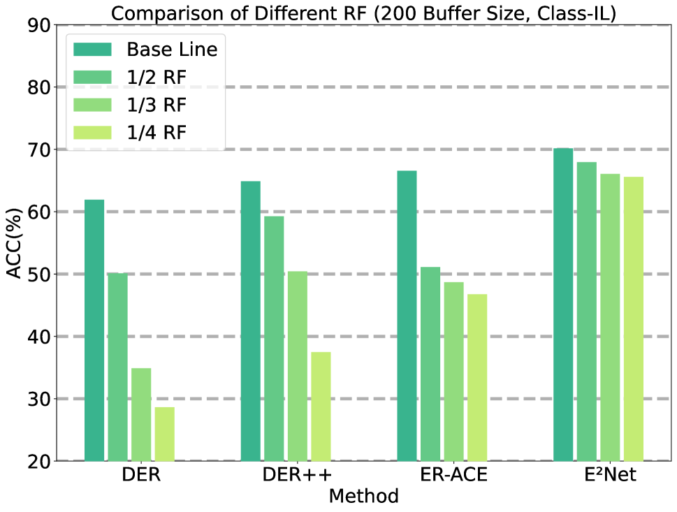
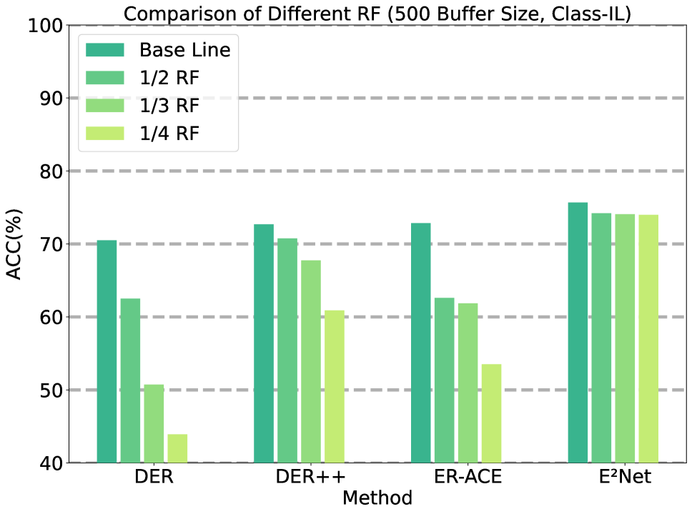
Rehearsal Frequency

To mitigate heightened computational complexity in rehearsal methods and enhance computing resource efficiency, we opted to decrease the Rehearsal Frequency (RF) during our experimentation. Figure 4 (a) and (b) showcase the achieved accuracy of different methods across various RF on S-CIFAR-10 dataset. Compared to other methods, E²Net exhibits a considerably smaller impact when RF are reduced. Notably, at a buffer size of 500 and 200, our method demonstrated a mere 1.68% and 4.58% decrease in accuracy when the RF was reduced to one-fourth of its original value. This indicates the robustness and effectiveness of our method in handling reduced RF while minimizing the impact on overall accuracy.⁵⁵5We offer additional experimental results concerning rehearsal frequency in the Appendix E.3.

Training Time

Minimizing overall processing time is crucial when dealing with data streams to ensure that training keeps pace with the rate at which data becomes available to the stream. To assess the performance of E²Net, as well as other rehearsal methods, we measure the wall-clock time upon completion of the final task. Figure 4 (c) illustrates the overall processing time measured on the S-CIFAR-10 dataset. The results demonstrate that our method achieves comparable processing time to DER++ and ER-ACE while achieving higher accuracy. By reducing rehearsal frequency, our method can achieve the shortest processing time and achieve higher computational efficiency.

Edge device Results

Method	S-CIFAR-10
Method	Class-IL	Task-IL
DER	61.02	90.86
DER++	64.53	91.54
E²Net w/ 1/4 RF	66.17	92.40
E²Net	70.25	93.80

Table 3: Comparison of Different Methods for S-CFAR-10 Dataset on the Nvidia Jetson TX2.

To demonstrate the practical potential of our method, we conducted evaluations on real edge devices. Table 3 presents the average accuracy of various methods on the Nvidia Jetson TX2. It is evident that our method achieves the highest accuracy, and there is no significant decline in accuracy on the edge device, showcasing the promising practical applicability of our method.

5 Conclusion

To optimize resource utilization efficiency and attain elevated accuracy within a shorter processing time, we propose Elastic Expansion Network, a resource-efficient CL method. E²Net selects the representative network from the search space at each task boundary to form candidate networks. These candidate networks effectively capture the essence of the working network and can be considered as its core components. During the training process of new tasks, we employ the Representative Network Distillation to facilitate knowledge transfer, effectively addressing the issue of forgetting previous task knowledge. To optimize rehearsal efficiency, we introduce the Subnet Constraint Experience Replay method to store and replay samples from data streams based on representative network’s sizes, thereby enhancing the performance of E²Net. Comprehensive experimentation across diverse benchmark datasets and environments substantiates E²Net’s effectiveness in mitigating forgetting. As a main limitation, E²Net makes a assumption about task boundaries. This encourages further research for future real-world applications. If fortunate enough to be accepted, we will release all the source code.

References

Aljundi et al. (2018) Aljundi, R.; Babiloni, F.; Elhoseiny, M.; Rohrbach, M.; and Tuytelaars, T. 2018. Memory Aware Synapses: Learning What (Not) to Forget. In Ferrari, V.; Hebert, M.; Sminchisescu, C.; and Weiss, Y., eds., Computer Vision – ECCV 2018, volume 11207, 144–161. Cham: Springer International Publishing. ISBN 9783030012182 9783030012199.
Aljundi et al. (2019) Aljundi, R.; Lin, M.; Goujaud, B.; and Bengio, Y. 2019. Gradient Based Sample Selection for Online Continual Learning. In Neural Information Processing Systems.
Arani, Sarfraz, and Zonooz (2022) Arani, E.; Sarfraz, F.; and Zonooz, B. 2022. Learning Fast, Learning Slow: A General Continual Learning Method Based on Complementary Learning System. ArXiv.
Atkinson et al. (2018) Atkinson, C.; McCane, B.; Szymanski, L.; and Robins, A. 2018. Pseudo-Recursal: Solving the Catastrophic Forgetting Problem in Deep Neural Networks. ArXiv.
Buzzega et al. (2020) Buzzega, P.; Boschini, M.; Porrello, A.; Abati, D.; and Calderara, S. 2020. Dark Experience for General Continual Learning: A Strong, Simple Baseline. ArXiv.
Caccia et al. (2021) Caccia, L.; Aljundi, R.; Tuytelaars, T.; Pineau, J.; and Belilovsky, E. 2021. Reducing representation drift in online continual learning. arXiv preprint arXiv:2104.05025, 1(3).
Cai, Gan, and Han (2019) Cai, H.; Gan, C.; and Han, S. 2019. Once for All: Train One Network and Specialize It for Efficient Deployment. ArXiv.
Cha, Lee, and Shin (2021) Cha, H.; Lee, J.; and Shin, J. 2021. Co2L: Contrastive Continual Learning. 2021 IEEE/CVF International Conference on Computer Vision (ICCV), 9496–9505.
Chaudhry et al. (2018a) Chaudhry, A.; Dokania, P. K.; Ajanthan, T.; and Torr, P. H. S. 2018a. Riemannian Walk for Incremental Learning: Understanding Forgetting and Intransigence. In Ferrari, V.; Hebert, M.; Sminchisescu, C.; and Weiss, Y., eds., Computer Vision – ECCV 2018, volume 11215, 556–572. Cham: Springer International Publishing. ISBN 9783030012519 9783030012526.
Chaudhry et al. (2021) Chaudhry, A.; Gordo, A.; Dokania, P.; Torr, P.; and Lopez-Paz, D. 2021. Using Hindsight to Anchor Past Knowledge in Continual Learning. Proceedings of the AAAI Conference on Artificial Intelligence, 35(8): 6993–7001.
Chaudhry et al. (2018b) Chaudhry, A.; Ranzato, M.; Rohrbach, M.; and Elhoseiny, M. 2018b. Efficient Lifelong Learning with A-GEM. ArXiv.
Chaudhry et al. (2019) Chaudhry, A.; Rohrbach, M.; Elhoseiny, M.; Ajanthan, T.; Dokania, P.; Torr, P. H. S.; and Ranzato, M. 2019. Continual Learning with Tiny Episodic Memories. ArXiv.
Delange et al. (2021) Delange, M.; Aljundi, R.; Masana, M.; Parisot, S.; Jia, X.; Leonardis, A.; Slabaugh, G.; and Tuytelaars, T. 2021. A Continual Learning Survey: Defying Forgetting in Classification Tasks. IEEE Transactions on Pattern Analysis and Machine Intelligence, 1–1.
Ebrahimi et al. (2020) Ebrahimi, S.; Meier, F.; Calandra, R.; Darrell, T.; and Rohrbach, M. 2020. Adversarial Continual Learning. In Vedaldi, A.; Bischof, H.; Brox, T.; and Frahm, J.-M., eds., Computer Vision – ECCV 2020, volume 12356, 386–402. Cham: Springer International Publishing. ISBN 9783030586201 9783030586218.
Golkar, Kagan, and Cho (2019) Golkar, S.; Kagan, M.; and Cho, K. 2019. Continual Learning via Neural Pruning. ArXiv.
Gurbuz and Dovrolis (2022) Gurbuz, M. B.; and Dovrolis, C. 2022. NISPA: Neuro-Inspired Stability-Plasticity Adaptation for Continual Learning in Sparse Networks.
He et al. (2016) He, K.; Zhang, X.; Ren, S.; and Sun, J. 2016. Deep Residual Learning for Image Recognition. 2016 IEEE Conference on Computer Vision and Pattern Recognition (CVPR), 770–778.
Ke, Liu, and Huang (2021) Ke, Z.; Liu, B.; and Huang, X. 2021. Continual Learning of a Mixed Sequence of Similar and Dissimilar Tasks. ArXiv.
Kirkpatrick et al. (2017) Kirkpatrick, J.; Pascanu, R.; Rabinowitz, N.; Veness, J.; Desjardins, G.; Rusu, A. A.; Milan, K.; Quan, J.; Ramalho, T.; Grabska-Barwinska, A.; Hassabis, D.; Clopath, C.; Kumaran, D.; and Hadsell, R. 2017. Overcoming Catastrophic Forgetting in Neural Networks. Proceedings of the National Academy of Sciences, 114(13): 3521–3526.
Krizhevsky (2009) Krizhevsky, A. 2009. Learning Multiple Layers of Features from Tiny Images.
Le and Yang (2015) Le, Y.; and Yang, X. S. 2015. Tiny ImageNet Visual Recognition Challenge.
Li et al. (2022) Li, J.; Ji, Z.; Wang, G.; Wang, Q.; and Gao, F. 2022. Learning from Students: Online Contrastive Distillation Network for General Continual Learning. In Proceedings of the Thirty-First International Joint Conference on Artificial Intelligence, 3215–3221. Vienna, Austria: International Joint Conferences on Artificial Intelligence Organization. ISBN 978-1-956792-00-3.
Li et al. (2019) Li, X.; Zhou, Y.; Wu, T.; Socher, R.; and Xiong, C. 2019. Learn to Grow: A Continual Structure Learning Framework for Overcoming Catastrophic Forgetting. In International Conference on Machine Learning.
Li and Hoiem (2016) Li, Z.; and Hoiem, D. 2016. Learning Without Forgetting. In Leibe, B.; Matas, J.; Sebe, N.; and Welling, M., eds., Computer Vision – ECCV 2016, volume 9908, 614–629. Cham: Springer International Publishing. ISBN 9783319464923 9783319464930.
Lin et al. (2021) Lin, J.; Chen, W.-M.; Cai, H.; Gan, C.; and Han, S. 2021. MCUNetV2: Memory-Efficient Patch-based Inference for Tiny Deep Learning. ArXiv.
Loo, Swaroop, and Turner (2020) Loo, N.; Swaroop, S.; and Turner, R. E. 2020. Generalized Variational Continual Learning. ArXiv.
Lopez-Paz and Ranzato (2017) Lopez-Paz, D.; and Ranzato, M. 2017. Gradient Episodic Memory for Continual Learning. In NIPS.
Mallya and Lazebnik (2018) Mallya, A.; and Lazebnik, S. 2018. PackNet: Adding Multiple Tasks to a Single Network by Iterative Pruning. In 2018 IEEE/CVF Conference on Computer Vision and Pattern Recognition, 7765–7773. Salt Lake City, UT: IEEE. ISBN 9781538664209.
McCloskey and Cohen (1989) McCloskey, M.; and Cohen, N. J. 1989. Catastrophic Interference in Connectionist Networks: The Sequential Learning Problem. In Psychology of Learning and Motivation, volume 24, 109–165. Elsevier. ISBN 9780125433242.
Prabhu, Torr, and Dokania (2020) Prabhu, A.; Torr, P. H. S.; and Dokania, P. K. 2020. GDumb: A Simple Approach That Questions Our Progress in Continual Learning. In Vedaldi, A.; Bischof, H.; Brox, T.; and Frahm, J.-M., eds., Computer Vision – ECCV 2020, volume 12347, 524–540. Cham: Springer International Publishing. ISBN 978-3-030-58535-8 978-3-030-58536-5.
Ramapuram, Gregorova, and Kalousis (2020) Ramapuram, J.; Gregorova, M.; and Kalousis, A. 2020. Lifelong generative modeling. Neurocomputing, 404: 381–400.
Rebuffi et al. (2017) Rebuffi, S.-A.; Kolesnikov, A.; Sperl, G.; and Lampert, C. H. 2017. iCaRL: Incremental Classifier and Representation Learning. In 2017 IEEE Conference on Computer Vision and Pattern Recognition (CVPR), 5533–5542. Honolulu, HI: IEEE. ISBN 9781538604571.
Riemer et al. (2018) Riemer, M.; Cases, I.; Ajemian, R.; Liu, M.; Rish, I.; Tu, Y.; and Tesauro, G. 2018. Learning to Learn without Forgetting By Maximizing Transfer and Minimizing Interference. ArXiv.
Rusu et al. (2016) Rusu, A. A.; Rabinowitz, N. C.; Desjardins, G.; Soyer, H.; Kirkpatrick, J.; Kavukcuoglu, K.; Pascanu, R.; and Hadsell, R. 2016. Progressive Neural Networks. ArXiv.
Schwarz et al. (2018) Schwarz, J.; Czarnecki, W. M.; Luketina, J.; Grabska-Barwinska, A.; Teh, Y.; Pascanu, R.; and Hadsell, R. 2018. Progress & Compress: A Scalable Framework for Continual Learning. In International Conference on Machine Learning.
Serrà et al. (2018) Serrà, J.; Surís, D.; Miron, M.; and Karatzoglou, A. 2018. Overcoming Catastrophic Forgetting with Hard Attention to the Task. In International Conference on Machine Learning.
Shin et al. (2017) Shin, H.; Lee, J. K.; Kim, J.; and Kim, J. 2017. Continual Learning with Deep Generative Replay. In NIPS.
Shokri and Shmatikov (2015) Shokri, R.; and Shmatikov, V. 2015. Privacy-Preserving Deep Learning. In Proceedings of the 22nd ACM SIGSAC Conference on Computer and Communications Security, 1310–1321. Denver Colorado USA: ACM. ISBN 9781450338325.
Sokar, Mocanu, and Pechenizkiy (2021) Sokar, G.; Mocanu, D. C.; and Pechenizkiy, M. 2021. SpaceNet: Make Free Space for Continual Learning. Neurocomputing, 439: 1–11.
Wang et al. (2020) Wang, Z.; Jian, T.; Chowdhury, K.; Wang, Y.; Dy, J.; and Ioannidis, S. 2020. Learn-Prune-Share for Lifelong Learning. In 2020 IEEE International Conference on Data Mining (ICDM), 641–650. Sorrento, Italy: IEEE. ISBN 9781728183169.
Wang et al. (2022) Wang, Z.; Zhang, Z.; Ebrahimi, S.; Sun, R.; Zhang, H.; Lee, C.-Y.; Ren, X.; Su, G.; Perot, V.; Dy, J.; and Pfister, T. 2022. DualPrompt: Complementary Prompting for Rehearsal-free Continual Learning. arXiv.
Wortsman et al. (2020) Wortsman, M.; Ramanujan, V.; Liu, R.; Kembhavi, A.; Rastegari, M.; Yosinski, J.; and Farhadi, A. 2020. Supermasks in Superposition. ArXiv.
Wu et al. (2019) Wu, Y.; Chen, Y.; Wang, L.; Ye, Y.; Liu, Z.; Guo, Y.; and Fu, Y. 2019. Large Scale Incremental Learning. In 2019 IEEE/CVF Conference on Computer Vision and Pattern Recognition (CVPR), 374–382. Long Beach, CA, USA: IEEE. ISBN 9781728132938.
Yan et al. (2022) Yan, Q.; Gong, D.; Liu, Y.; Van Den Hengel, A.; and Shi, J. Q. 2022. Learning Bayesian Sparse Networks with Full Experience Replay for Continual Learning. In 2022 IEEE/CVF Conference on Computer Vision and Pattern Recognition (CVPR), 109–118. New Orleans, LA, USA: IEEE. ISBN 9781665469463.
Yan, Xie, and He (2021) Yan, S.; Xie, J.; and He, X. 2021. DER: Dynamically Expandable Representation for Class Incremental Learning. In 2021 IEEE/CVF Conference on Computer Vision and Pattern Recognition (CVPR), 3013–3022. Nashville, TN, USA: IEEE. ISBN 9781665445092.
Yoon et al. (2017) Yoon, J.; Yang, E.; Lee, J.; and Hwang, S. J. 2017. Lifelong Learning with Dynamically Expandable Networks. ArXiv.
Yu et al. (2020) Yu, L.; Twardowski, B.; Liu, X.; Herranz, L.; Wang, K.; Cheng, Y.; Jui, S.; and Van De Weijer, J. 2020. Semantic Drift Compensation for Class-Incremental Learning. In 2020 IEEE/CVF Conference on Computer Vision and Pattern Recognition (CVPR), 6980–6989. Seattle, WA, USA: IEEE. ISBN 9781728171685.
Yu et al. (2022) Yu, L. L.; Hu, T.; Hong, L.; Liu, Z.; Weller, A.; and Liu, W. 2022. Continual Learning by Modeling Intra-Class Variation. Trans. Mach. Learn. Res., 2023.
Zenke, Poole, and Ganguli (2017) Zenke, F.; Poole, B.; and Ganguli, S. 2017. Continual Learning Through Synaptic Intelligence. Proceedings of machine learning research.
Zhao et al. (2022) Zhao, T.; Wang, Z.; Masoomi, A.; and Dy, J. 2022. Deep Bayesian Unsupervised Lifelong Learning. Neural Networks, 149: 95–106.

Appendix A Subnet Constraint Experience Replay

A.1 Sampling Algorithm

Here, we provide the sampling algorithm for the SCER. This algorithm effectively manages the memory buffer base on the subnet constraints, ensuring that valuable experiences are retained.

Algorithm 2 SCER Algorithm

Input: Memory Buffer

\mathcal{M}

, Memory Budget

\mathcal{B}

, Number of seen examples

N

, Representative Network parameter quantity

|\psi_{arch_{i}}|

, Working Network parameter quantity

|\theta|

, Selected example

(x,y)

\mathcal{B}>N

then

\mathcal{M}[N]\leftarrow(x,y)

\rhd

Memory is not full

else

k=\text{{randomInteger}}~{}(\min=0,\max=N)

i=\text{{random}}~{}(\min=0,\max=1)

i<\textit{exp}(-\alpha\frac{|\psi_{arch_{i}}|}{|\theta|})

then

k<\mathcal{B}

then

\mathcal{M}[k]\leftarrow(x,y)

\rhd

Select a sample to remove

end if

return

\theta

A.2 Sample preservation probability in the SCER method

Here we will use mathematical induction to calculate the probability of retaining the sample in the buffer (Eq. (10) in the main paper). For the first $\mathcal{B}$ samples $x_{1},x_{2},\ldots,x_{\mathcal{B}}$ , we will keep them in the buffer and $p(x_{1}\textit{ is retained})=p(x_{2}\textit{ is retained})=\ldots=p(x_{\mathcal{B}}\textit{ is retained})=1$ . For the k-th $(k>\mathcal{B})$ sample, we keep it with a probability of $p(x_{k})=\textit{exp}(-\alpha\frac{|\psi_{arch_{i}}|}{|\theta|})\frac{\mathcal{B}}{k}$ (which only means it is retained this time). So the probability of being retained in the first $\mathcal{B}$ samples $x_{r}(r\in 1:\mathcal{B})$ can be expressed as follows:

		$\displaystyle p(x_{r}\textit{ is retained})=$
		$\displaystyle p(x_{r}\textit{ was retained in the previous round})\times$
		$\displaystyle(p(x_{k}\textit{ is discarded})+p(x_{k}\textit{ is retained})\times p(x_{r}\textit{ not replaced}))$

Theorem 1.

For any positive integer $k(\mathcal{B}<k)$ , the following equation holds:

p(x_{r})=\prod_{n=\mathcal{B}+1}^{k}\frac{n\textit{exp}(\alpha\frac{|\psi_{arch_{i}}|}{|\theta|})-1}{n\textit{exp}(\alpha\frac{|\psi_{arch_{i}}|}{|\theta|})}

We will prove this equation using mathematical induction.

Base Step: When $k=\mathcal{B}+1$ , the sum on the left-hand side is $1\times((1-\textit{exp}(-\alpha\frac{|\psi_{arch_{i}}|}{|\theta|})\frac{\mathcal{B}}{\mathcal{B}+1}))+\textit{exp}(-\alpha\frac{|\psi_{arch_{i}}|}{|\theta|})\frac{\mathcal{B}}{\mathcal{B}+1}\times\frac{\mathcal{B}-1}{\mathcal{B}})=\frac{(\mathcal{B}+1)\textit{exp}(\alpha\frac{|\psi_{arch_{i}}|}{|\theta|})-1}{(\mathcal{B}+1)\textit{exp}(\alpha\frac{|\psi_{arch_{i}}|}{|\theta|})}$ , and the right-hand side evaluates to $\frac{(\mathcal{B}+1)\textit{exp}(\alpha\frac{|\psi_{arch_{i}}|}{|\theta|})-1}{(\mathcal{B}+1)\textit{exp}(\alpha\frac{|\psi_{arch_{i}}|}{|\theta|})}$ as well. Therefore, the equation holds.

Inductive Hypothesis: Assume that the equation holds for $k=m$ , i.e., $p(x_{r})=\prod_{n=\mathcal{B}+1}^{m}\frac{n\textit{exp}(\alpha\frac{|\psi_{arch_{i}}|}{|\theta|})-1}{n\textit{exp}(\alpha\frac{|\psi_{arch_{i}}|}{|\theta|})}$ .

Inductive Step: We need to show that the equation also holds for $k=m+1$ . We can expand the sum on the left-hand side as:

		$\displaystyle p(x_{r})=p(x_{r}\textit{ was retained in the previous round})\times$
		$\displaystyle((1-\textit{exp}(-\alpha\frac{\|\psi_{arch_{i}}\|}{\|\theta\|})\frac{\mathcal{B}}{m+1}))+$
		$\displaystyle\textit{exp}(-\alpha\frac{\|\psi_{arch_{i}}\|}{\|\theta\|})\frac{\mathcal{B}}{m+1}\times\frac{\mathcal{B}-1}{\mathcal{B}})$

Using the inductive hypothesis, $p(x_{r}\textit{ was retained in the previous round})$ is equal to $\prod_{n=\mathcal{B}+1}^{m}\frac{n\textit{exp}(\alpha\frac{|\psi_{arch_{i}}|}{|\theta|})-1}{n\textit{exp}(\alpha\frac{|\psi_{arch_{i}}|}{|\theta|})}$ . Thus, we can rewrite the above expression as:

\prod_{n=\mathcal{B}+1}^{m+1}\frac{n\textit{exp}(\alpha\frac{|\psi_{arch_{i}}|}{|\theta|})-1}{n\textit{exp}(\alpha\frac{|\psi_{arch_{i}}|}{|\theta|})}

Simplifying, we get:

p(x_{r})=\prod_{n=\mathcal{B}+1}^{m+1}\frac{n\textit{exp}(\alpha\frac{|\psi_{arch_{i}}|}{|\theta|})-1}{n\textit{exp}(\alpha\frac{|\psi_{arch_{i}}|}{|\theta|})}

This proves that the equation holds for $k=m+1$ .

By the principle of mathematical induction, the equation holds for any positive integer $n$ .

Figure 5 illustrates the probability of storing individual samples in a buffer under the SCER method, with the parameters $|\mathcal{D}|=1000$ and $\mathcal{B}=200$ .

Appendix B Experiment Details

B.1 Datasets

Split CIFAR-10 and Split CIFAR-100 (Krizhevsky 2009) consist of 5 and 20 tasks, each including 2 and 5 classes. Split Tiny ImageNet dataset is constructed by partitioning the original Tiny ImageNet dataset (Le and Yang 2015), which consists of 200 classes, into 10 tasks. Each task contains 20 classes. For Domain Incremental Learning (Domain-IL), previous research (Yan et al. 2022) often relied on Permuted MNIST (Kirkpatrick et al. 2017) and Rotated MNIST datasets (Lopez-Paz and Ranzato 2017). However, these tasks were relatively simple, resulting in the adoption of simplistic base network architectures. Therefore, the number and performance of representative networks searched in the CNS method are greatly limited. As a result, the focus of E²Net was primarily on Task-IL and Class-IL, where the diversity of subnets could be more comprehensively explored.

B.2 Evaluation Metrics

We use the following two metrics to measure the performance of various methods:

ACC_{t}=\frac{1}{t}\sum_{\tau=1}^{t}R_{t,\tau}

(12)

F_{t}=\frac{1}{t-1}\sum_{j=1}^{t-1}\max_{i\in\{1,\ldots,t-1\}}(R_{i,j}-R_{t,j}),

(13)

We denote the classification accuracy on the $\tau$ -th task after training on the t-th task as $R_{t,\tau}$ . A higher ACC value indicates superior model performance, while a lower F value signifies enhanced anti-forgetting efficacy of the model.

B.3 Implementation Details

For the CIFAR and Tiny ImageNet datasets, we adopted a standard ResNet18 (He et al. 2016) architecture without pretraining as the baseline, following the method taken in (Rebuffi et al. 2017).

In line with (Buzzega et al. 2020), we employ random crops and horizontal flips as data augmentation techniques for both examples from the current task and the replay buffer. It is important to note that data augmentation imposes an implicit constraint on the network.

All models are trained using the Stochastic Gradient Descent (SGD) optimizer and the batch size is fixed at 32. The details of other hyperparameters can be found in Appendix C and Appendix D. In the Split Tiny ImageNet setting, the models are trained for 100 epochs. As for the Split CIFAR-10 and Split CIFAR-100 settings, the models are trained for 50 epochs in each phase. Each batch comprises a combination of half the samples from the new task and half the samples from the buffer. At the end of each batch, the buffer is updated using the proposed SCER. When the rehearsal frequency is set to $1/2$ , the calculation of $\mathcal{L}_{\text{CE-M}}$ (Eq. (2) in the main paper) for backpropagation will occur only once every two batches. To ensure the scalability of the search space, we set $s_{t}\geq 1$ (Eq. (3) in the main paper).

Appendix C Hyperparameter Selection

Method	Buffer	Split Tiny ImageNet	Buffer	Split CIFAR-10
SGD	-	lr: $0.03$	-	lr: $0.1$
oEWC	-	lr: $0.03$ $\lambda$ : $90$ $\gamma$ : $1.0$	-	lr: $0.03$ $\lambda$ : $10$ $\gamma$ : $1.0$
SI	-	lr: $0.03$ c: $1.0$ $\xi$ : $0.9$	-	lr: $0.03$ c: $0.5$ $\xi$ : $1.0$
LwF	-	lr: $0.01$ $\alpha$ : $1$ T: $2.0$	-	lr: $0.03$ $\alpha$ : $0.5$ T: $2.0$
ER	200	lr: $0.1$	200	lr: $0.1$
	500	lr: $0.03$	500	lr: $0.1$
GEM			200	lr: $0.03$ $\gamma$ : $0.5$
			500	lr: $0.03$ $\gamma$ : $0.5$
A-GEM	200	lr: $0.01$	200	lr: $0.03$
	500	lr: $0.01$	500	lr: $0.03$
iCaRL	200	lr: $0.03$ wd: $10^{-5}$	200	lr: $0.1$ wd: $10^{-5}$
	500	lr: $0.03$ wd: $10^{-5}$	500	lr: $0.1$ wd: $10^{-5}$
GSS			200	lr: $0.03$ $gmbs$ : $32$ $nb$ : $1$
			500	lr: $0.03$ $gmbs$ : $32$ $nb$ : $1$
HAL			200	lr: $0.03$ $\lambda$ : $0.2$ $\beta$ : $0.5$
				$\gamma$ : $0.1$
			500	lr: $0.03$ $\lambda$ : $0.1$ $\beta$ : $0.3$
				$\gamma$ : $0.1$
DER	200	lr: $0.03$ $\alpha$ : $0.1$	200	lr: $0.03$ $\alpha$ : $0.3$
	500	lr: $0.03$ $\alpha$ : $0.1$	500	lr: $0.03$ $\alpha$ : $0.3$
DER++	200	lr: $0.03$ $\alpha$ : $0.1$ $\beta$ : $1.0$	200	lr: $0.03$ $\alpha$ : $0.1$ $\beta$ : $0.5$
	500	lr: $0.03$ $\alpha$ : $0.2$ $\beta$ : $0.5$	500	lr: $0.03$ $\alpha$ : $0.2$ $\beta$ : $0.5$
C $o^{2}$ L	200	lr: $0.03$ $\kappa$ : $0.1$ $\kappa^{*}$ : $0.1$	200	lr: $0.03$ $\kappa$ : $0.2$ $\kappa^{*}$ : $0.01$
		$\eta$ : $0.1$ $\tau$ : $0.5$ $epoch$ : $50$		$\eta$ : $0.5$ $\tau$ : $0.5$ $epoch$ : $100$
	500	lr: $0.03$ $\kappa$ : $0.1$ $\kappa^{*}$ : $0.1$	500	lr: $0.03$ $\kappa$ : $0.2$ $\kappa^{*}$ : $0.01$
		$\eta$ : $0.1$ $\tau$ : $0.5$ $epoch$ : $50$		$\eta$ : $0.5$ $\tau$ : $0.5$ $epoch$ : $100$
ER-ACE	200	lr: $0.1$ $\lambda$ : $2$	200	lr: $0.1$ $\lambda$ : $2$
	500	lr: $0.1$ $\lambda$ : $2$	500	lr: $0.1$ $\lambda$ : $2$

Method	Buffer	Split CIFAR-100
DER	100	lr: $0.03$ $\alpha$ : $0.1$
	200	lr: $0.03$ $\alpha$ : $0.1$
	500	lr: $0.03$ $\alpha$ : $0.1$
DER++	100	lr: $0.03$ $\alpha$ : $0.1$ $\beta$ : $1.0$
	200	lr: $0.03$ $\alpha$ : $0.1$ $\beta$ : $1.0$
	500	lr: $0.03$ $\alpha$ : $0.2$ $\beta$ : $0.5$
C $o^{2}$ L	100	lr: $0.03$ $\kappa$ : $0.2$ $\kappa^{*}$ : $0.01$
		$\eta$ : $0.5$ $\tau$ : $0.5$
	200	lr: $0.03$ $\kappa$ : $0.2$ $\kappa^{*}$ : $0.01$
		$\eta$ : $0.5$ $\tau$ : $0.5$
	500	lr: $0.03$ $\kappa$ : $0.2$ $\kappa^{*}$ : $0.01$
		$\eta$ : $0.5$ $\tau$ : $0.5$
ER-ACE	100	lr: $0.1$ $\lambda$ : $2$
	200	lr: $0.1$ $\lambda$ : $2$
	500	lr: $0.1$ $\lambda$ : $2$

Table 4: Hyperparameters selected for our experiments.

Table 4 presents the selected optimal hyperparameter combinations for each method in the main paper. The hyperparameters include the learning rate (lr), batch size (bs), and minibatch size (mbs) for rehearsal-based methods. Other symbols correspond to specific methods. It should be noted that the batch size and minibatch size are held constant at 32 for all Continual Learning benchmarks.

Appendix D Hyperparameter Sensitivity

Method	S-CIFAR-10
Method	Class-IL		Task-IL
Buffer Size	200	500	200	500
$\alpha=0.125$	68.16	74.92	93.41	94.74
$\alpha=0.25$	68.53	74.46	93.33	94.41
$\alpha=0.375$	69.44	75.04	93.64	94.54
$\alpha=0.5$	69.33	75.68	93.65	94.81
$\alpha=0.625$	68.97	75.66	93.66	94.97
$\alpha=0.75$	70.04	75.10	93.94	94.90
$\alpha=0.875$	70.06	74.95	93.71	94.93
$\alpha=1$	69.22	74.90	93.84	94.79
$\lambda=0.01$	68.18	75.16	93.60	94.59
$\lambda=0.025$	69.35	74.97	93.71	94.78
$\lambda=0.05$	70.16	75.66	93.75	94.95
$\lambda=0.075$	68.93	75.46	93.60	94.88
$\lambda=0.2$	68.85	74.93	93.71	94.83
$\lambda=0.5$	68.90	74.85	93.88	94.39

Table 5: Average Accuracy of E²Net on different values of hyperparameters. For a given hyperparameter in the table, all the other hyperparameters are set to their optimal values.

In Table 5, we report the performance of E²Net against a range of hyperparameters. $\alpha$ (Eq. (9) in the main paper) controls the subsequent impact of network size on SCER. A larger $\alpha$ value leads to a smaller number of samples retained by the network. $\lambda$ (Eq. (11) in the main paper) controls the distillation effect of the network on model training. A larger $\lambda$ value reduces the likelihood of the working network forgetting previous tasks, but it also makes learning new tasks more challenging. After conducting experiments, we found that the best results can be achieved when $\alpha=0.75$ and $\lambda=0.05$ and E²Net is not sensitive to the choice of hyperparameters.

Appendix E Additional Results

In this section, we present supplementary results for the experiments outlined in Sec. 4.3.

E.1 Forgetting

Method	S-CIFAR-10
Method	Class-IL		Task-IL
E²Net w/o BUF	28.37		71.85
Buffer Size	200	500	200	500
GEM	82.61 $\pm$ 1.6	74.31 $\pm$ 4.62	9.27 $\pm$ 2.07	9.12 $\pm$ 0.21
iCaRL	28.72 $\pm$ 0.49	25.71 $\pm$ 1.10	2.63 $\pm$ 3.48	2.66 $\pm$ 2.47
ER	61.24 $\pm$ 2.62	74.35 $\pm$ 0.07	7.08 $\pm$ 0.64	3.54 $\pm$ 0.35
A-GEM	95.73 $\pm$ 0.20	94.01 $\pm$ 1.16	16.39 $\pm$ 0.86	14.26 $\pm$ 4.18
GSS	75.25 $\pm$ 4.07	62.88 $\pm$ 2.67	8.56 $\pm$ 1.78	7.73 $\pm$ 3.99
DER	40.76 $\pm$ 0.42	26.74 $\pm$ 0.15	6.57 $\pm$ 0.20	4.56 $\pm$ 0.45
DER++	32.59 $\pm$ 2.32	22.38 $\pm$ 4.41	5.16 $\pm$ 0.21	4.66 $\pm$ 1.15
HAL	69.11 $\pm$ 4.21	62.21 $\pm$ 4.34	12.26 $\pm$ 0.02	5.41 $\pm$ 1.10
ER-ACE	35.79 $\pm$ 3.19	24.51 $\pm$ 2.19	6.92 $\pm$ 1.16	4.07 $\pm$ 0.08
E²Net (ours)	23.54 $\pm$ 2.17	16.68 $\pm$ 3.42	4.19 $\pm$ 1.13	1.84 $\pm$ 0.137

Table 6: Forgetting results on S-CIFAR-10 dataset.

Table 6 presents the Forgetting of all tasks after training. Our method exhibits the lowest forgetting, demonstrating the effectiveness of E²Net in preserving previous knowledge, rather than solely focusing on improving the accuracy of subsequent tasks.

E.2 Ablation Study

Method	S-CIFAR-10
Method	Class-IL	Task-IL
RND w/o Expansion	20.16	71.15
RND w/ Linear	25.62	68.08
RND w/ Cos	28.37	71.85

Table 7: Comparison of Different Expansion Methods on S-CIFAR-10 dataset.

Representative Network Distillation Module

We investigated the influence of different search space expansion methods on RND without a buffer. Table 7 presents the results obtained by enabling all search spaces at any task boundary (RND w/o Expansion), linearly expanding the search space (RND w/ Linear), and cosine expanding the search space (RND w/ Cos). The findings demonstrate that cosine expansion of the search space significantly improves the method’s performance. Allowing all search spaces from the beginning causes the method to quickly saturate, while linear expansion restricts the method’s initial search capabilities. Both scenarios result in a decline in method performance. These experiments provide valuable insights into the significance of the RND and the impact of different search space expansion methods on the overall performance of the method.

Candidate Networks Selection

In the absence of CNS, we default to selecting the largest network in the current search space as the representative network. However, this method does not consider the varying additional parameters required by different tasks. Similar tasks often require fewer additional parameters, indicating a higher degree of similarity between the representative networks. On the other hand, tasks with significant differences require more additional parameters, representing larger representative network differences. By incorporating CNS, the method can automatically identify the similarity between tasks and adjust the selection of representative networks accordingly to improve performance. Without CNS, the expansion of multiple search spaces requires more stringent rationality requirements and necessitates stronger theoretical support.

Subnet Constraint Experience Replay

Figure 6 illustrates the accuracy of the method for each task on the S-CIFAR-100 dataset. By incorporating the SCER module, the E²Net method achieves more balanced learning of previous knowledge, resulting in improved performance.

E.3 Rehearsal Frequency

Figure 7 illustrates the variations in the average accuracy of the method under distinct RF conditions. Remarkably, in both Task-IL and Class-IL, our method demonstrates the slowest decline in accuracy with decreasing RF. This feature grants E²Net an elastic rehearsal frequency design, enabling dynamic selection of the overall processing time and average accuracy. Figure 8 illustrates the correlation between accuracy and the processing time across different methods. Through dynamic processing time and average accuracy adjustment, our method can cater to a broader range of application scenarios.

E2Net: Resource-Efficient Continual Learning with Elastic Expansion Network

Abstract

1 Introduction

2 Related Work

Regularization-based methods

Architecture-based methods

Rehearsal-based methods

3 Elastic Expansion Network

3.1 Overview

3.2 Search Space Formulation

3.3 Candidate Networks Selection

3.4 Representative Network Distillation

3.5 Subnet Constraint Experience Replay

3.6 The Overall Loss

4 Experiments

4.1 Dataset and Hardware

4.2 Experimental Setup

Evaluation protocol.

Baselines.

4.3 Experimental Results

Class-IL and Task-IL settings with low buffer size

Class-IL and Task-IL settings without buffer

Dataset for 20-task setting

4.4 Ablation Study

4.5 Quantitative Study

Rehearsal Frequency

Training Time

Edge device Results

5 Conclusion

References

Appendix A Subnet Constraint Experience Replay

A.1 Sampling Algorithm

A.2 Sample preservation probability in the SCER method

Theorem 1.

Appendix B Experiment Details

B.1 Datasets

B.2 Evaluation Metrics

B.3 Implementation Details

Appendix C Hyperparameter Selection

Appendix D Hyperparameter Sensitivity

Appendix E Additional Results

E.1 Forgetting

E.2 Ablation Study

Representative Network Distillation Module

Candidate Networks Selection

Subnet Constraint Experience Replay

E.3 Rehearsal Frequency

E²Net: Resource-Efficient Continual Learning with Elastic Expansion Network