DyRoNet: Dynamic Routing and Low-Rank Adapters for Autonomous Driving Streaming Perception
Abstract
The advancement of autonomous driving systems hinges on the ability to achieve low-latency and high-accuracy perception. To address this critical need, this paper introduces Dynamic Routering Network (DyRoNet), a low-rank enhanced dynamic routing framework designed for streaming perception in autonomous driving systems. DyRoNet integrates a suite of pre-trained branch networks, each meticulously fine-tuned to function under distinct environmental conditions. At its core, the framework offers a speed router module, developed to assess and route input data to the most suitable branch for processing. This approach not only addresses the inherent limitations of conventional models in adapting to diverse driving conditions but also ensures the balance between performance and efficiency. Extensive experimental evaluations demonstrating the adaptability of DyRoNet to diverse branch selection strategies, resulting in significant performance enhancements across different scenarios. This work not only establishes a new benchmark for streaming perception but also provides valuable engineering insights for future work.111Project: https://tastevision.github.io/DyRoNet/
1 Introduction
In autonomous driving systems, it is crucial to achieve low-latency and high-precision perception. Traditional object detection algorithms [40], while effective in various contexts, often confront the challenge of latency due to inherent computational delays. This lag between algorithmic processing and real-world states can lead to notable discrepancies between predicted and actual object locations. Such latency issues have been extensively reported and are known to significantly impact the decision-making process in autonomous driving systems [4].
Addressing these challenges, the concept of streaming perception has been introduced as a response [20]. This perception task aims to predict “future” results by accounting for the delays incurred during the frame processing stage. Unlike traditional methods that primarily focus on detection at a given moment, streaming perception transcends this limitation by anticipating future environmental states, and aligning perceptual outputs closer to real-time dynamics. This new paradigm is key in addressing the critical gap between real-time processing and real-world changes, thereby enhancing the safety and reliability of autonomous driving systems [23].
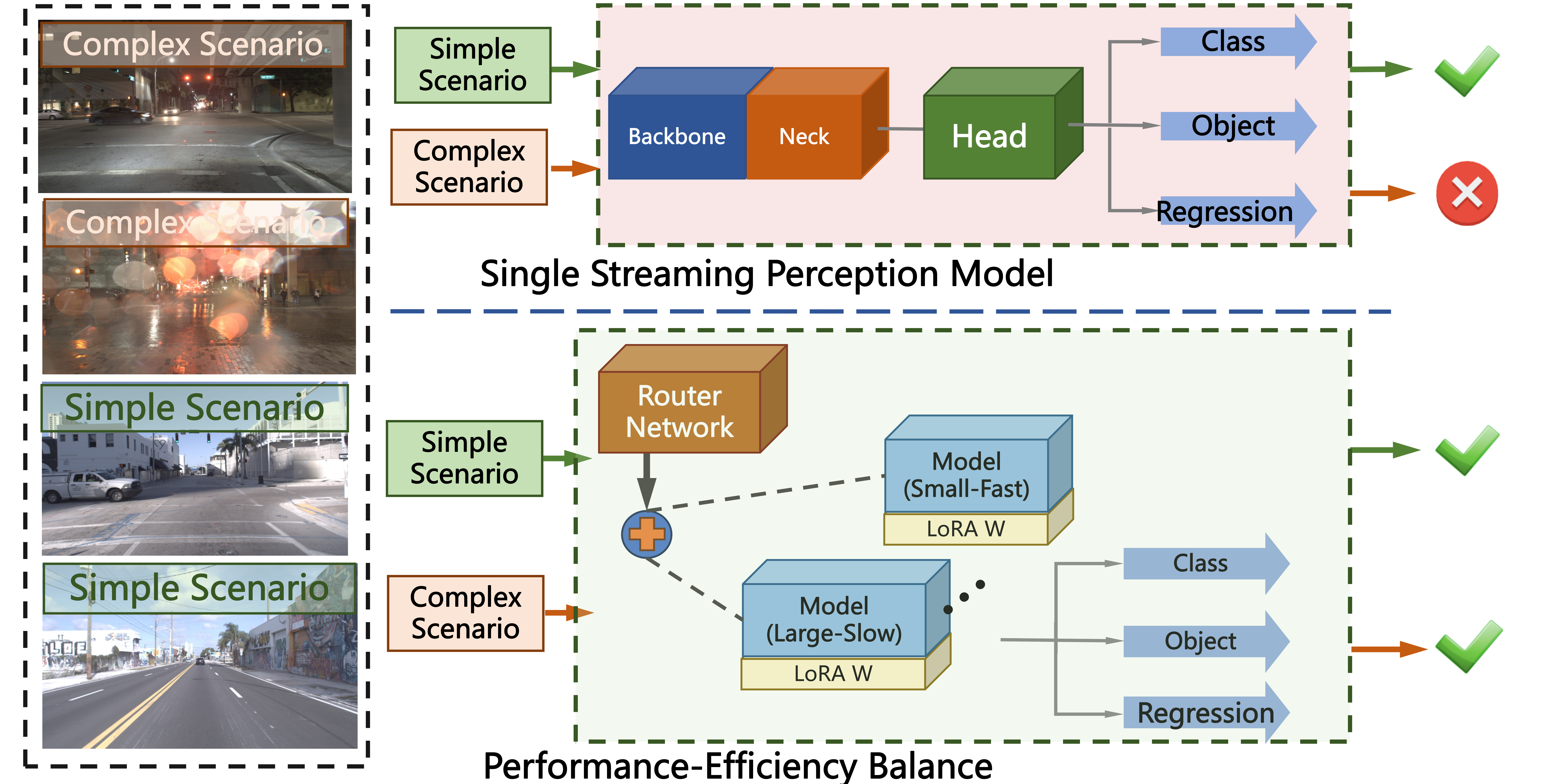
Although the existing streaming approach seems promising, it still faces contradictions in real-world scenarios. These contradictions primarily stem from the diverse and unpredictable nature of driving environments. The factors such as camera motion, weather conditions, lighting variations, and the presence of small objects seriously impact the performance of perception measures, leading to fluctuations that challenge their robustness and reliability (see Sec. 3.1). This complexity in real-world scenarios underscores the limitations of a single, uniform model, which often struggles to adapt to the varied demands of different driving conditions [8]. In general, the challenges of streaming perception mainly include:
(1) Diverse Scenario Distribution: Autonomous driving environments are inherently complex and dynamic, showing a myriad of scenarios that a single perception model may not adequately address (see Fig. 1). The need to customize perception algorithms to specific environmental conditions, while ensuring that these models operate cohesively, poses a significant challenge. As discussed in Sec. 3.1, adapting models to various scenarios without compromising their core functionality is a crucial aspect of streaming perception.
(2) Performance-Efficiency Balance: To our knowledge, the integration of both large and small-scale models is essential to handle the varying complexities encountered in different driving scenes. The large models, while potentially more accurate, may suffer from increased latency, whereas smaller models may offer faster inference at the cost of reduced accuracy. Balancing performance and efficiency, therefore, becomes a challenging task. In Sec. 3.1, we explore the strategies for optimizing this balance, exploring how different model architectures can be effectively utilized to enhance streaming perception.
Generally speaking, these challenges highlight the demand for streaming perception. As we study in Sec. 3.1, addressing the diverse scenario distribution and achieving an optimal balance between performance and efficiency are key to advancing the state-of-the-art in autonomous driving. To address the intricate challenges presented by real-world streaming perception, we introduce DyRoNet, a framework designed to enhance dynamic routing capabilities in autonomous driving systems. DyRoNet stands as a low-rank enhanced dynamic routing framework, specifically crafted to cater to the requirements of streaming perception. It encapsulates a suite of pre-trained branch networks, each meticulously fine-tuned to optimally function under distinct environmental conditions. A key component of DyRoNet is the speed router module, ingeniously developed to assess and efficiently route input to the optimal branch, as detailed in Sec. 3.2. To sum up, the contributions are listed as:
-
•
We emphasize the impact of environmental speed as a key determinant of streaming perception. Through analysis of various environmental factors, our research highlights the imperative need for adaptive perception responsive to dynamic conditions.
-
•
By utilizing a variety of streaming perception techniques, DyRoNet provides the speed router as a major invention. This component dynamically determines the best route for handling each input, ensuring efficiency and accuracy in perception. The ability to adapt and be versatile is demonstrated by this dynamic route-choosing mechanism.
-
•
Extensive experimental evaluations have demonstrated that DyRoNet is capable of adapting to diverse branch selection strategies, resulting in a substantial enhancement of performance across various branch structures. This not only validates the framework’s wide-ranging applicability but also confirms its effectiveness in handling different real-world scenarios.
2 Related Work
This section revisits developments in streaming perception and dynamic neural networks, highlighting differences from our proposed DyRoNet framework. While existing methods have made progress, limitations persist in addressing real-world autonomous driving complexity.
2.1 Streaming Perception
The existing streaming perception methods fall into three main categories. (1) The initial methods focused on single-frame, with models like YOLOv5 [15] and YOLOX [6] achieving real-time performance. However, lacking motion trend capture, they struggle in dynamic scenarios. (2) The recent approaches incorporated current and historical frames, like StreamYOLO [35] building on YOLOX with dual-flow fusion. LongShortNet [19] used longer histories and diverse fusion. DAMO-StreamNet [10] added asymmetric distillation and deformable convolutions to improve large object perception. (3) Recognizing the limitations of single models, current methods explore dynamic multi-model systems. One approach [7] adapts models to environments via reinforcement learning. DaDe [14] extends StreamYOLO by calculating delays to determine frame steps. A later version [13] added multi-branch prediction heads. Beyond 2D detection, streaming perception expands into optical flow, tracking, and 3D detection, with innovations in metrics and benchmarks [32, 25, 30]. Distinct from these existing approaches, our proposed method, DyRoNet, introduces a low-rank enhanced dynamic routing mechanism specifically designed for streaming perception. DyRoNet stands out by integrating a suite of advanced branch networks, each fine-tuned for specific environmental conditions. Its key innovation lies in the speed router module, which not only routes input data efficiently but also dynamically adapts to the diverse and unpredictable nature of real-world driving scenarios.
2.2 Dynamic Neural Networks
Dynamic Neural Networks (DNNs) feature adaptive network selection, outperforming static models in efficiency and performance [9, 17, 36]. The existing research primarily focuses on structural design for core deep learning tasks like image classification [12, 31, 29]. DNNs follow two approaches: (1) Multi-branch models [1, 3, 26, 28, 24, 33, 18] rely on a lightweight router assessing inputs to direct them to appropriate branches, enabling tailored computation. (2) By generating new weights based on inputs [34, 5, 27, 39], these models dynamically alter computations to match diverse needs. DNN applications expand beyond conventional tasks. In object detection, DynamicDet [21] categorizes inputs and processes them through distinct branches. This illustrates DNNs’ broader applicability and potential for dynamic environments.
3 Proposed Method
This section outlines the framework of our proposed DyRoNet. Beginning with its underlying motivation and the critical factors driving its design, we subsequently provide an overview of its architecture and training process.
3.1 Motivation for DyRoNet
Autonomous driving faces variability from weather, scene complexity, and vehicle velocity. By strategically analyzing key factors and routing logic, this section details the rationale behind the proposed DyRoNet.
Analysis of Influential Factors. Statistical analysis of the Argoverse-HD dataset [20] underscores the profound influence of environmental dynamics on the effectiveness of streaming perception. While weather inconsistently impacts accuracy, suggesting the presence of other influential factors (see Appendix A.1), fluctuations in the object count show limited correlation with performance degradation (see Appendix A.2). Conversely, the presence of small objects across various scenes poses a significant challenge for detection, especially under varying motion states (see Appendix A.3). Notably, disparities in performance are most pronounced across different environmental motion states (see Appendix A.4), thereby motivating the need for a dynamic, velocity-aware routing mechanism in DyRoNet.
Rationale for Dynamic Routing. Analysis reveals that StreamYOLO’s reliance on a single historical frame falters at high velocities, in contrast to multi-frame models, highlighting a connection between speed and detection performance (see Tab. 2). Dynamic adaptation of frame history, based on vehicular speed, enables DyRoNet to strike a balance between accuracy and latency (see Sec. 4.3). Through first-order differences, the system efficiently switches models to align with environmental motions. Specifically, the dynamic routing is designed to select the optimal architecture based on the vehicle’s speed profile, ensuring precision at lower velocities for detailed perception and efficiency at higher speeds for swift response. These comprehensive analysis imforms DyRoNet as a robust solution for reliable perception across diverse autonomous driving scenarios.
3.2 Architecture of DyRoNet
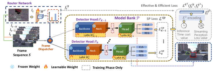
Overview of DyRoNet. The structure of DyRoNet, as depicted in Fig. 2, proposes a multi-branch structure. Each branch within DyRoNet framework functions as an independent streaming perception model, capable of processing both the current and historical frames. This dual-frame processing is central to DyRoNet’s capability, facilitating a nuanced understanding of temporal dynamics. Such a design is key in achieving a delicate balance between latency and accuracy, aspects crucial for real-time autonomous driving.
Mathematically, the core of DyRoNet lies the processing of a frame sequence, , where indicates the number of frames and the interval between successive frames. The framework process is formalized as:
where denotes a collection of streaming perception models, with each denoting an individual model within this suite. The architecture is further enhanced by incorporating a feature extractor and a perception head for each model. The Router Network, , is instrumental in selecting the most suitable streaming perception model for each specific scenario.
Correspondingly, the weights of DyRoNet are denoted by , where indicates the weights of the streaming perception model, relates to the Low-Rank Adaptation (LoRA) weights within each model, and pertains to the Router Network. The culmination of this process is the final output, , a compilation of feature maps. These maps can be further decoded through , revealing essential details like objects, categories, and locations.
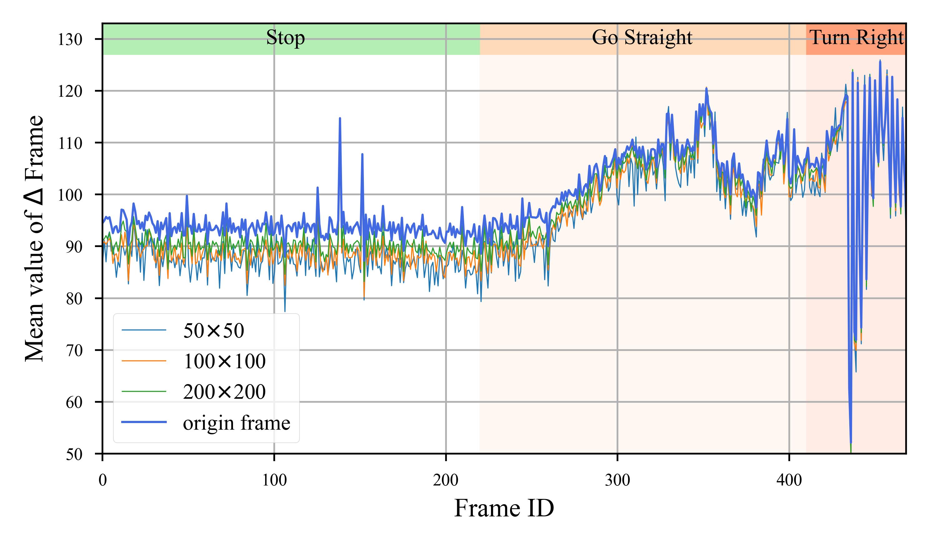
Router Network. The Router Network in DyRoNet plays a crucial role in understanding and classifying the dynamics of the environment. This module is designed for both environmental classification and branch decision-making. To effectively capture environmental speed, frame differences are employed as the input to the Router Network. As shown in Fig. 3, frame differences exhibit a high discriminative advantage for different environmental speeds.
Specifically, for frames at times and , represented as and respectively, the frame difference is computed as . The architecture of the Router Network, , is simple yet efficient. It consists of a single convolutional layer followed by a linear layer. The network’s output, denoted as , captures the essence of the environmental dynamics. Based on this output, the index of the optimal branch for processing the current input frame is determined through the following equation:
| (1) |
where is the index of the branch deemed most suitable for the current environmental context. Once is determined, the input frame is automatically routed to the corresponding branch by a dispatcher.
In particular, this strategy of using frame differences to gauge environmental speed is efficient. It offers a faster alternative to traditional methods such as optical flow fields. Moreover, it focuses on frame-level variations rather than the speed of individual objects, providing a more generalized representation of environmental dynamics. The sparsity of also contributes to the robustness of this method, reducing computational complexity and making the Router Network’s operations nearly negligible in the context of the overall model’s performance.
Model Bank & Dispatcher. The core of the DyRoNet framework is its model bank, which consists of an array of streaming perceptual models, denoted as . Typically, the selection of the most suitable model for processing a given input is intelligently managed by the Router Network. This process is formalized as , where Disp acts as a dispatcher, facilitating the dynamic selection of models from based on the input. The operational flow of DyRoNet can be mathematically defined as:
where symbolizes the Router Network, and refers to the frame difference, a key input for model selection. The weights and correspond to the selected streaming perception model and its LoRA parameters, respectively.
Note that the versatility of DyRoNet is further highlighted by its compatibility with a wide range of Streaming Perception models, even ones that rely solely on detectors [6]. To demonstrate the efficacy of DyRoNet, it has been evaluated using three contemporary streaming perception models: StreamYOLO [35], LongShortNet [19], and DAMO-StreamNet [10] (see Sec. 4.3). This Model Bank & Dispatcher strategy illustrates the adaptability and robustness of DyRoNet across different streaming perception scenarios.
Low-Rank Adaptation. A key challenge arises when fully fine-tuning individual branches, especially under the direction of Router Network. This strategy can lead to biases in the distribution of training data and inefficiencies in the learning process. Specifically, lighter branches may become predisposed to simpler cases, while more complex ones might be tailored to handle intricate scenarios, thereby heightening the risk of overfitting. Our experimental results, detailed in Sec. 4.3, support this observation.
To address these challenges, we have incorporated the LoRA [11] into DyRoNet. Within each model , initially pre-trained on a dataset, the key components are the convolution kernel and bias matrices, symbolized as . The rank of the LoRA module is defined as , a value significantly smaller than the dimensionality of , to ensure efficient adaptation. The update to the weight matrix adheres to a low-rank decomposition form, represented as .222Here, is a matrix in , and is in , ensuring that the rank remains much smaller than . This adaptation strategy allows for the original weights to remain fixed, while the low-rank components are trained and adjusted. The adaptation process is executed through the following projection:
| (2) |
where represents the input image or feature map, and . The matrices and start from an initialized state and are fine-tuned during adaptation. This approach maintains the general applicability of the model by fixing , while also enabling specialization within specific sub-domains, as determined by Router Network.
In DyRoNet, we employ for the LoRA module, though this can be adjusted based on specific requirements of the scenarios in question. This low-rank adaptation mechanism not only enhances the flexibility of the DyRoNet framework but also mitigates the risk of overfitting, ensuring that each branch remains efficient and effective in its designated role.
3.3 Training Details of DyRoNet
The training process of DyRoNet focuses on two primary goals: (1) Improving the performance of individual branches. The backpropagation only updates the chosen model’s weights in this step, enabling fine-tuning on segregated samples. (2) Achieving an optimal balance between accuracy and computational efficiency. This step only train the speed router while the remaining branches are frozen. This dual-objective framework is represented by the overall loss function:
| (3) |
where represents the streaming perception loss, and denotes the effective and efficient (E2) loss, which supervises branch selection.
Streaming Perception (SP) Loss. Each branch in DyRoNet is fine-tuned using its original loss function to maintain effectiveness. The router network is trained to select the optimal branch based on efficiency supervision. Let denote the logits produced by the -th branch and represent the corresponding ground-truth, where , , and are the classification, objectness, and regression logits, respectively. The streaming perception loss for each branch, , is defined as follows:
| (4) | ||||
where and are defined as Mean Square Error (MSE) loss functions, while is represented by the Generalized Intersection over Union (GIoU) loss.
Effective and Efficient (E2) Loss. During the training phase, streaming perception loss values from all branches are compiled into a vector , and inference time costs are aggregated into , with indicating the total number of branches in DyRoNet. To account for hardware variability, a normalized inference time vector is introduced. This vector is derived using the Softmax function to minimize the influence of hardware discrepancies. The representation for effective and efficient (E2) decision-making is defined as:
| (5) |
where denotes one-hot encoding, producing a boolean vector of length , with the value of at the index representing the estimated optimal branch at that moment. The E2 Loss is then formulated as:
| (6) |
where and represents the Kullback-Leibler divergence, utilized to constrain the distribution.
DyRoNet and relevant techniques. Although the structure of DyRoNet is somewhat similar to MoE[26, 37], in contrast, the gate network of MoE is not well-suited for streaming perception. This limitation has led to the development of speed router and the loss function. DyRoNet, for efficiency, chooses one model over MoE’s multiple experts, aligning with MoE in concept but differing in gate structure and selection strategy, making it unique for streaming contexts.
The speed router is inspired by Network Architecture Search (NAS). However, it uniquely addresses the challenge of streaming perception by transforming the search problem into an optimization of coded distances. The formulation of the loss function, , involves converting into a distribution via softmax, which is then combined with to determine the optimal model through an one-hot vector . This approach effectively simplifies the intricate problem of balancing accuracy and latency into a more tractable optimization task. Instead of employing NAS for loss search, our design is intricately linked to the specific needs of streaming perception, with KL divergence selected for its robustness in noisy situations[16]. This demonstrates the efficiency and innovation of our approach.
Overall, the process of training DyRoNet involves striking a meticulous balance between the SP loss, which ensures the efficacy of each branch, and the E2 loss, which optimizes efficiency. The primary objective of this training is to develop a model that not only delivers high accuracy in perception tasks but also operates within acceptable latency constraints, which is a critical requirement for real-time applications. This balanced approach enables DyRoNet to adapt dynamically to varying computational resources and environmental conditions, thereby maintaining optimal performance in diverse streaming perception scenarios.
4 Experiments
| Model | Random | MoE | DyRoNet | ||||||||
|---|---|---|---|---|---|---|---|---|---|---|---|
| Bank | latency | sAP | latency | sAP | latency | sAP | sAP50 | sAP75 | sAPs | sAPm | sAPl |
| 39.16 | 31.5 | 66.16 | 29.5 | 26.25 (-12.91) | 33.7 (+2.2) | 53.9 | 34.1 | 13.0 | 35.1 | 59.3 | |
| 24.04 | 33.2 | 70.19 | 29.5 | 29.35 (+5.31) | 36.9 (+3.7) | 58.2 | 37.5 | 14.8 | 37.4 | 64.2 | |
| 24.69 | 35.4 | 83.65 | 33.7 | 23.51 (-1.18) | 35.0 (-0.4) | 55.7 | 35.5 | 13.7 | 36.2 | 61.1 | |
| 24.79 | 31.8 | 128.74 | 29.8 | 21.47 (-3.32) | 30.5 (-1.3) | 51.2 | 30.2 | 11.3 | 31.1 | 56.1 | |
| 21.49 | 33.4 | 121.62 | 29.8 | 30.48 (+8.99) | 37.1 (+3.7) | 58.3 | 37.6 | 15.1 | 37.6 | 63.7 | |
| 24.75 | 35.6 | 136.66 | 34.1 | 29.05 (+4.30) | 36.9 (+1.3) | 58.2 | 37.4 | 14.9 | 37.5 | 63.3 | |
| 36.61 | 33.5 | 188.42 | 31.8 | 33.22 (-3.39) | 35.5 (+2.0) | 56.9 | 36.2 | 14.4 | 36.8 | 63.2 | |
| 35.12 | 34.5 | 188.57 | 31.8 | 39.60 (+4.48) | 37.8 (+3.3) | 59.1 | 38.7 | 16.1 | 39.0 | 64.2 | |
| 37.30 | 36.5 | 195.87 | 35.5 | 37.61 (+0.31) | 37.8 (+1.3) | 58.8 | 38.8 | 16.1 | 39.0 | 64.0 | |
| Methods | Latency (ms) | sAP |
| Non-real-time detector-based methods | ||
| Adaptive Streamer [7] | - | 21.3 |
| Streamer (S=600) [20] | - | 20.4 |
| Streamer (S=900) [20] | - | 18.2 |
| Streamer+AdaScale [7] | - | 13.8 |
| Real-time detector-based methods | ||
| DAMO-StreamNet-L [10] | 39.6 | 37.8 |
| LongShortNet-L [19] | 29.9 | 37.1 |
| StreamYOLO-L [35] | 29.3 | 36.1 |
| DAMO-StreamNet-M [10] | 33.5 | 35.7 |
| LongShortNet-M [19] | 25.1 | 34.1 |
| StreamYOLO-M [35] | 24.8 | 32.9 |
| DAMO-StreamNet-S [10] | 30.1 | 31.8 |
| LongShortNet-S [19] | 20.3 | 29.8 |
| StreamYOLO-S [35] | 21.3 | 28.8 |
| DyRoNet () | 37.61 (-1.99) | 37.8 (same) |
| DyRoNet () | 29.05 (-0.85) | 36.9 (-0.2) |
| DyRoNet () | 23.51 (-5.79) | 35.0 (-1.1) |
4.1 Dataset and Metric
Dataset. Argoverse-HD dataset [20] is utilized for our experiments, specifically designed for streaming perception in autonomous driving scenarios. It comprises high-resolution RGB images captured from urban city street, offering a realistic representation of diverse driving conditions. The dataset is structured into two main segments: a training set consisting of 65 video clips and a test set comprising 24 video clips. Each video clip in the dataset spans over 600 frames in average, contributing to a training set with approximately 39k frames and a test set containing around 15k frames. Notably, Argoverse-HD provides high-frame-rate (30fps) 2D object detection annotations, ensuring accuracy and reliability without relying on interpolated data.
Evaluation Metric. Streaming Average Precision (sAP) are adopted as the primary metric for performance evaluation, which is widely recognized for its effectiveness in streaming perception tasks [20]. It offers a comprehensive assessment by calculating the mean Average Precision (mAP) across various Intersection over Union (IoU) thresholds, ranging from 0.5 to 0.95. This metric allows us to evaluate detection performance across different object sizes, including large, medium, and small objects, providing a robust measurement in real-world streaming perception scenarios.
4.2 Implementation Details
We tested three state-of-the-art streaming perception models: StreamYOLO[35], LongShortNet[19], and DAMO-StreamNet[10]. These models, integral to the DyRoNet architecture, come with pre-trained parameters across three distinct scales: small (S), medium (M), and large (L), catering to a variety of processing requirements. In constructing the model bank for DyRoNet, we strategically selected different model configurations to evaluate performance across diverse scenarios. For instance, the notation DyRoNet () represents a configuration where DyRoNet employs the small (S) and medium (M) scales of DAMO-StreamNet as its two branches.333Similar notations are used for other model combinations, allowing for a systematic exploration of the framework’s adaptability and performance under varying computational constraints. All experiments were conducted on a high-performance computing platform equipped with Nvidia 3090Ti GPUs (x4), ensuring robust and reliable computational power to handle the intensive processing demands of the streaming perception models. This setup provided a consistent and controlled environment for evaluating the efficacy of DyRoNet across different model configurations, contributing to the thoroughness and validity of our results. For more implementation details, please refer to Appendix C.
4.3 Comparision with SOTA Methods
We compared DyRoNet with state-of-the-art methods to evaluate its performance. In this subsection, we directly copied the reported sAP performance from their original papers as their results, for fair comparison, we evaluated the latency of each real-time model on 1x RTX 3090. The performance comparison was conducted on the Argoverse-HD dataset [20]. An overview of the results reveals that our proposed DyRoNet with a model bank of DAMO-StreamNet series achieves 37.8% sAP in 37.61 ms latency, outperforming the current state-of-the-art methods in latency by a significant margin. This demonstrates the effectiveness of the systematic improvements in DyRoNet.
| Model Bank | Full (sAP) | LoRA (sAP) |
|---|---|---|
| 32.9 | 33.7 (+0.8) | |
| 36.1 | 36.9 (+0.8) | |
| 36.2 | 35.0 (-1.2) | |
| 29.0 | 30.5 (+1.5) | |
| 36.2 | 37.1 (+0.9) | |
| 36.3 | 36.9 (+0.6) | |
| 34.8 | 35.5 (+0.7) | |
| 31.1 | 37.8 (+6.7) | |
| 37.4 | 37.8 (+0.4) |
| Model Bank | sAP | ||||
|---|---|---|---|---|---|
| same model | 31.8 | 35.5 | - | 35.5 | |
| 31.8 | 37.8 | - | 37.8 | ||
| 35.5 | 37.8 | - | 37.8 | ||
| 29.8 | 34.1 | - | 30.5 | ||
| 29.8 | 37.1 | - | 37.1 | ||
| 34.1 | 37.1 | - | 36.9 | ||
| 29.5 | 33.7 | - | 33.7 | ||
| 29.5 | 36.9 | - | 36.9 | ||
| 33.7 | 36.9 | - | 35.0 | ||
| different model | + | 31.8 | 29.8 | - | 30.5 |
| + | 31.8 | 34.1 | - | 34.1 | |
| + | 31.8 | 37.1 | - | 31.8 | |
| + | 35.5 | 29.8 | - | 29.8 | |
| + | 37.8 | 29.8 | - | 29.8 | |
| same model | 31.8 | 35.5 | 37.8 | 37.7 | |
| 29.8 | 34.1 | 37.1 | 36.1 | ||
| 29.5 | 33.7 | 36.9 | 36.6 |
4.4 Inference Time
In this subsection, we conducted detailed experiments analyzing the trade-offs between DyRoNet’s inference time and performance under different model bank selection. It is notable that the latency of DyRoNet presented in Tab. 2 do not accurately reflect the real outperform. Due to the varying hardware platforms for measuring latency across methods, a fair comparison cannot be achieved. For instance, DAMO-StreamNet is tested on 1x V100. To address these differences, we conducted additional tests on a 1x RTX 3090, which highlight DyRoNet’s performance enhancements. Tab. 1 presents the latency comparison and highlights DyRoNet’s superior performance—maintaining competitive inference speed alongside accuracy gains versus the random and MoE approaches. Where the MoE predicts the weights of each branch via a gate module and then combines the output results accordingly. Specifically, DyRoNet achieves efficient speeds while preserving or enhancing performance. This balance enables meeting real-time needs without compromising perception quality, critical for autonomous driving where both factors are paramount. By validating effectiveness in inference time reductions and accuracy improvements, the results show the practicality and efficiency of DyRoNet’s dynamic model selection.
4.5 Ablation Study
Router Network. To validate the effectiveness of the Router Network based on frame difference, we conducted comparative experiments using frame difference , the current frame , and the concatenation of the consecutive frames as input modality of the Router Network. For comparison, a naive method of input guidance also employed: By calculating , the larger branch is selected if , otherwise the smaller branch is chosen. The results are presented in Tab. 6. For comparison, the Router Network only be trained in these experiments while the leftover parts be frozen.
It shows that using as input exhibits better performance than other methods (35.0 sAP of and 34.6 sAP of ). This indicates that utilizing offers significant advantages in comprehending and characterizing environmental speed. Conversely, it also underscores that employing single frames as input or using multiple frames as input renders the lightweight model bank selection model ineffective. Furthermore, the proportion of sample splits across branches can also illustrate the discriminative power with respect to environmental factors. For instance, the criterion resulting in a evenly spliting distribution (48.22% over train set and 49.85% over test set). Indicating the direct sample selection without router lacks estimation of environmental factors, thereby weakening its discriminative power.
In contrast, Tab.5 presents statistics indicating the router layer’s effectiveness in allocating samples to specific models and showcase its ability to strike a balance between latency and performance. This balance is crucial for streaming perception and underscores our contribution.
| Model | training time | inference time | ||
|---|---|---|---|---|
| Combination | Model 1 | Model 2 | Model 1 | Model 2 |
| SYOLO (M+L) | 37.53% | 62.47% | 94.67% | 5.33% |
| LSN (M+L) | 30.86% | 69.14% | 19.87% | 80.13% |
| DAMO (M+L) | 84.61% | 15.39% | 0.02% | 99.98% |
| Model | Input Modality / Criterion | |||
|---|---|---|---|---|
| Bank | (DyRoNet) | |||
| 33.7 | 33.7 | 31.5 | 32.6 | |
| 34.1 | 30.2 | 32.9 | 35.0 | |
| 33.7 | 33.7 | 34.2 | 34.6 | |
Branch Selection. Our research on streaming perception models has shown that configuring these models across varying scales can optimize their performance. We found that combining L and S models strikes an optimal balance, resulting in significant speed improvements. This conclusion is supported by the empirical evidence presented in Tab. 4, which clearly shows that the L+S model pairing outperforms both the L+S and L+M cases. Our findings highlight the importance of strategic model scaling in streaming perception and provide a framework for future model optimization in similar domains.
Fine-tuning Scheme. We contrasted the performance of direct fine-tuning with the LoRA fine-tuning strategy [38] for streaming perception models. Tab. 3 shows that LoRA fine-tuning surpasses direct fine-tuning, with the DAMO-Streamnet-based model bank configuration realizing an absolute gain of over 1.6%. This substantiates LoRA’s fine-tuning proficiency in circumventing the pitfalls of forgetting and data distribution bias inherent to direct fine-tuning. This result demonstrates that LoRA fine-tuning can effectively mitigate the overfitting while fine-tuning, leading to a stable performance improvement.
LoRA Rank. To assess the impact of LoRA ranks in DyRoNet, we conducted experiments with rank respectively. All experiments were train for 5 epochs between Router Network training and model bank fine-tuning. The results are presented in Tab. 7. It can be observed that the performance is better with compared to and , and only occupy 10% of the total model parameters. Therefore, based on these experiments, was selected as the default setting for our experiments. Although a smaller LoRA rank occupies fewer parameters, it leads to a rapid performance decay. The experimental results clearly demonstrate that with LoRA fine-tuning, it is possible to achieve superior performance than a single model while utilizing a smaller parameter footprint.
| Model Bank | Rank | branch 0 | branch 1 | after train | Param.(%) |
|---|---|---|---|---|---|
| 8 | 31.8 | 37.8 | 35.9 | 4.02 | |
| 16 | 31.8 | 37.8 | 35.9 | 7.73 | |
| 32 | 31.8 | 37.8 | 37.8 | 14.35 | |
| 8 | 29.8 | 37.1 | 30.6 | 5.48 | |
| 16 | 29.8 | 37.1 | 30.6 | 5.48 | |
| 32 | 29.8 | 37.1 | 36.9 | 10.39 | |
| 8 | 29.5 | 36.9 | 35.0 | 2.7 | |
| 16 | 29.5 | 36.9 | 35.0 | 5.38 | |
| 32 | 29.5 | 36.9 | 36.6 | 10.21 |
4.6 Extra Experiment on NuScenes-H dataset
To validate the DyRoNet on other dataset, we converted the 3D streaming perception dataset nuScenes-H[30] into 2D format. The experiment details are provided in the Appendix D. As shown in Tab. 8, DyRoNet consistently achieves better results than other branch fusion methods on nuScenes-H 2D dataset. It demonstrates DyRoNet’s advantages in branch fusion selection and its versatility.
| Model Bank | b1 | b2 | Random | MoE | DyRoNet |
|---|---|---|---|---|---|
| 6.9 | 9.2 | 8.1 | 6.9 | 8.9 | |
| 7.3 | 9.9 | 8.6 | 7.3 | 9.0 | |
| 8.9 | 9.6 | 9.2 | 8.9 | 9.3 | |
| 6.6 | 6.2 | 6.4 | 6.2 | 6.5 | |
| 9.1 | 9.3 | 9.2 | 9.1 | 9.3 | |
| 9.0 | 9.6 | 9.3 | 9.0 | 9.6 |
5 Conclusion
In conclusion, we present the Dynamic Routering Network (DyRoNet), a system that dynamically selects specialized detectors for varied environmental conditions with minimal computational overhead. Our Low-Rank Adapter mitigates distribution bias, thereby enhancing scene-specific performance. Experimental results validate DyRoNet’s state-of-the-art performance, offering a benchmark for streaming perception and insights for future research. In the future, DyRoNet’s principles will inform the development of more advanced, reliable systems.
Acknowledgments
Zhi-Qi Cheng’s research in this project was supported in part by the US Department of Transportation, Office of the Assistant Secretary for Research and Technology, under the University Transportation Center Program (Federal Grant Number 69A3551747111), and Intel and IBM Fellowships.
References
- [1] Babak Ehteshami Bejnordi, Tijmen Blankevoort, and Max Welling. Batch-shaping for learning conditional channel gated networks. In International Conference on Learning Representations, 2019.
- [2] Holger Caesar, Varun Bankiti, Alex H. Lang, Sourabh Vora, Venice Erin Liong, Qiang Xu, Anush Krishnan, Yu Pan, Giancarlo Baldan, and Oscar Beijbom. nuscenes: A multimodal dataset for autonomous driving. In Proceedings of the IEEE/CVF Conference on Computer Vision and Pattern Recognition, June 2020.
- [3] Shaofeng Cai, Yao Shu, and Wei Wang. Dynamic routing networks. In Proceedings of the IEEE/CVF Winter Conference on Applications of Computer Vision, pages 3588–3597, January 2021.
- [4] Li Chen, Penghao Wu, Kashyap Chitta, Bernhard Jaeger, Andreas Geiger, and Hongyang Li. End-to-end autonomous driving: Challenges and frontiers, 2023.
- [5] Yinpeng Chen, Xiyang Dai, Mengchen Liu, Dongdong Chen, Lu Yuan, and Zicheng Liu. Dynamic convolution: Attention over convolution kernels. In Proceedings of the IEEE/CVF Conference on Computer Vision and Pattern Recognition, June 2020.
- [6] Zheng Ge, Songtao Liu, Feng Wang, Zeming Li, and Jian Sun. Yolox: Exceeding yolo series in 2021. arXiv preprint arXiv:2107.08430, 2021.
- [7] Anurag Ghosh, Akshay Nambi, Aditya Singh, Harish Yvs, and Tanuja Ganu. Adaptive streaming perception using deep reinforcement learning. arXiv preprint arXiv:2106.05665, 2021.
- [8] Junyao Guo, Unmesh Kurup, and Mohak Shah. Is it safe to drive? an overview of factors, metrics, and datasets for driveability assessment in autonomous driving. IEEE Transactions on Intelligent Transportation Systems, 21(8):3135–3151, 2019.
- [9] Yizeng Han, Gao Huang, Shiji Song, Le Yang, Honghui Wang, and Yulin Wang. Dynamic neural networks: A survey. IEEE Transactions on Pattern Analysis and Machine Intelligence, 44(11):7436–7456, 2021.
- [10] Jun-Yan He, Zhi-Qi Cheng, Chenyang Li, Wangmeng Xiang, Binghui Chen, Bin Luo, Yifeng Geng, and Xuansong Xie. Damo-streamnet: Optimizing streaming perception in autonomous driving. In Proceedings of the Thirty-Second International Joint Conference on Artificial Intelligence, IJCAI-23, pages 810–818. International Joint Conferences on Artificial Intelligence Organization, 8 2023.
- [11] Edward J Hu, Yelong Shen, Phillip Wallis, Zeyuan Allen-Zhu, Yuanzhi Li, Shean Wang, Lu Wang, and Weizhu Chen. Lora: Low-rank adaptation of large language models. arXiv preprint arXiv:2106.09685, 2021.
- [12] Gao Huang, Danlu Chen, Tianhong Li, Felix Wu, Laurens van der Maaten, and Kilian Weinberger. Multi-scale dense networks for resource efficient image classification. In International Conference on Learning Representations, 2018.
- [13] Yihui Huang and Ningjiang Chen. Mtd: Multi-timestep detector for delayed streaming perception. In Chinese Conference on Pattern Recognition and Computer Vision, pages 337–349. Springer, 2023.
- [14] Wonwoo Jo, Kyungshin Lee, Jaewon Baik, Sangsun Lee, Dongho Choi, and Hyunkyoo Park. Dade: Delay-adoptive detector for streaming perception. arXiv preprint arXiv:2212.11558, 2022.
- [15] Glenn Jocher, Alex Stoken, Jirka Borovec, Ayush Chaurasia, Liu Changyu, Adam Hogan, Jan Hajek, Laurentiu Diaconu, Yonghye Kwon, Yann Defretin, et al. ultralytics/yolov5: v5. 0-yolov5-p6 1280 models, aws, supervise. ly and youtube integrations. Zenodo, 2021.
- [16] Taehyeon Kim et al. Comparing kullback-leibler divergence and mean squared error loss in knowledge distillation. In IJCAI, pages 2628–2635, 2021.
- [17] Jin-Peng Lan, Zhi-Qi Cheng, Jun-Yan He, Chenyang Li, Bin Luo, Xu Bao, Wangmeng Xiang, Yifeng Geng, and Xuansong Xie. Procontext: Exploring progressive context transformer for tracking. In IEEE International Conference on Acoustics, Speech and Signal Processing, pages 1–5. IEEE, 2023.
- [18] JunKyu Lee, Blesson Varghese, and Hans Vandierendonck. Roma: Run-time object detection to maximize real-time accuracy. In Proceedings of the IEEE/CVF Winter Conference on Applications of Computer Vision, pages 6405–6414, 2023.
- [19] Chenyang Li, Zhi-Qi Cheng, Jun-Yan He, Pengyu Li, Bin Luo, Hanyuan Chen, Yifeng Geng, Jin-Peng Lan, and Xuansong Xie. Longshortnet: Exploring temporal and semantic features fusion in streaming perception. In IEEE International Conference on Acoustics, Speech and Signal Processing, pages 1–5. IEEE, 2023.
- [20] Mengtian Li, Yu-Xiong Wang, and Deva Ramanan. Towards streaming perception. In Proceedings of the European Conference on Computer Vision, pages 473–488. Springer, 2020.
- [21] Zhihao Lin, Yongtao Wang, Jinhe Zhang, and Xiaojie Chu. Dynamicdet: A unified dynamic architecture for object detection. In Proceedings of the IEEE/CVF Conference on Computer Vision and Pattern Recognition, pages 6282–6291, June 2023.
- [22] Bharat Mahaur and KK Mishra. Small-object detection based on yolov5 in autonomous driving systems. Pattern Recognition Letters, 168:115–122, 2023.
- [23] Khan Muhammad, Amin Ullah, Jaime Lloret, Javier Del Ser, and Victor Hugo C de Albuquerque. Deep learning for safe autonomous driving: Current challenges and future directions. IEEE Transactions on Intelligent Transportation Systems, 22(7):4316–4336, 2020.
- [24] Jian-Jun Qiao, Zhi-Qi Cheng, Xiao Wu, Wei Li, and Ji Zhang. Real-time semantic segmentation with parallel multiple views feature augmentation. In ACM International Conference on Multimedia, pages 6300–6308, 2022.
- [25] Gur-Eyal Sela, Ionel Gog, Justin Wong, Kumar Krishna Agrawal, Xiangxi Mo, Sukrit Kalra, Peter Schafhalter, Eric Leong, Xin Wang, Bharathan Balaji, et al. Context-aware streaming perception in dynamic environments. In Proceedings of the European Conference on Computer Vision, pages 621–638. Springer, 2022.
- [26] Noam Shazeer, Azalia Mirhoseini, Krzysztof Maziarz, Andy Davis, Quoc Le, Geoffrey Hinton, and Jeff Dean. Outrageously large neural networks: The sparsely-gated mixture-of-experts layer. arXiv preprint arXiv:1701.06538, 2017.
- [27] Hang Su, Varun Jampani, Deqing Sun, Orazio Gallo, Erik Learned-Miller, and Jan Kautz. Pixel-adaptive convolutional neural networks. In Proceedings of the IEEE/CVF Conference on Computer Vision and Pattern Recognition, June 2019.
- [28] Hao Wang, Zhi-Qi Cheng, Jingdong Sun, Xin Yang, Xiao Wu, Hongyang Chen, and Yan Yang. Debunking free fusion myth: Online multi-view anomaly detection with disentangled product-of-experts modeling. In ACM International Conference on Multimedia, pages 3277–3286, 2023.
- [29] Xin Wang, Fisher Yu, Zi-Yi Dou, Trevor Darrell, and Joseph E. Gonzalez. Skipnet: Learning dynamic routing in convolutional networks. In Proceedings of the European Conference on Computer Vision, September 2018.
- [30] Xiaofeng Wang, Zheng Zhu, Yunpeng Zhang, Guan Huang, Yun Ye, Wenbo Xu, Ziwei Chen, and Xingang Wang. Are we ready for vision-centric driving streaming perception? the asap benchmark. In Proceedings of the IEEE/CVF Conference on Computer Vision and Pattern Recognition, pages 9600–9610, 2023.
- [31] Yulin Wang, Kangchen Lv, Rui Huang, Shiji Song, Le Yang, and Gao Huang. Glance and focus: a dynamic approach to reducing spatial redundancy in image classification. In H. Larochelle, M. Ranzato, R. Hadsell, M.F. Balcan, and H. Lin, editors, Advances in Neural Information Processing Systems, volume 33, pages 2432–2444. Curran Associates, Inc., 2020.
- [32] Zixiao Wang, Weiwei Zhang, and Bo Zhao. Estimating optical flow with streaming perception and changing trend aiming to complex scenarios. Applied Sciences, 13(6):3907, 2023.
- [33] Ran Xu, Fangzhou Mu, Jayoung Lee, Preeti Mukherjee, Somali Chaterji, Saurabh Bagchi, and Yin Li. Smartadapt: Multi-branch object detection framework for videos on mobiles. In Proceedings of the IEEE/CVF Conference on Computer Vision and Pattern Recognition, pages 2528–2538, 2022.
- [34] Brandon Yang, Gabriel Bender, Quoc V Le, and Jiquan Ngiam. Condconv: Conditionally parameterized convolutions for efficient inference. In H. Wallach, H. Larochelle, A. Beygelzimer, F. d'Alché-Buc, E. Fox, and R. Garnett, editors, Advances in Neural Information Processing Systems, volume 32. Curran Associates, Inc., 2019.
- [35] Jinrong Yang, Songtao Liu, Zeming Li, Xiaoping Li, and Jian Sun. Real-time object detection for streaming perception. In Proceedings of the IEEE/CVF Conference on Computer Vision and Pattern Recognition, pages 5385–5395, June 2022.
- [36] Ji Zhang, Xiao Wu, Zhi-Qi Cheng, Qi He, and Wei Li. Improving anomaly segmentation with multi-granularity cross-domain alignment. In ACM International Conference on Multimedia, pages 8515–8524, 2023.
- [37] Yanqi Zhou, Tao Lei, Hanxiao Liu, Nan Du, Yanping Huang, Vincent Zhao, Andrew M Dai, Quoc V Le, James Laudon, et al. Mixture-of-experts with expert choice routing. Advances in Neural Information Processing Systems, 35:7103–7114, 2022.
- [38] Jiawen Zhu, Zhi-Qi Cheng, Jun-Yan He, Chenyang Li, Bin Luo, Huchuan Lu, Yifeng Geng, and Xuansong Xie. Tracking with human-intent reasoning. arXiv preprint arXiv:2312.17448, 2023.
- [39] Xizhou Zhu, Han Hu, Stephen Lin, and Jifeng Dai. Deformable convnets v2: More deformable, better results. In Proceedings of the IEEE/CVF Conference on Computer Vision and Pattern Recognition, June 2019.
- [40] Zhengxia Zou, Keyan Chen, Zhenwei Shi, Yuhong Guo, and Jieping Ye. Object detection in 20 years: A survey. Proceedings of the IEEE, 2023.
DyRoNet: Dynamic Routing and Low-Rank Adapters for Autonomous Driving Streaming Perception
(Supplementary Material)
The appendix completes the main paper by providing in-depth research details and extended experimental results. The structure of the appendix is organized as follows:
- 1.
- 2.
- 3.
-
4.
Detailed Description of Experiments on nuScenes-H Dataset: Sec. D
Appendix A Factor Analysis in Streaming Perception
In development of DyRoNet, we undertook an extensive survey and analysis to identify key influencing factors in autonomous driving scenarios that could potentially impact streaming perception. This analysis utilized the Argoverse-HD dataset [20], a benchmark in the field of streaming perception. The primary goal of this factor analysis was to isolate the most critical factor affecting streaming perception performance. As elaborated in the main text, our comprehensive analysis led to the identification of the speed of the environment as the predominant factor. Consequently, DyRoNet is tailored to address this specific aspect. Our analysis focuses on four primary elements: weather conditions, object quantity, small object proportion, and environmental speed. We methodically examined each of these factors to evaluate their respective impacts on streaming perception within autonomous driving.
A.1 Impact of Weather Conditions
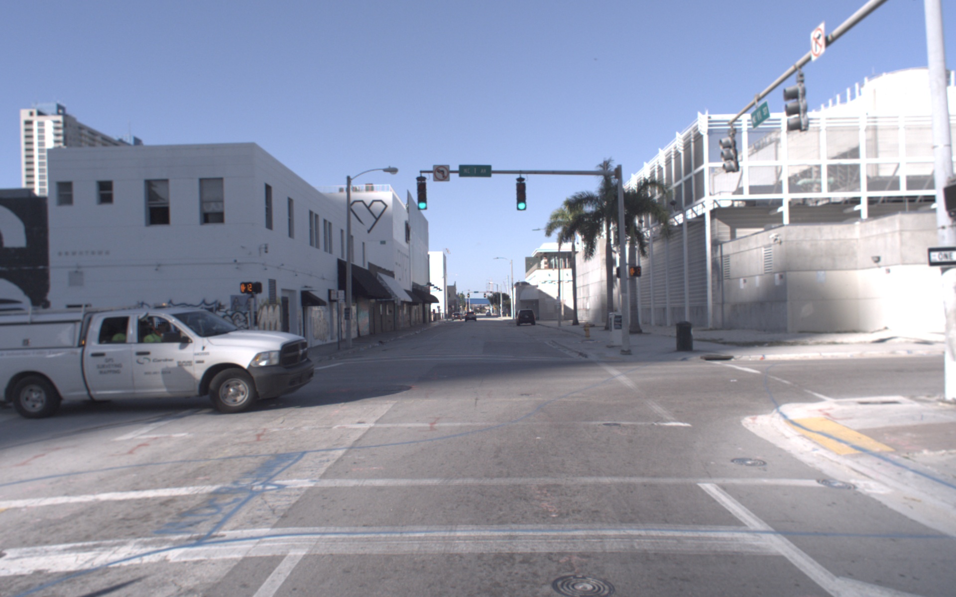
The Argoverse-HD dataset, comprising testing, training, and validation sets, includes a diverse range of weather conditions. Specifically, the dataset contains 24, 65, and 24 video segments in the testing, training, and validation sets, respectively, with frame counts ranging from 400 to 900 per segment. Tab. 9 details the distribution of various weather types across these subsets. Fig. 4 provides visual examples of different weather conditions captured in the dataset. A clear variation in visual clarity and perception difficulty is observable under different conditions, with scenarios like Sunny + Day or Cloudy + Day appearing visually more challenging compared to Rainy + Night.
To evaluate the impact of weather conditions on streaming perception, we conducted tests using a range of pre-trained models from StreamYOLO [35], LongShortNet [19], and DAMO-StreamNet [10], employing various scales and settings. The results, presented in Tab. 10, indicate that performance is generally better during Day conditions compared to Night. This confirms that weather conditions indeed influence streaming perception.
However, it’s noteworthy that even within the same weather conditions, model performance varies significantly, with accuracy ranging from below 10% to above 70%. Fig. 5 illustrates this point by comparing frames from two video segments (Clip ids: 00c561 and 395560) under identical weather conditions, where the performance difference of the same model on these segments is as high as 32.1%. This observation suggests the presence of other critical environmental factors that affect streaming perception, indicating that weather, while influential, is not the sole determinant of model performance.
| test | train | val | |
|---|---|---|---|
| Sunny + Day | 8 | 34 | 8 |
| Cloudy + Day | 13 | 27 | 15 |
| Rainy + Day | 1 | 1 | 0 |
| Rainy + Night | 1 | 0 | 0 |
| Sunny + Night | 1 | 3 | 1 |
| StreamYOLO | LongShortNet | DAMO-StreamNet | ||||||||||||
| Clip ID | Weather | s 1x | m 1x | l 1x | l 2x | l still | s 1x | m 1x | l 1x | l high | s 1x | m 1x | l 1x | l high |
| 1d6767 | Cloudy + Day | 20.9 | 22.8 | 24.9 | 7.0 | 26.7 | 20.9 | 23.4 | 25.0 | 36.4 | 21.3 | 24.6 | 26.0 | 34.2 |
| 5ab269 | Cloudy + Day | 25.6 | 30.0 | 31.6 | 6.9 | 33.3 | 25.2 | 29.5 | 31.4 | 40.1 | 26.9 | 29.0 | 31.7 | 41.2 |
| 70d2ae | Cloudy + Day | 26.3 | 31.4 | 37.9 | 9.4 | 41.0 | 25.2 | 31.0 | 37.5 | 44.7 | 27.7 | 34.8 | 34.3 | 44.9 |
| 337375 | Cloudy + Day | 24.8 | 24.8 | 33.4 | 17.1 | 35.3 | 27.2 | 27.9 | 34.7 | 38.0 | 26.4 | 37.5 | 28.8 | 39.1 |
| 7d37fc | Cloudy + Day | 32.5 | 36.4 | 41.5 | 15.5 | 42.1 | 33.6 | 37.7 | 40.8 | 45.8 | 35.2 | 40.1 | 39.4 | 45.7 |
| f1008c | Cloudy + Day | 38.6 | 42.0 | 44.4 | 11.3 | 46.2 | 40.0 | 40.4 | 45.3 | 50.3 | 39.1 | 42.4 | 45.8 | 54.1 |
| f9fa39 | Cloudy + Day | 35.7 | 39.5 | 41.8 | 9.9 | 48.1 | 33.2 | 39.8 | 42.9 | 50.1 | 38.8 | 44.1 | 44.3 | 51.4 |
| cd6473 | Cloudy + Day | 40.0 | 45.7 | 44.0 | 11.3 | 52.7 | 36.6 | 47.3 | 47.3 | 54.0 | 40.2 | 44.6 | 47.9 | 54.7 |
| cb762b | Cloudy + Day | 36.4 | 41.3 | 44.3 | 10.8 | 44.8 | 36.9 | 41.4 | 44.4 | 57.7 | 40.9 | 44.8 | 43.7 | 57.6 |
| aeb73d | Cloudy + Day | 39.6 | 44.6 | 45.2 | 12.5 | 46.7 | 39.2 | 46.7 | 45.9 | 52.3 | 42.6 | 46.4 | 47.5 | 51.3 |
| cb0cba | Cloudy + Day | 48.3 | 47.5 | 52.1 | 13.8 | 50.9 | 46.0 | 47.5 | 50.4 | 55.5 | 47.1 | 47.7 | 51.5 | 59.4 |
| e9a962 | Cloudy + Day | 45.6 | 53.8 | 55.4 | 15.8 | 58.8 | 44.0 | 52.8 | 55.6 | 60.7 | 45.1 | 50.2 | 52.9 | 56.2 |
| 2d12da | Cloudy + Day | 50.8 | 56.5 | 56.2 | 11.9 | 58.8 | 48.5 | 54.6 | 56.6 | 59.1 | 53.1 | 54.8 | 57.5 | 63.8 |
| 85bc13 | Cloudy + Day | 56.2 | 56.8 | 60.1 | 19.5 | 62.1 | 55.3 | 58.2 | 59.2 | 63.5 | 54.9 | 58.3 | 59.6 | 67.3 |
| 00c561 | Sunny + Day | 16.2 | 19.0 | 20.5 | 5.1 | 22.2 | 17.6 | 20.1 | 20.2 | 26.4 | 17.9 | 19.3 | 21.5 | 25.2 |
| c9d6eb | Sunny + Day | 22.5 | 28.9 | 32.5 | 07.5 | 35.3 | 22.6 | 28.8 | 32.9 | 39.1 | 24.5 | 26.0 | 28.4 | 38.6 |
| cd5bb9 | Sunny + Day | 23.3 | 24.9 | 25.8 | 6.2 | 27.2 | 23.4 | 25.2 | 25.8 | 30.4 | 23.4 | 25.7 | 26.2 | 31.5 |
| 6db21f | Sunny + Day | 24.1 | 26.4 | 27.0 | 6.7 | 28.9 | 23.3 | 27.0 | 27.0 | 34.7 | 25.1 | 28.0 | 28.7 | 37.0 |
| 647240 | Sunny + Day | 27.1 | 29.3 | 31.2 | 07.8 | 34.1 | 26.5 | 30.1 | 31.5 | 38.8 | 26.9 | 32.0 | 32.0 | 38.4 |
| da734d | Sunny + Day | 30.2 | 33.4 | 37.0 | 8.8 | 39.9 | 29.2 | 34.4 | 37.5 | 42.6 | 34.2 | 35.7 | 38.2 | 43.1 |
| 5f317f | Sunny + Day | 31.9 | 42.3 | 45.9 | 8.9 | 50.1 | 32.8 | 42.0 | 46.1 | 51.2 | 40.0 | 44.6 | 47.0 | 54.0 |
| 395560 | Sunny + Day | 49.3 | 61.2 | 60.6 | 11.3 | 72.1 | 51.7 | 60.7 | 58.5 | 65.4 | 58.9 | 63.4 | 57.8 | 59.6 |
| b1ca08 | Sunny + Day | 60.0 | 62.1 | 68.4 | 22.4 | 67.9 | 61.7 | 61.4 | 67.7 | 70.6 | 59.6 | 65.0 | 67.7 | 68.6 |
| 033669 | Sunny + Night | 18.0 | 23.5 | 25.7 | 6.6 | 27.4 | 18.5 | 23.6 | 25.1 | 27.6 | 21.8 | 22.7 | 23.8 | 27.5 |
| Overall | – | 29.8 | 33.7 | 36.9 | 34.6 | 39.4 | 29.8 | 34.1 | 37.1 | 42.7 | 31.8 | 35.5 | 37.8 | 43.3 |
A.2 Analysis of Object Quantity Impact
To assess the impact of the number of objects on streaming perception, we conducted a statistical analysis of object counts per frame in the Argoverse-HD dataset, encompassing both training and validation sets. The results of this analysis are depicted in Fig 6, which showcases a histogram representing the distribution of the number of objects in individual frames. The variance in the distribution is notable, with values of for the training set and for the validation set, indicating significant fluctuation in the number of objects across frames. Additionally, as shown in Tab. 10, there is considerable variability in object counts across different video segments. This observation led us to further investigate the potential correlation between object quantity and model performance fluctuations.
To explore this correlation, we calculated the average number of objects per frame for each segment within the Argoverse-HD validation set. The findings, detailed in Tab. 11, include the average object counts alongside Spearman correlation coefficients, which measure the relationship between object quantity and model performance. The absolute values of these coefficients range from 1e-1 to 1e-2. This range of correlation coefficients suggests that the number of objects present in the environment does not exhibit a strong or significant correlation with the performance of streaming perception models. In other words, our analysis indicates that the sheer quantity of objects within the environment is not a predominant factor influencing the efficacy of streaming perception.
| Clip ID | Mean Obj | sYOLO | LSN | DAMO |
|---|---|---|---|---|
| 1d6767 | 35.30 | 20.9 | 20.9 | 21.3 |
| 7d37fc | 30.89 | 32.5 | 33.6 | 35.2 |
| da734d | 25.16 | 30.2 | 29.2 | 34.2 |
| cd6473 | 23.75 | 40.0 | 36.6 | 40.2 |
| 5ab269 | 23.37 | 25.6 | 25.2 | 26.9 |
| cb762b | 23.31 | 36.4 | 36.9 | 40.9 |
| f1008c | 23.08 | 38.6 | 40.0 | 39.1 |
| e9a962 | 21.58 | 45.6 | 44.0 | 45.1 |
| 70d2ae | 21.38 | 26.3 | 25.2 | 27.7 |
| 2d12da | 19.33 | 50.8 | 48.5 | 53.1 |
| 337375 | 18.19 | 24.8 | 27.2 | 26.4 |
| f9fa39 | 17.46 | 35.7 | 33.2 | 38.8 |
| aeb73d | 16.82 | 39.6 | 39.2 | 42.6 |
| 6db21f | 16.30 | 24.1 | 23.3 | 25.1 |
| 647240 | 14.18 | 27.1 | 26.5 | 26.9 |
| b1ca08 | 14.08 | 60.0 | 61.7 | 59.6 |
| 85bc13 | 12.06 | 56.2 | 55.3 | 54.9 |
| 033669 | 11.89 | 18.0 | 18.5 | 21.8 |
| 00c561 | 10.06 | 16.2 | 17.6 | 17.9 |
| cb0cba | 10.04 | 48.3 | 46.0 | 47.1 |
| 395560 | 10.00 | 49.3 | 51.7 | 58.9 |
| cd5bb9 | 8.95 | 23.3 | 23.4 | 23.4 |
| c9d6eb | 7.88 | 22.5 | 22.6 | 24.5 |
| 5f317f | 6.92 | 31.9 | 32.8 | 40.0 |
| Coefficient | – | 0.052 | 0.035 | -0.020 |
A.3 Analysis of the Proportion of Small Objects
The influence of small objects on perception models, particularly in autonomous driving scenarios, has been underscored in studies like [22] and [35]. In such scenarios, even minor shifts in viewing angles can cause notable relative displacement of small objects, posing a challenge for perception models in processing streaming data effectively. This observation prompted us to closely examine the proportion of small objects in the environment.
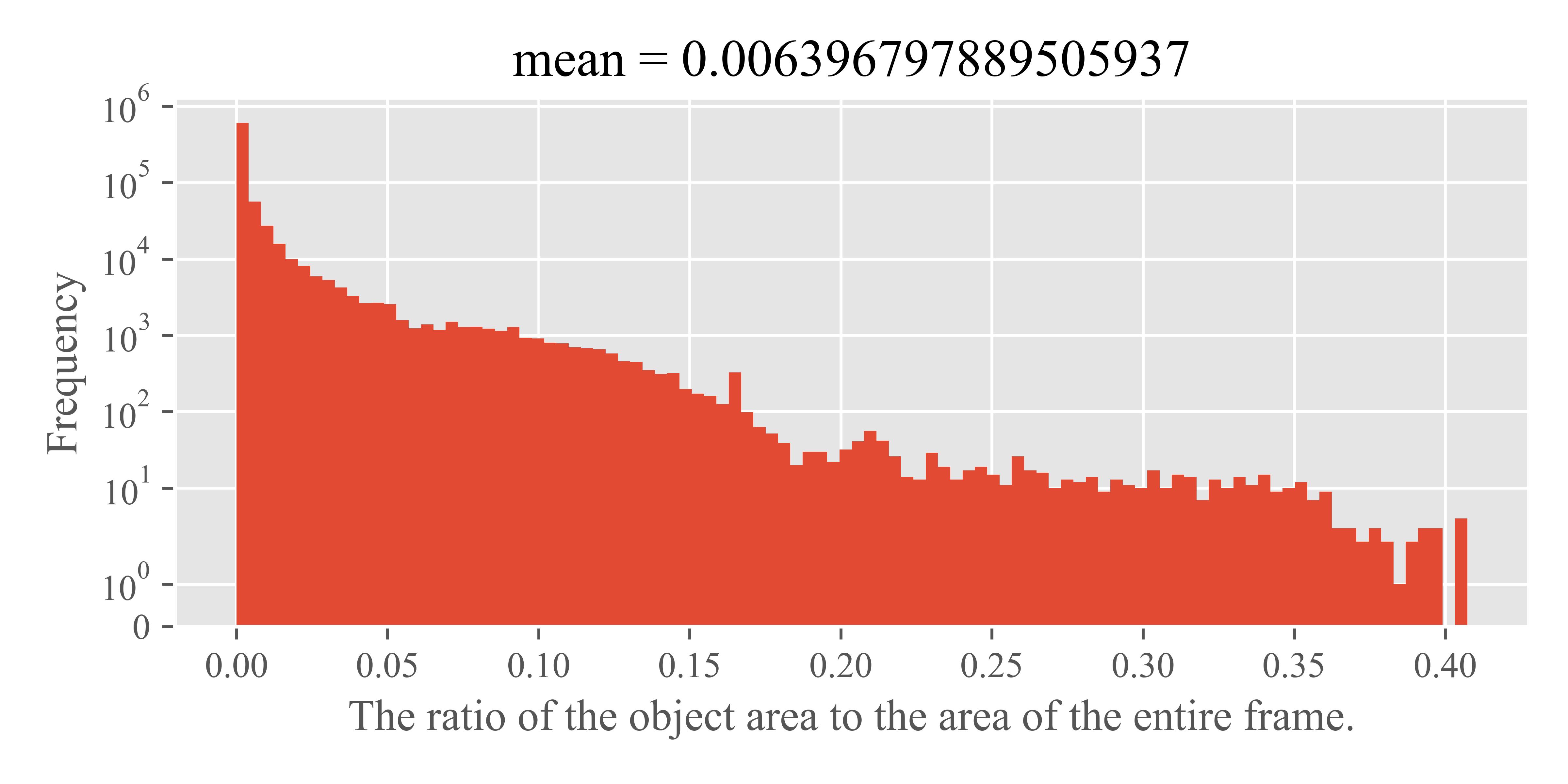
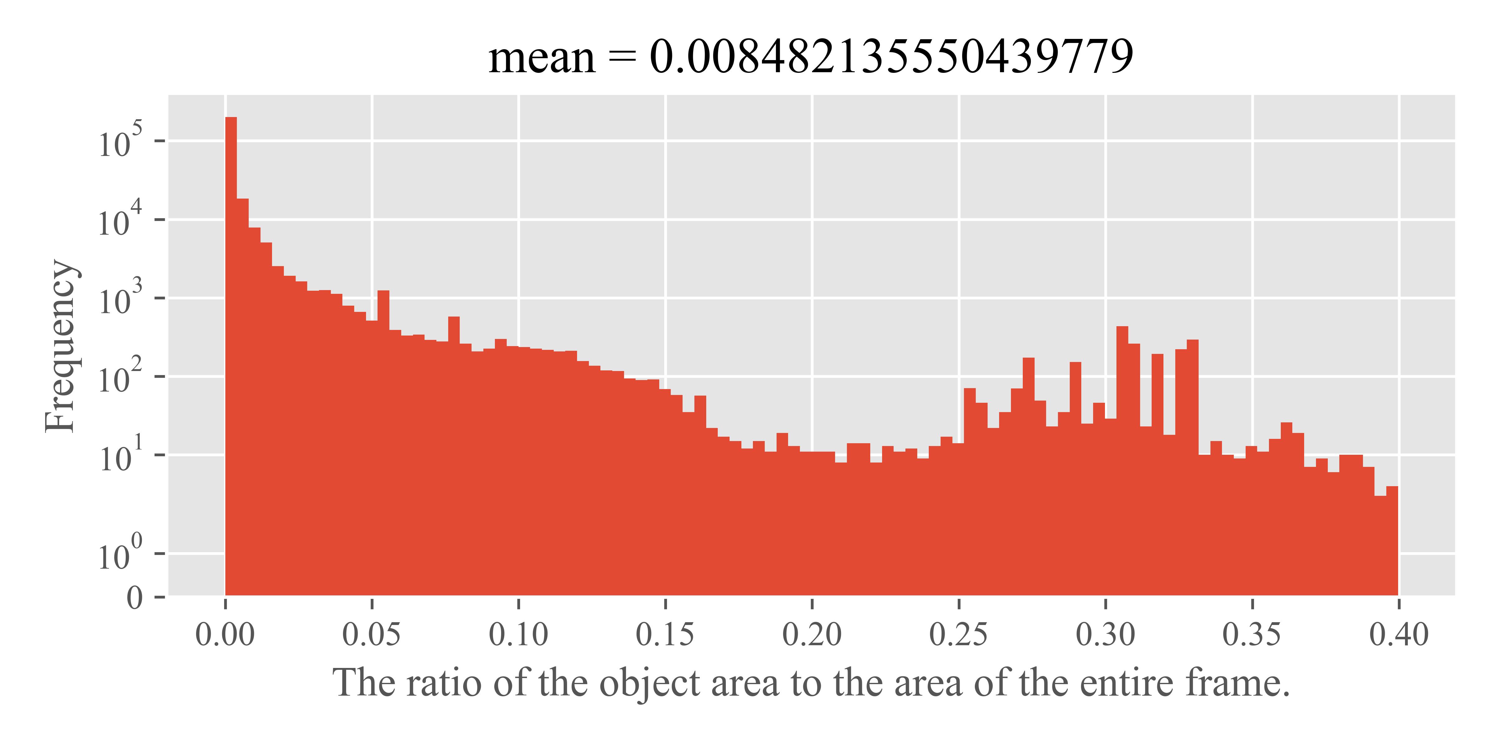
To begin, we analyzed the area ratios of objects in both the training and validation sets of the Argoverse-HD dataset. This involved calculating the ratio of the pixel area covered by an object’s bounding box to the total pixel area of the frame. We visualized these ratios in histograms shown in Fig. 7. The analysis revealed that the mean object area ratio is below 1e-2, indicating a substantial presence of small objects in the dataset. For simplicity in subsequent discussions, we define objects with an area ratio less than 1% as ‘small objects’.
Tab. 12 presents our findings on the proportion of small objects within the Argoverse-HD validation set. Despite some variability in the overall number of objects and small objects, the proportion of small objects remains relatively stable, as reflected in the variance of their proportion. This stability suggests that small objects are a consistent and prominent feature across various video segments, representing a persistent challenge of streaming perception.
| sid | # obj | # small obj | proportion |
| 12 | 27829 | 24033 | 86% |
| 3 | 16557 | 15937 | 96% |
| 14 | 15058 | 14260 | 95% |
| 15 | 12685 | 10229 | 81% |
| 9 | 12618 | 11216 | 89% |
| 5 | 12189 | 9509 | 78% |
| 21 | 11801 | 10259 | 87% |
| 18 | 11073 | 9856 | 89% |
| 20 | 11068 | 10203 | 92% |
| 7 | 10962 | 9707 | 89% |
| 23 | 10961 | 9839 | 90% |
| 2 | 10717 | 9700 | 91% |
| 10 | 10706 | 9001 | 84% |
| 22 | 10122 | 8846 | 87% |
| 11 | 9965 | 8976 | 90% |
| 4 | 9180 | 7989 | 87% |
| 1 | 9068 | 8153 | 90% |
| 24 | 8293 | 7830 | 94% |
| 19 | 8068 | 6552 | 81% |
| 17 | 4709 | 4230 | 90% |
| 6 | 4420 | 3708 | 84% |
| 16 | 7001 | 6508 | 93% |
| 13 | 5654 | 5251 | 93% |
| 8 | 3237 | 2449 | 76% |
| mean | 10580 | 9343 | 87.96% |
| var | – | – | 0.0026 |
A.4 Impact of Environmental Speed
In Sec. A.3, we highlighted how motion within the observer’s viewpoint can affect the perception of small objects. This observation leads us to consider that the speed of the environment could interact with the proportion of small objects.
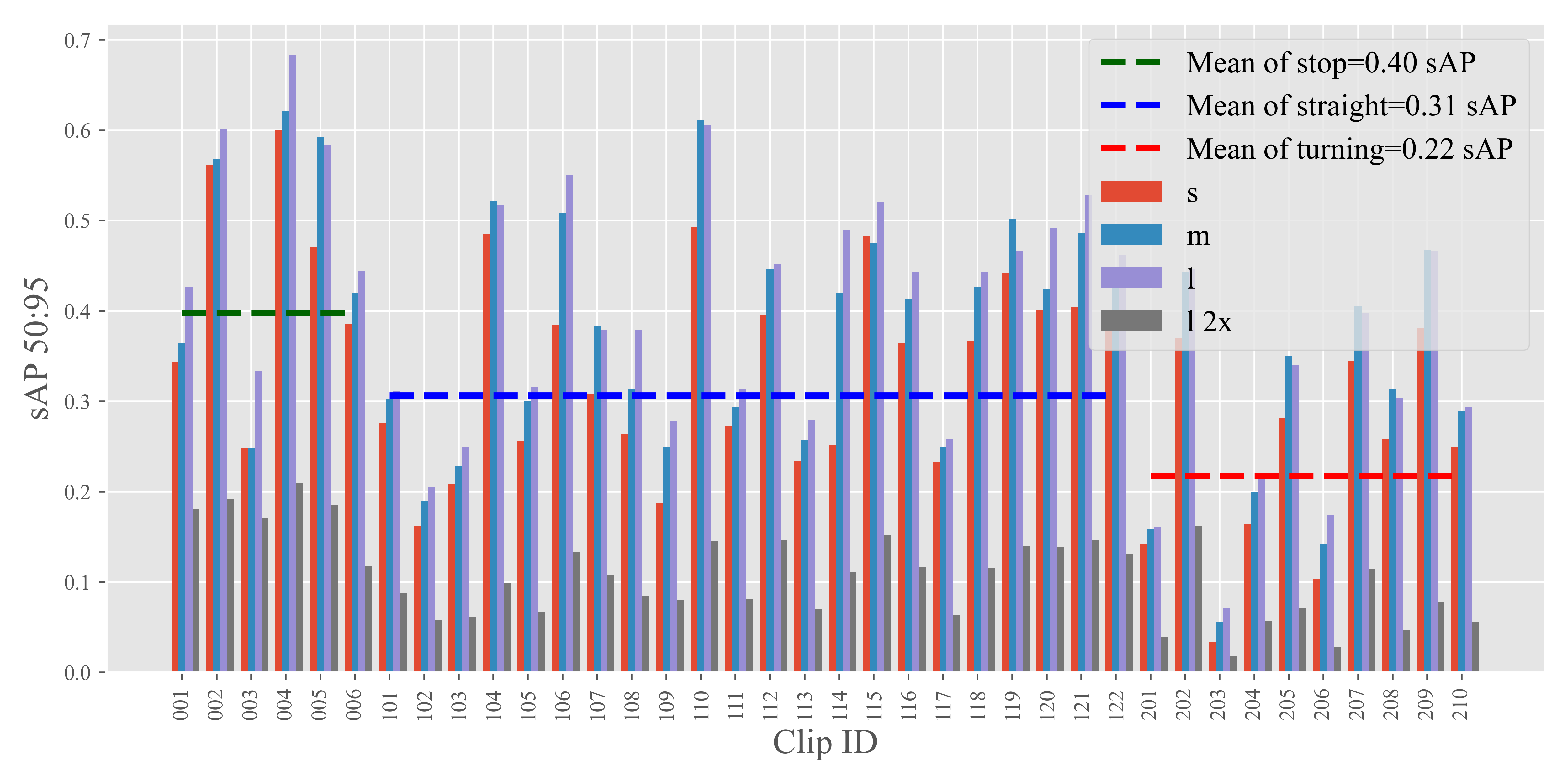
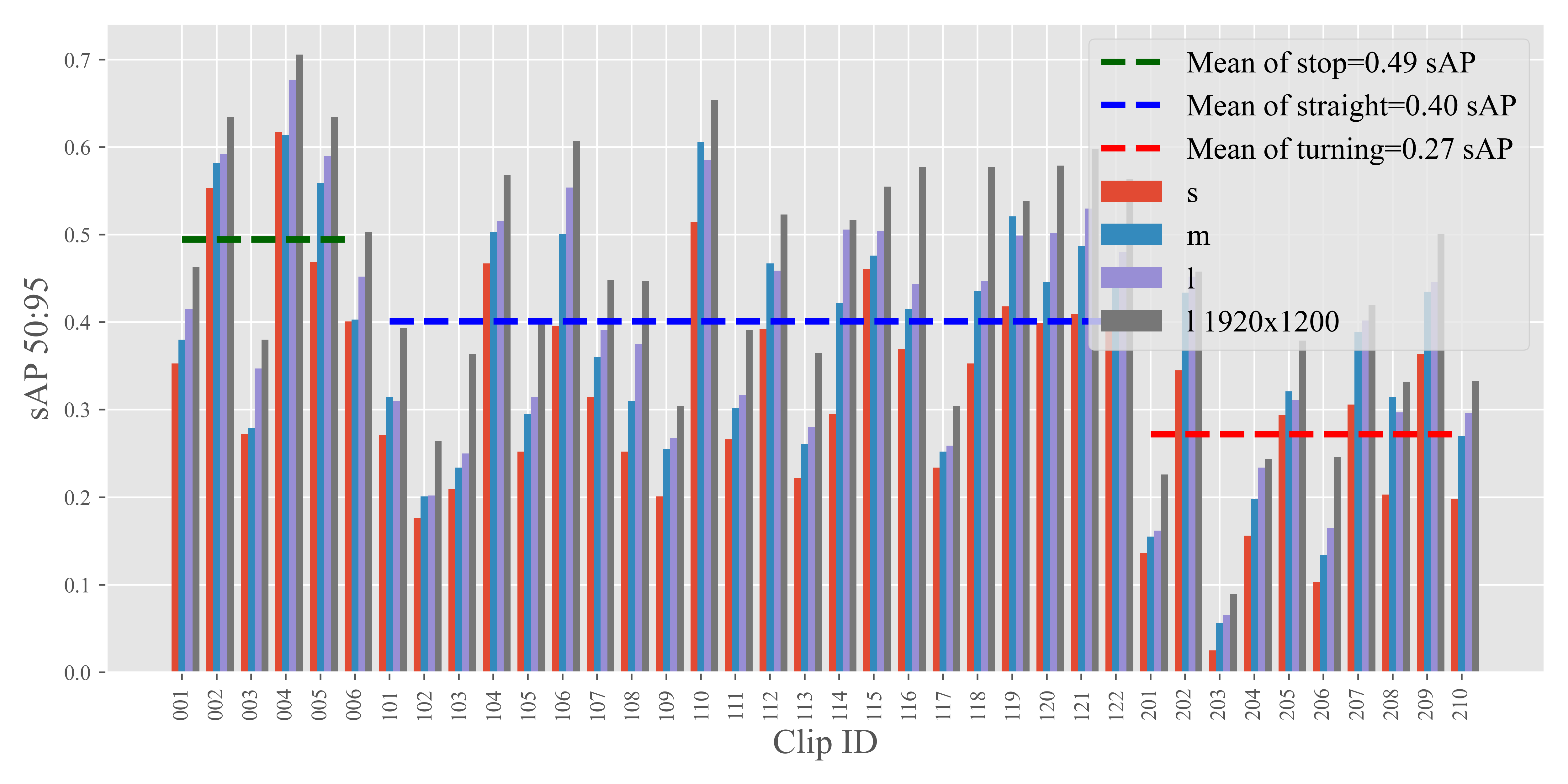
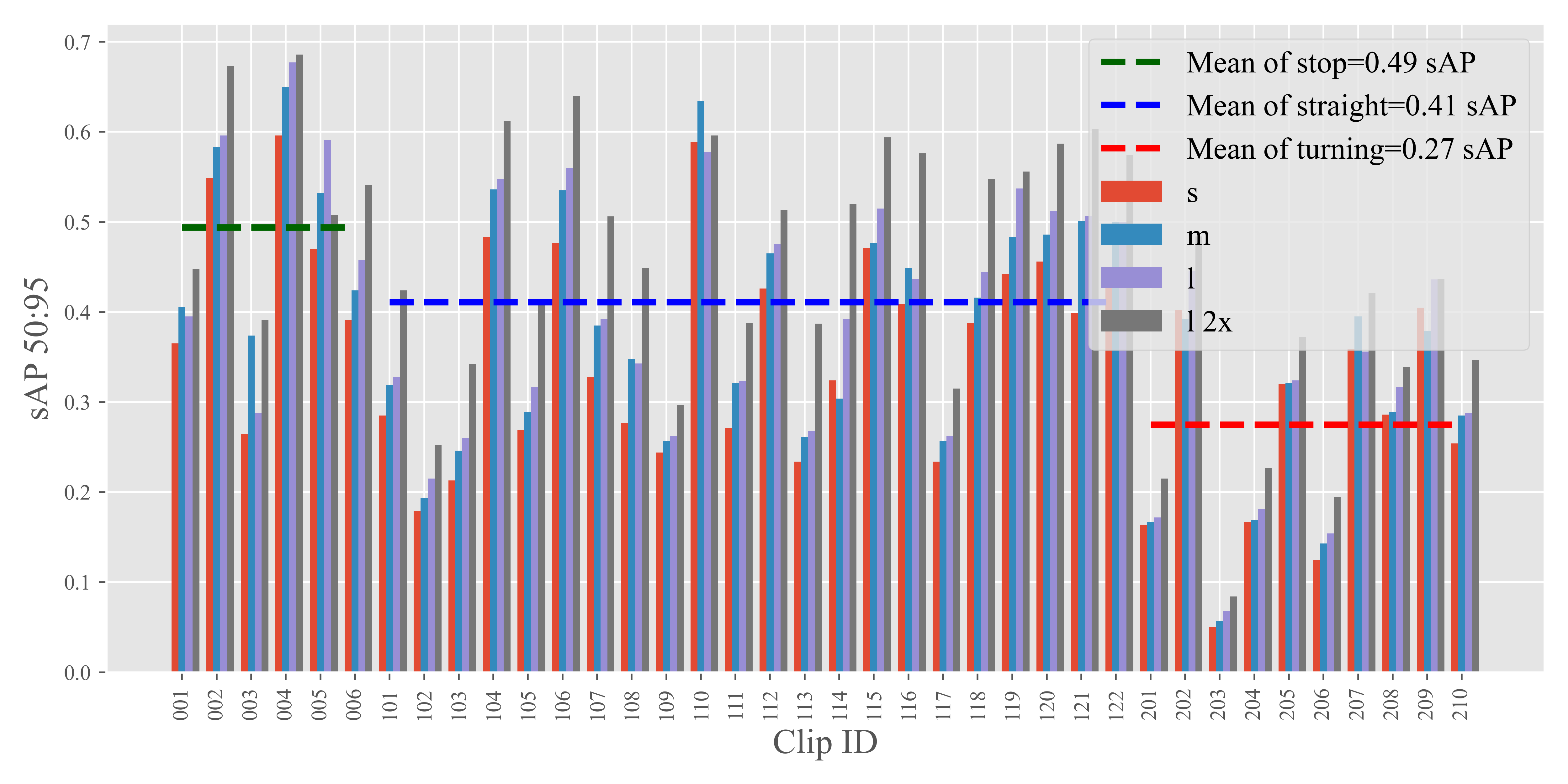
To investigate the relationship between the environmental speed and the performance variability of streaming perception models, we categorized the validation dataset into three distinct environmental states: stop, straight, and turning. We then manually divided the dataset based on these states. In this reorganized dataset, the clips with an ID’s first digit as 0 exclusively represent the stop state, while the digits 1 and 2 correspond to straight and turning states, respectively.
Fig. 8 showcases the performance of StreamYOLO, LongShortNet, and DAMO-StreamNet across each of these segments. Additionally, the mean performance under each motion state is calculated and presented. The data reveals a consistent pattern across all three models: the performance ranking in different environmental motion states follows the order of stop being better than straight, which in turn is better than turning. This trend indicates an association between the state of environmental motion and fluctuations.
Consequently, based on this analysis, we infer that the speed of the environment, particularly when considering the substantial proportion of small objects and their sensitivity to environmental dynamics, emerges as the most influential environmental factor in the context of streaming perception.
Appendix B More Experiment Results
B.1 Inference Time Analysis
This subsection supplements Section 4.4 of the main paper, where we previously discussed the performance of DyRoNet but did not extensively delve into its inference time characteristics. To address this, Tab. 13 presents a detailed comparison of the inference times for each independent branch used in our model. It is important to note that the inference times reported here may show variations when compared to those published by the original authors of the models. This discrepancy is primarily due to differences in the hardware platforms used and the specific configurations of the corresponding models in our experiments.
An interesting observation from the results is that there are instances where DyRoNet exhibits a slower inference time compared to either the random selection method or branch 1. This slowdown is attributed to the incorporation of the speed router in our sample routing mechanism. Despite this, it is evident from the overall results that DyRoNet, employing the router strategy, still retains real-time processing capabilities across the various branches in the model bank. Moreover, in certain scenarios, DyRoNet demonstrates even faster inference speeds than when using individual branches independently. This detailed analysis underlines the dynamic and adaptive nature of DyRoNet in balancing between inference speed and accuracy, highlighting its capability to optimize streaming perception tasks in real-time scenarios.
| Branches | branch 0 | branch 1 | random | DyRoNet |
|---|---|---|---|---|
| 29.26 | 33.65 | 36.61 | 33.22 | |
| 29.26 | 36.63 | 35.12 | 39.60 | |
| 33.65 | 36.63 | 37.30 | 37.61 | |
| 22.08 | 25.88 | 24.79 | 21.47 | |
| 22.08 | 31.24 | 21.49 | 30.48 | |
| 25.88 | 31.24 | 24.75 | 29.05 | |
| 18.76 | 23.01 | 39.16 | 26.25 | |
| 18.76 | 27.85 | 24.04 | 29.35 | |
| 23.01 | 27.85 | 24.69 | 23.51 |
B.2 Statistic of model selection
We also provide statistics on DyRoNet’s selection of different models during both training and inference time in Tab.14. From the results, it can be observed that DAMO-StreamNet (M+L) exhibits a bias to select the second model during inference time, leading to a similar performance as DAMO-StreamNet L. However, under normal circumstances, DyRoNet can still dynamically choose the appropriate model based on input conditions.
| Model | training time | inference time | ||
|---|---|---|---|---|
| Combination | Model 1 | Model 2 | Model 1 | Model 2 |
| SYOLO S+M | 14.24% | 85.76% | 5.95% | 94.05% |
| SYOLO S+L | 10.98% | 89.02% | 4.83% | 95.17% |
| SYOLO M+L | 37.53% | 62.47% | 94.67% | 5.33% |
| LSN S+M | 13.05% | 86.95% | 81.65% | 18.35% |
| LSN S+L | 7.28% | 92.72% | 17.26% | 82.74% |
| LSN M+L | 30.86% | 69.14% | 19.87% | 80.13% |
| DAMO S+M | 6.26% | 93.74% | 0.00% | 100.00% |
| DAMO S+L | 35.29% | 64.71% | 3.69% | 96.31% |
| DAMO M+L | 84.61% | 15.39% | 0.02% | 99.98% |
B.3 The comparison between Speed Router and
| Model Bank | (sAP) | Speed Router (sAP) |
|---|---|---|
| 31.5 | 32.6 (+1.1) | |
| 32.9 | 35.0 (+2.1) | |
| 34.2 | 34.6 (+0.4) |
We also consider a special case id Tab.15, where the model selection only base on the mean of without using Speed Router, which is denoted as . To be specific, the larger model is selected when and minor model is selected otherwise. Unlike Tab.5 in the main text, both methods here are trained for 5 epoch using LoRA fine-tuning. From the results in Tab.15, it can be seen that our proposed Speed Router has significant advantages compared to directly using to select branches.
| train | 0.24% | 48.22% | 51.55% |
|---|---|---|---|
| test | 0.30% | 49.85% | 49.85% |
| val | 0.17% | 49.18% | 50.66% |
Furthermore, in Tab.16, we also conducted the statistic the sign of on the Argoverse-HD. Results with absolute values less than 1e-6 were considered equal to 0. The results reveal that evenly distributing training across models did not effectively adapt them to varying speeds as our Speed Router did.
Appendix C More Details of DyRoNet
| Model | Scale | # of params |
|---|---|---|
| StreamYOLO | S | 9,137,319 |
| M | 25,717,863 | |
| L | 54,914,343 | |
| LongShortNet | S | 9,282,103 |
| M | 25,847,783 | |
| L | 55,376,515 | |
| DAMO-StreamNet | S | 18,656,357 |
| M | 50,129,333 | |
| L | 94,156,945 |
C.1 Pre-trained Model Selection
As outlined in the main paper, our implementation of DyRoNet incorporates three existing models as branches within the Model Bank : StreamYOLO[35], LongShortNet[19], and DAMO-StreamNet[10]. These models were selected due to their specialized features and proven effectiveness in streaming perception tasks. StreamYOLO is unique for its two additional pre-trained weight variants, each tailored for different streaming processing speeds. This feature allows for adaptable performance depending on the speed requirements of the streaming task. In contrast, LongShortNet and DAMO-StreamNet are equipped with pre-trained weights optimized for high-resolution image processing, making them suitable for scenarios where image clarity is paramount.
To ensure a diverse and versatile range of options within the Model Bank, our implementation of DyRoNet selectively utilizes the Small (S), Medium (M), and Large (L) variants of the pre-trained weights from each model. This choice enables a balanced mix of processing speeds and resolution handling capabilities, catering to a wide range of streaming perception scenarios. The specific details regarding the number of parameters for these pre-trained models can be found in Tab.17, which provides a comparative overview to help in understanding the computational complexity for different tasks.
C.2 Setting of Hyperparameters
For all our experiments, we maintained consistent training hyperparameters to ensure comparability and reproducibility of results. The experiments were executed on four RTX 3090 GPUs. Considering the need for selecting the optimal branch model for each sample during the routing process, we established a batch size of , effectively allocating one sample to each GPU for parallel computation.
In alignment with the configuration used in StreamYOLO, we employed Stochastic Gradient Descent (SGD) as our optimization technique. The learning rate was set to , adapting to the batch size proportionally. Additionally, we incorporated a cosine annealing schedule for the learning rate, integrated with a warm-up phase lasting one epoch to stabilize the initial training process.
Regarding data preprocessing, we ensured uniformity by resizing all input frames to pixels. This standardization was crucial for maintaining consistency across different datasets and ensuring that our model could generalize well across various input dimensions.
Appendix D Details of experiment on NuScenes-H dataset
To meet the requirements of streaming perception tasks, nuScenes-H [30] enhances the commonly used autonomous driving perception dataset nuScenes [2] by increasing the annotation frequency from 2Hz to 12Hz. While nuScenes encompasses data from three modalities—Camera, LiDAR, and Radar—nuScenes-H provides dense 3D object annotations exclusively for the 6 sensors of Camera modality.
As mentioned in the main text, we trained and evaluated DyRoNet on the nuScenes-H dataset. To accommodate the requirements for 2D object detection, the 3D object annotations in nuScenes-H are converted to 2D using publicly available conversion scripts. All experiments were conducted exclusively using the CAM_FRONT viewpoint. The dataset partition details are summarized in Tab. 18, which includes the number of video clips, video frames, and the instance counts for each object category within the subsets. As it shows in Tab. 18, limited or even absent annotation for some categories resulted in lower overall test performance. For clarity, this dataset is referred to as nuScenes-H 2D as follows.
Before training DyRoNet, YOLOX [6] was trained for 80 epochs on nuScenes-H 2D to obtain pretrained weights. These weights were then used to initialize the branch models within DyRoNet. During the training of DyRoNet, each individual branch was trained for 10 epochs, followed by 5 epochs of training for the router. All other training settings were consistent with those described in the main text. As indicated by the experimental results presented, DyRoNet maintains strong selection capabilities across different branches on other datasets, demonstrating its adaptability under practical application conditions.
| train set | test set | |
|---|---|---|
| # of video clips | 120 | 30 |
| # of frames | 26705 | 6697 |
| # of anno | 225346 | 71819 |
| adult | 32200 | 13920 |
| child | 22 | 142 |
| wheelchair | 0 | 0 |
| stroller | 0 | 174 |
| personal_mobility | 0 | 2 |
| police_officer | 0 | 0 |
| construction_worker | 1573 | 362 |
| animal | 22 | 0 |
| car | 100487 | 25356 |
| motorcycle | 4958 | 330 |
| bicycle | 1844 | 1248 |
| bus.bendy | 531 | 283 |
| bus.rigid | 4854 | 1161 |
| truck | 21801 | 4934 |
| construction | 2154 | 1200 |
| emergency.ambulance | 61 | 0 |
| emergency.police | 112 | 0 |
| trailer | 6799 | 805 |
| barrier | 33058 | 10568 |
| trafficcone | 8654 | 10096 |
| pushable_pullable | 5191 | 649 |
| debris | 666 | 348 |
| bicycle_rack | 359 | 241 |