Dynamics of the $O(4)$ critical point in QCD: critical pions and diffusion in Model G

The theory we are considering is a generalization of “Model G” of [2] and was first introduced in [3]. It is the relevant hydrodynamic theory constructed around the $O(4)$ critical point of “2-flavor chiral QCD”, namely QCD with massless up and down quarks ($m_{u}=m_{d}=0$). It contains a $O(4)$ order parameter $\phi_{a}\equiv(\sigma,\vec{\pi})$, a proxy for the quark condensate of real QCD, dynamically coupled to vector and axial charges³³3 Here $a$ and $b$ denote $O(4)$ indices; $s$, $s_{1}$, $s_{2}$, etc. denote the three isospin indices, i.e. the components of $\vec{\pi}=(\pi_{1},\pi_{2},\pi_{3})$; finally, spatial indices are notated $i$, $j$ and $k$. The dot product indicates an appropriate contraction of indices when clear from context, e.g. $\phi\cdot\phi=\phi_{a}\phi_{a}$, $\vec{\pi}\cdot\vec{\pi}=\pi_{s}\pi_{s}$, and $\nabla\cdot\nabla=\partial_{i}\partial^{i}$. , $n_{V}^{s}$ and $n_{A}^{s}$ respectively. They correspond to the original iso-vector and iso-axial vector currents, $\vec{n}_{V}\sim\bar{q}\gamma^{0}\vec{t}_{I}q$ and $\vec{n}_{A}\sim\bar{q}\gamma^{0}\gamma^{5}\vec{t}_{I}q$, respectively. These can be conveniently combined into an antisymmetric tensor of charge densities $n_{ab}\in\mathfrak{o}(4)$:

	$\displaystyle(n_{V})_{s}$	$\displaystyle=\frac{1}{2}\epsilon_{0ss_{1}s_{2}}n_{s_{1}s_{2}}\,,$		(1)
	$\displaystyle(n_{A})_{s}$	$\displaystyle=n_{0s}\,.$		(2)

The free energy (or effective Hamiltonian) in the presence of an explicit symmetry breaking $H_{a}=(H,\vec{0})$ can be studied using an $O(4)$ Landau-Ginzburg action

$$\mathcal{H}\equiv\int d^{3}x\left[\frac{n^{2}}{4\chi_{0}}+\frac{1}{2}\partial_{i}\phi_{a}\partial^{i}\phi_{a}+V(\phi)-H\cdot\phi\right]\,,$$

(3)

where

$$V(\phi)=\frac{1}{2}m_{0}^{2}\,\phi^{2}+\frac{\lambda}{4}(\phi\cdot\phi)^{2}\,,$$

(4)

with $m_{0}^{2}$ negative. In equilibrium, the charges have Gaussian fluctuations set by a susceptibility $\chi_{0}$, which is the same coefficient for both the iso-vector and the iso-axial-vector charges near the critical point. The interactions between the charges and the order parameter enters the dynamics through the equations of motion and are determined by the non-trivial Poisson brackets between these fields – see [3, 27] for explicit expressions and a derivation. This construction leads to the following evolution equations

	$\displaystyle\partial_{t}\phi_{a}+\frac{g}{\chi_{0}}\,n_{ab}\phi_{b}$	$\displaystyle=-\Gamma_{0}\frac{\delta\mathcal{H}}{\delta\phi_{a}}+\theta_{a}\,,$		(5a)
		$\displaystyle=\Gamma_{0}\nabla^{2}\phi_{a}-\Gamma_{0}(m_{0}^{2}+\lambda\phi^{2})\phi_{a}+\Gamma_{0}H_{a}+\theta_{a}\,,$		(5b)
	$\displaystyle\partial_{t}n_{ab}+g\,\nabla\cdot(\nabla\phi_{[a}\phi_{b]})+H_{[a}\phi_{b]}$	$\displaystyle=\sigma_{0}\nabla^{2}\frac{\delta\mathcal{H}}{\delta n_{ab}}+\partial_{i}\Xi_{ab}^{i}\,,$		(5c)
		$\displaystyle=D_{0}\nabla^{2}n_{ab}+\partial_{i}\Xi_{ab}^{i}\,.$		(5d)

Here, for example, $H_{[a}\phi_{b]}$ denotes the anti-symmetrization, $H_{a}\phi_{b}-H_{b}\phi_{a}$. The coefficients $\Gamma_{0}$ and $\sigma_{0}$ are the bare kinetic coefficients associated with the order parameter and the charges. The bare diffusion coefficient of the charges is $D_{0}=\sigma_{0}/\chi_{0}$. The constant $g$ is a coupling of the field $\phi$, and has the units of $({\rm action})^{-1}$ in our conventions. Finally, $\theta_{a}$ and $\Xi_{ab}$ are the appropriate noises, which are defined through their two-point correlations [2]

	$\displaystyle\langle\theta_{a}(t,x)\theta_{b}(t^{\prime},x^{\prime})\rangle$	$\displaystyle=2T_{c}\Gamma_{0}\,\delta_{ab}\,\delta(t-t^{\prime})\delta^{3}(x-x^{\prime})\,,$		(6a)
	$\displaystyle\langle\Xi^{i}_{ab}(t,x)\Xi^{j}_{cd}(t^{\prime},x^{\prime})\rangle$	$\displaystyle=2T_{c}\sigma_{0}\,\delta^{ij}\left(\delta_{ac}\delta_{bd}-\delta_{ad}\delta_{bc}\right)\,\delta(t-t^{\prime})\delta^{3}(x-x^{\prime})\ .$		(6b)

The dissipative Model G dynamics relaxes to the equilibrium distribution for the fields $\phi_{a}$ and $n_{ab}$ [2]

$$P[\phi,n]=\frac{1}{Z}e^{-\mathcal{H}[\phi,n]/T_{c}}\,,$$

(7)

which reproduces the static critical behavior of the $O(4)$ model.

The basic observable that will be analyzed are statistical two-point function between fields as a function of relative momentum and time. In the presence of the explicit breaking $H_{a}=H\delta_{a0}$ the flavor index can always be decomposed in a longitudinal $\sigma$ and transverse $\vec{\pi}$ direction, therefore it is natural to define:

$\displaystyle G_{\sigma\sigma}(t,{\bm{k}})=\frac{1}{V}\langle\phi_{0}(t,{\bm{k}})\phi_{0}(0,-{\bm{k}})\rangle_{c}\,,$

(8)

for the scalar channel, and

$\displaystyle G_{\pi\pi}(t,{\bm{k}})=\frac{1}{3V}\sum_{s=1}^{3}\langle\pi_{s}(t,{\bm{k}})\pi_{s}(0,-{\bm{k}})\rangle_{c}\,,$

(9)

for the pseudo-scalar channel. The statistical correlators for the charges are defined analogously

	$\displaystyle G_{AA}(t,{\bm{k}})$	$\displaystyle=\frac{1}{3V}\sum_{s=1}^{3}\langle n_{As}(t,{\bm{k}})n_{As}(0,-{\bm{k}})\rangle_{c}\,,$		(10)
	$\displaystyle G_{VV}(t,{\bm{k}})$	$\displaystyle=\frac{1}{3V}\sum_{s=1}^{3}\langle n_{Vs}(t,{\bm{k}})n_{Vs}(0,-{\bm{k}})\rangle_{c}\ .$		(11)

Note that all these correlators can be studied in mean field, see [27].

At zero explicit breaking $H=0$, we will also consider isotropized $O(4)$ charge and field correlators

	$\displaystyle G_{\phi\phi}(t,{\bm{k}})$	$\displaystyle=\frac{1}{4V}\sum_{a}\langle\phi_{a}(t,{\bm{k}})\phi_{a}(0,-{\bm{k}})\rangle_{c},$		(12)
	$\displaystyle G_{nn}(t,{\bm{k}})$	$\displaystyle=\frac{1}{6V}\sum_{a>b}\langle n_{ab}(t,{\bm{k}})n_{ab}(0,-{\bm{k}})\rangle_{c}\ .$		(13)

This paper is a continuation of [1] and presents results obtained by numerically solving equations (5a)-(5d), using an algorithm detailed in Appendix A of [1]. The stepper combines a symplectic integrator for the Hamiltonian evolution and Metropolis updates for the dissipative step. Throughout we will present our results in lattice units, setting $g=T_{c}=1$, and setting the lattice spacing to unity, $a=1$. This amounts to setting $\hbar=1$ and $T_{c}=1$ and choosing the microscopic lattice spacing so that the model reproduces the correlation length of the physical system. The pole frequency of the pion near the critical point is reproduced by this choice of units. The quartic coupling is set to $\lambda=4$ and the model is simulated close to its critical mass, $m_{c}^{2}(\lambda)=-4.8110(4)$. The reduced temperature and magnetic field are defined as in [12] :

$$t_{r}\equiv\frac{m_{0}^{2}-m_{c}^{2}}{|m_{c}^{2}|}\,,\qquad h\equiv\frac{H}{H_{0}}\,,$$

(14)

where $H_{0}=5.15(5)$ is chosen so that the magnetization scales as

$$\bar{\sigma}=h^{1/\delta}\,,$$

(15)

on the critical line, $t_{r}=0$. For $H=0$ and in the broken phase the magnetization scales as

$$\bar{\sigma}=B^{-}(-t_{r})^{\beta}\ ,$$

(16)

with amplitude⁴⁴4Note an unfortunate misprint in [1]. Equation (29) in the published version should read $\Sigma=b_{1}(m_{c}^{2}-m^{2})^{\beta}(1+C_{T}(m_{c}^{2}-m^{2})^{\omega\nu})$. The then quoted parameters $b_{1}=0.544\pm 0.004$ and $C_{T}=0.20\pm 0.02$ lead to a parametrization $\bar{\sigma}=B^{-}(-t_{r})^{\beta}(1+B_{1}(-t_{r})^{\nu\omega})$ , with $B^{-}=|m_{c}^{2}|^{\beta}b_{1}=0.988\pm 0.007$ and $B_{1}=C_{T}|m_{c}^{2}|^{\omega\nu}=0.49\pm 0.05$. , $B^{-}=0.988(7)$. The non-universal parameters $B^{-}$ and $H_{0}$ completely fix the properties of the magnetic equation of state close to the critical point.

For the static critical exponents quoted here and below we take the values $\beta=0.380(2)$ and $\delta=4.824(9)$ from  [12]. For the correction-to-scaling exponent we take $\omega=0.755(5)$ [46] and the for the dynamical critical exponent we take $\zeta=d/2$ [3], where $d=3$ is the number of spatial dimensions. A summary of all exponents used in this work is given in Table 2 of App. B.

We performed additional analyses along the critical line using the data generated in [1] for different lattice sizes $L$. We also generated an extensive set of data at $H=0$, both in the broken ($m^{2}_{0}<m_{c}^{2}$) and restored ($m^{2}_{0}>m_{c}^{2}$) phases. The dynamical parameters were chosen as in our previous work, $\chi_{0}=5$, $\Gamma_{0}=1$ and $D_{0}=1/3$. Our full dataset is summarized in Table 1.

For context, we also display the correlation length (in lattice units) for our different simulations in Fig. 1. The correlation lengths in the restored phase and on the critical line correspond to the fits presented in App. B.1 and B.2. As discussed below, in the broken phase the hydrodynamic theory is characterized by a pion EFT at the longest wavelengths. The pion parameter $f^{2}(T)$ is a matching coefficient in the EFT, which characterizes the pion’s fluctuations and scales as the inverse correlation length close to the critical point [47, 5]. We will use $1/{(2f^{2})}$ as an estimate for the correlation length in the broken phase which is determined numerically in App. B.3. Here the factor of $\tfrac{1}{2}$ is conventional and is motivated by the fact that finite volume corrections to correlation functions (which are computable using the pion EFT [47]) are organized in powers of $1/(2f^{2}L)$ with order one coefficients, see App. B.3. The black data points correspond to the different temperatures we simulated.

Before diving into a quantitative study, we use the rest of this section to present the qualitative behavior of the different channels in the restored and broken phases (with $H=0$) and on the critical line ($t_{r}=0$ and $H\neq 0$).

In the restored phase, the $O(4)$ symmetry is unbroken and there is no distinction between the axial and vector channels. The order parameter simply dissipates towards equilibrium on a finite (if long) timescale. But, both the iso-vector and iso-axial vector charges are exactly conserved. As a result, the non-trivial dynamics at the longest wavelengths is fully encoded in the correlators of conserved charges at finite momenta. Indeed, for wavelengths long compared to the (diverging) correlation length $k\xi(T)\ll 1$, the diffusion equation remains a valid hydrodynamic description of the system:

$$\partial_{t}n_{ab}=D\nabla^{2}n_{ab}\,.$$

(17)

Thus, the relaxation rate of a diffusive mode of wavenumber $k$ is controlled by the diffusion coefficient $Dk^{2}$ leading to the correlators (see App. A.1):

$$G_{AA}(t,{\bm{k}})=G_{VV}(t,{\bm{k}})=T\chi_{0}e^{-Dk^{2}t}\,.$$

(18)

The charge correlations in the simulation are illustrated on the left-hand side of Fig.2, where we plot the axial correlator (orange) and the vector correlator (blue), for the first two momenta, for a given temperature. We clearly see that the two channels are degenerate. The $k$ dependence is consistent with the expected diffusive behavior.

In writing the diffusion equation in eq. (17) we have integrated out the contributions to the currents from the order parameter, which then leads the scaling behavior of the transport coefficient. As discussed below, the order parameter has a dynamical relaxation time of order $\tau\propto\xi^{\zeta}$ with $\zeta=d/2$. The diffusive modes have a relaxation time of $1/Dk^{2}$, which is of order $\xi^{2}/D$ at the boundary of applicability of the diffusion equation, $k\sim\xi^{-1}$. In the spirit universality, all modes of with wavelengths of order $\xi$ should have a similar relaxation time, dictating the expected scaling of the diffusion coefficient, $D\propto\xi^{2-\zeta}$.

On the right-hand side of Fig. 2, we show the dependence of the vector correlator (we could have equivalently chosen the axial) on $t_{r}$. This very weak dependence seems at first to be in contradiction with the expected critical scaling of the diffusion coefficient $D\sim t_{r}^{(\zeta-2)\nu}$. As we will see more clearly in the next section, this apparent contradiction originates in the presence of a large regular constant contribution to $D$, and by the smallness of its non-universal critical amplitude. Nevertheless, we will extract the critical contribution to $D$ in Sect. III.1.

We next study the critical line, $m^{2}_{0}=m_{c}^{2}$, and study the effect of explicit symmetry breaking, $H\neq 0$. One of the qualitative outcomes of our previous work [1] was to demonstrate the emergence of damped pion waves already on the critical line. This qualitative observation was obtained from the $k=0$ modes of the axial current and the pions correlators. The same qualitative observation holds for non-zero momentum $k$ and is observed in Fig. 3. At the level of the charge correlators, the magnetic field lifts the degeneracy between the axial and vector channels. The axial correlator then displays characteristic oscillations associated with axial charge propagation in the form of damped pion waves. The vector channel on the other hand remains purely diffusive. As in the restored phase, we already observe that the critical behavior of the vector diffusion constant is weak.

Below the critical point the longest wavelength modes are characterized by massless Goldstone bosons, which describe phase fluctuations of the chiral condensate⁵⁵5For clarity we will restore the temperature in this section.. Following [5, 6], these fluctuations are parametrized by an angle $\vec{\varphi}(t,{\bm{x}})$ with $\phi_{a}=(\bar{\sigma},\bar{\sigma}\vec{\varphi}(t,{\bm{x}}))$. We are assuming that the chiral condensate is nearly aligned with the pole of the three sphere (the coset manifold) and takes the form

$$\frac{1}{V}\int_{{\bm{x}}}d^{3}x\,\phi_{a}(t,{\bm{x}})=\bar{\sigma}\,n_{a}\,,$$

(19)

where $n_{a}$ is a unit vector that is approximately parametrized by $n_{a}\simeq(1,\vec{\varphi}_{0})$ to first order in the angular deviation. When the wavelength of $\varphi$ is long compared to the correlation length $\xi\equiv m_{\sigma}^{-1}$, a hydrodynamic description of $\varphi$ is valid, and the fluctuations of modes with wavelength order $m_{\sigma}^{-1}$ simply determine the critical behavior of the parameters of the hydrodynamic theory.

The free energy associated with the phase and charge fluctuations in the hydrodynamic approximation is

$$\mathcal{H}[\varphi,n]=\int{\rm d}^{3}x\,\frac{\vec{n}_{V}^{2}}{2\chi_{0}}+\frac{\vec{n}_{A}^{2}}{2\chi_{0}}+\tfrac{1}{2}f^{2}(T)\,\partial_{i}\vec{\varphi}\cdot\partial^{i}\vec{\varphi}+\tfrac{1}{2}f^{2}m^{2}\varphi^{2}\,,$$

(20)

where we have included a mass term, which is relevant only when the magnetic field is non-zero and is determined by the Gell-Mann, Oakes, Renner relation

$$f^{2}m^{2}=H\bar{\sigma}\,.$$

(21)

We will set $H=m=0$ for the remainder of this section. The resulting hydrodynamic equations of motion for the pions and axial charge take the form⁶⁶6 In [26] the dissipative coefficient $\Gamma/f^{2}$ was called $\zeta^{(2)}$. In mean field theory the hydrodynamic parameter $\Gamma$ equals the bare parameter $\Gamma_{0}$ [27]. A notable feature of these equations when the symmetry is explicitly broken is that the same coefficient $\Gamma/f^{2}$ controls both the damping rate at finite momentum and the mass term, see eq. (65). This is a general result dictated by entropy considerations [3, 26, 48] and related locality arguments [49]. This became widely recognized through a sequence of explicit holographic computations in different contexts with explicitly broken symmetries [50, 51, 52, 53] – for a review see [54]. The pion dynamics in a holographic model of the phase transition is described in [43] and can be profitably compared to mean field theory results of [27].

	$\displaystyle\partial_{t}\vec{\varphi}-\frac{\vec{n}_{A}}{\chi}=$	$\displaystyle\frac{\Gamma}{f^{2}}\,\nabla\cdot(f^{2}\nabla\vec{\varphi})\,,$		(22a)
	$\displaystyle\partial_{t}\vec{n}_{A}-\nabla(f^{2}\nabla\vec{\varphi})=$	$\displaystyle D\nabla^{2}\vec{n}_{A}\,,$		(22b)
which reflects from the Poisson bracket between the phase and the charge, $\{\varphi_{s},n_{As^{\prime}}\}=\delta_{ss^{\prime}}$. The vector charge remains diffusive
	$$\partial_{t}\vec{n}_{V}=D\nabla^{2}\vec{n}_{V}\,.$$			(22c)

The hydrodynamic system is solved in App. A.1 and the resulting pion eigen-waves have dispersion relations

$$\omega(k)-\frac{i}{2}\Gamma(k)=\pm vk-\frac{i}{2}D_{A}k^{2}\,,$$

(23)

where

$$v^{2}\equiv\frac{f^{2}}{\chi_{0}}\quad\mbox{and}\quad D_{A}\equiv\Gamma+D\,.$$

(24)

The form of the correlation function from the hydrodynamic theory is determined in App. A.1

$$G_{\varphi\varphi}(t,{\bm{k}})=\frac{T}{f^{2}k^{2}}e^{-\frac{1}{2}D_{A}k^{2}t}\left[\cos(vkt)+\frac{1}{2vk}(D-\Gamma)k^{2}\sin(vkt)\right]\,.$$

(25)

At large wavelengths the pion effective theory determines the static and dynamic correlation functions. The static correlation function for $k\ll m_{\sigma}$ can be read off from the free energy in (20) and is singular in the massless limit:

$$G_{\pi\pi}(0,{\bm{k}})=\bar{\sigma}^{2}G_{\varphi\varphi}(0,{\bm{k}})=\bar{\sigma}^{2}\,\frac{T}{f^{2}k^{2}}\,,\qquad k\ll m_{\sigma}\,.$$

(26)

By contrast, the static fluctuations of the $\sigma$ are bounded (if diverging) and determined by the static susceptibility of the $O(4)$ critical point, which scales as

$$G_{\sigma\sigma}(0,{\bm{k}})\propto m_{\sigma}^{\eta-2}\qquad k\ll m_{\sigma}\,.$$

(27)

The $\sigma$ and $\vec{\pi}$ are part of an $O(4)$ multiplet and their correlators must be the same order of magnitude at the boundary of applicability of the pion EFT, $k\sim m_{\sigma}$. Since the vev scales as $\bar{\sigma}^{2}\propto m_{\sigma}^{(d-2+\eta)}$, the pion constant must scale as $f^{2}\propto m_{\sigma}^{(d-2)}$ [47]. We have anticipated this scaling in Fig. 3 where $T/2f^{2}$ (with $T=1$ in our adopted units) served as a definition of the correlation length in the broken phase.

Because of these scalings, the long-wavelength behavior of the static and dynamic correlation functions of $\phi_{a}$ are dominated by the phase fluctuations. Specifically, the static correlation function reads

$\displaystyle G_{\phi\phi}(0,{\bm{k}})=\frac{1}{4}\left(G_{\sigma\sigma}(0,{\bm{k}})+3G_{\pi\pi}(0,{\bm{k}})\right)\simeq\frac{3}{4}\,\bar{\sigma}^{2}\,\frac{T}{f^{2}k^{2}}\,,\qquad k\ll m_{\sigma}\,,$

(28)

up to corrections of order $(k/m_{\sigma})^{2}$. Additional finite volume corrections to this formula are given in App. B.3 and are suppressed by $1/f^{2}L$ [47]. Phase fluctuations also determine the dynamic correlations

$$G_{\phi\phi}(t,{\bm{k}})\simeq\frac{3}{4}\,\bar{\sigma}^{2}G_{\varphi\varphi}(t,{\bm{k}})\,,$$

(29)

and Fig. 4 (Left) exhibits the $\phi\phi$ correlation function, which shows characteristic pion oscillations of (25) become increasingly damped near the critical point. The critical scaling of $v$ and $D_{A}$ are extracted numerically in the next section and are ultimately summarized in Fig. 7.

In a finite volume simulation the orientation of the chiral condensate is not fixed, but diffuses in time due to thermal noise. Indeed, a stochastic variable $\xi_{\varphi}$ with variance

$$\left\langle\xi_{\varphi s}(t,{\bm{x}})\xi_{\varphi s^{\prime}}(t^{\prime},{\bm{x}}^{\prime})\right\rangle=\frac{2T\Gamma}{f^{2}}\delta_{ss^{\prime}}\delta(t-t^{\prime})\delta({\bm{x}}-{\bm{x}}^{\prime})\,,$$

(30)

should be added to (22a). Integrating this equation over the volume shows that the angular zero mode $\vec{\varphi}_{0}(t)\equiv\int_{\bm{x}}\vec{\varphi}(t,{\bm{x}})/V$ has a variance which increases in time

$$2\,\mathfrak{D}\,t=\frac{1}{3}\left\langle\vec{\varphi}_{0}(t)\cdot\vec{\varphi}_{0}(t)\right\rangle=2\left(\frac{T\Gamma}{f^{2}V}\right)t\,.$$

(31)

This result (which is presented in detail in App. A.2) relates the vev diffusion coefficient to the pion kinetic coefficients, $\mathfrak{D}=T\Gamma/f^{2}V$. The diffusion rate decreases with increasing volume and is suppressed relative to the pion damping rate, $\Gamma k^{2}\sim\Gamma/L^{2}$, by one power of length, $T/f^{2}L\propto 1/m_{\sigma}L$. When the magnetic field is non-zero the Fokker-Planck equation describing the motion of the chiral condensate on the three sphere features a rich interplay between Hamiltonian and diffusive dynamics, which is developed in App. A.2.

Turning to the conserved charges, the correlation function of the vector and axial-vector charges in the broken phase are intrinsically different. The axial charge is coupled through in equations of motion to the pions and its correlation function reflects this coupling (see App. A.1)

$$G_{AA}(t,{\bm{k}})=T\chi_{0}e^{-\tfrac{1}{2}D_{A}k^{2}t}\left[\cos(vkt)-\frac{1}{2vk}(D-\Gamma)k^{2}\sin(vkt)\right]\,.$$

(32)

The vector charge continues to obey the diffusion equation with corresponding response functions

$$G_{VV}(t,{\bm{k}})=T\chi_{0}e^{-Dk^{2}t}\,.$$

(33)

Separating the vector and axial vector response in the absence of explicit symmetry breaking is challenging, since the condensate forms in an arbitrary direction. Moreover, because of finite volume, this direction is not completely fixed, but slowly wanders along the coset manifold. This can be addressed in future work. For now we have simply computed the combined correlator $G_{nn}(t,{\bm{k}})$

$$G_{nn}(t,{\bm{k}})=\frac{1}{6}\left[3G_{AA}(t,{\bm{k}})+3G_{VV}(t,{\bm{k}})\right]\,,$$

(34)

which is exhibited in Fig. 4 (Right). The result curves show a mix of exponential decay and oscillating pion waves.

It is striking how the hydrodynamic EFT and the pattern of chiral symmetry break essentially dictates the scaling dynamical response of “Model G” [5, 6]. A summary of the reasoning proves an overview of the next section.

1. (i)

   The characteristic frequency of the pion waves below the critical point is of order $\omega(k)\sim vk$ where $v=\sqrt{f^{2}/\chi_{0}}\propto m_{\sigma}^{(d-2)/2}$. The scaling of the velocity will be extracted from the real time correlations of $\phi$, eq. (25), and from its static behavior, eq. (28), and the results are summarized in Fig. 7 (Right).

2. (ii)

   At the boundary of applicability of the pion EFT $k\sim m_{\sigma}$, the pion frequency is $\omega(k)\sim vk\sim m_{\sigma}^{d/2}$. But, since the pions are part of an $O(4)$ multiplet, the order parameter must inherit this dynamical timescale, $\tau\sim m_{\sigma}^{-d/2}$, setting the dynamical critical exponent of Model G, $\zeta=d/2$. $\tau$ will be extracted in the restored phase, Fig. 5 (Left), and on the critical line, Fig. 6 (Left).

3. (iii)

   Close to the critical point and for $k\lesssim m_{\sigma}$, the real and imaginary parts of $\omega(k)$ should be commensurate if the critical point is characterized by a single time scale. This reasoning dictates the scaling of the pion damping coefficient, $D_{A}\propto m_{\sigma}^{d/2-2}$. The scaling of $D_{A}$ is exhibited in Fig. 7 (Left).

4. (iv)

   Since the axial and vector charges must become degenerate above $T_{c}$, the diffusion coefficient must have the same scaling as $D_{A}$, leading to the scaling, $D\sim m_{\sigma}^{d/2-2}$. The scaling of $D$ is exhibited in the restored phase, Fig. 5 (Right), and on the critical line, Fig. 6 (Right).

Finally, the vev diffusion coefficient $\mathfrak{D}$ is also consistent with these scalings. Taking the scaling of $f^{2}\propto m_{\sigma}^{d-2}$ and $\Gamma\propto m_{\sigma}^{d/2-2}$ we see the angular variance given in (31) grows as

$$2\,\mathfrak{D}\,t\propto\frac{t}{(m_{\sigma}L^{2})^{d/2}}\,.$$

(35)

At the critical point where $m_{\sigma}L\rightarrow 1$, the angular variance increases as

$$2\,\mathfrak{D}\,t\rightarrow\frac{t}{L^{d/2}}\,,$$

(36)

which is again consistent with a universal dynamical critical timescale of $\tau\propto L^{\zeta}$ with a common critical exponent of $\zeta=d/2$.

We first determine the order parameter relaxation time $\tau$ from the two-point function $G_{\phi\phi}(t,{\bm{k}})$. Specifically, we define $\tau$ as the autocorrelation time of $G_{\phi\phi}$ at zero momentum $G_{\phi\phi}(t)\equiv G_{\phi\phi}(t,{\bm{0}})$

$$\tau\equiv\int_{0}^{\infty}\mathrm{d}t\,\frac{G_{\phi\phi}(t)}{G_{\phi\phi}(0)}\ ,$$

(37)

which is motivated by an exponential decay, $G_{\phi\phi}\propto e^{-t/\tau}$ (in practice, we cutoff the integral at some $T_{max}$ and make sure the results are independent of this technicality). Qualitatively, the decorrelation of $G_{\phi\phi}(t)$ is characterized by a single timescale $\tau$ without significant structure.

From scaling, we expect the correlation time to behave as

$$\tau(t_{r})=\tau^{+}t_{r}^{-\nu\zeta}(1+\tau_{1}t^{\nu\omega})\,,$$

(38)

with the critical exponents $\nu$, $\omega$, and $\zeta$ given in Table 2 in App. B. The resulting fit (with the exponents fixed) is shown in Fig. 5 and we find

	$\displaystyle\tau^{+}$	$\displaystyle=1.570\pm 0.037,$		(39)
	$\displaystyle\tau_{1}$	$\displaystyle=-1.49\pm 0.15\ .$		(40)

The growth of $\tau$ near the $T_{c}$ is nicely consistent with $\zeta=d/2$.

The diffusion coefficient $D$ of the $O(4)$ charges is also expected to show dynamical critical scaling, but since the charges are conserved, the coefficient has to be extracted from finite momentum correlators. In particular, we expect the vector correlator in the restored phase to behave as

$$G_{VV}(t,{\bm{k}})=T\chi_{0}e^{-Dk^{2}t}\ ,$$

(41)

as discussed in the previous section. Similar to the order parameter case, we have the relation

$$D\equiv\frac{1}{k^{2}}\left(\int_{0}^{\infty}\mathrm{d}t\,\frac{G_{VV}(t,{\bm{k}})}{G_{VV}(0,\bm{0})}\right)^{-1}\ ,$$

(42)

which we use in practice to extract $D$ from our data. It is important that the correlator be well described by an exponential, which is clearly seen in Fig. 2.

Again, we introduce a cutoff $T_{max}$ and make sure the results are independent of this choice. As discussed above, we expect $Dk^{2}$ to be comparable $1/{\tau}\sim\xi^{\zeta}$ at the boundary of applicability of the diffusive description, $k\lesssim\xi$. This means that the diffusion coefficient should scale with the correlation length as, $D\propto\xi^{2-\zeta}$.

The critical behavior of $D$ appears to be weak and its regular part cannot be neglected. To take this into account, we add a constant $D_{0}$ to our fit

$$D(t_{r})=D^{+}t_{r}^{-\nu(2-\zeta)}(1+D_{1}t_{r}^{\omega\nu})+D_{0}\ .$$

(43)

In an abuse of notation, $D_{0}$ here is the renormalized diffusion coefficient far above $T_{c}$, which we determine independently by running our simulations without the coupling to the order parameter, leading to

$$D_{0}\approx 0.2425(5)\ .$$

(44)

This parameter is different from the bare lattice parameter (also called $D_{0}=1/3$) which controls the Metropolis updates of the charge at the scale of the lattice spacing (see [1] in Appendix A.c for further details). Fixing $D_{0}$ and fitting $D^{+}$ and $D_{1}$ in (43), we get the following determination of the non-universal amplitudes

	$\displaystyle D^{+}$	$\displaystyle=0.0190\pm 0.0013\,,$		(45)
	$\displaystyle D_{1}$	$\displaystyle=-1.7\pm 0.55\ .$		(46)

$D^{+}$ is small as was anticipated based on a one loop calculation using mean field propagators [27].

Using the non-universal amplitude $\xi^{+}$ from the correlation length $\xi\sim\xi^{+}t_{r}^{-\nu}$ determined in App. B.1, we can combine these results into a universal dynamical amplitude ratio

$\displaystyle\mathfrak{Q}_{D}^{+}\equiv\frac{D^{+}\tau^{+}}{\xi^{+2}}=0.148\pm 0.011\ ,$

(47)

which numerically encodes the coupling between the charge diffusion and the order parameter relaxation at criticality. The universal dynamical ratio presented here is new and will prove useful to any future study which realizes the critical dynamics of Model G.

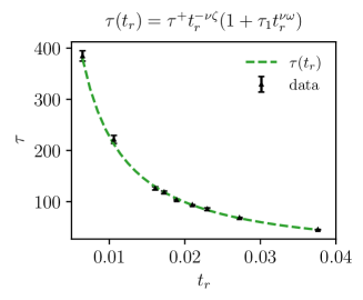
We next study the dynamics on the critical line, $m^{2}_{0}=m_{c}^{2}$ and $H\neq 0$. As in the previous section we define the order parameter relaxation time $\tau$ from the correlation of the $\sigma$ field

$$\tau\equiv\int_{0}^{\infty}\mathrm{d}t\frac{G_{\sigma\sigma}(t,\bm{0})}{G_{\sigma\sigma}(0,\bm{0})}\ .$$

(48)

The results for $\tau$ as a function of the magnetic field are shown in Fig. 6, and are fit with the expected scaling form

$$\tau(H)=\tau^{H}H^{-\nu_{c}\zeta}(1+\tau_{1}H^{\nu_{c}\omega})\ ,$$

(49)

with fixed exponents $\nu_{c}$, $\omega$, and $\zeta$ given in Table 2 of App. B, and fitted parameters

	$\displaystyle\tau^{H}$	$\displaystyle=1.312\pm 0.022\,,$		(50)
	$\displaystyle\tau_{1}^{H}$	$\displaystyle=-1.45\pm 0.06\ .$		(51)

As in the restored phase, the subleading term with exponent $\omega$ is necessary to have a reasonable fit compatible with the expected dynamical exponent, $\zeta=d/2$.

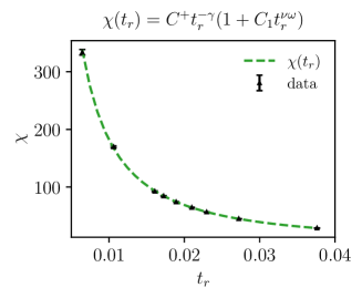
Similarly, the diffusion coefficient is defined in the same way as in the restored phase

$$D\equiv\frac{1}{k^{2}}\left(\int_{0}^{\infty}\mathrm{d}t\,\frac{G_{VV}(t,{\bm{k}})}{G_{VV}(0,{\bm{k}})}\right)^{-1},\text{ with }|{\bm{k}}|=\frac{2\pi}{L},$$

(52)

and we adopt an analogous strategy and functional form to fit the dependence of $D$ on the correlation length

$$D(H)=D^{H}H^{-\nu_{c}(2-\zeta)}(1+D_{1}^{H}H^{\nu_{c}\omega})+D_{0}\,.$$

(53)

As in the previous section, $D_{0}=0.2425$ is the regular part of the diffusion coefficient and is extracted from our diffusion only runs. The fit results are shown in Fig. 6 and the fit parameters are

	$\displaystyle D^{H}$	$\displaystyle=0.023\pm 0.002\,,$		(54)
	$\displaystyle D_{1}^{H}$	$\displaystyle=-1.02\pm 0.42\ .$		(55)

The singular part of the diffusion coefficient diverges next to the critical point with the expected exponent $H^{-\nu_{c}(2-\zeta)}$ and the subleading correction improves the quality of the fit. Including the regular part of the diffusion coefficient $D_{0}$ is crucial to extracting the scaling of $D$ with $H$, since the critical amplitude $D^{H}$ is small, as anticipated in the one loop computation in [27].

The results for the order parameter and the diffusion coefficient can be concisely recast as a universal amplitude ratio

$\displaystyle\mathfrak{Q}_{D}^{H}\equiv\frac{D^{H}\tau^{H}}{\xi^{H2}_{L}}=0.151\pm 0.022\,,$

(56)

where $\xi_{L}^{H}$ is the amplitude associated with the longitudinal correlation length and is determined in App. B.2. Note that within numerical errors the dynamical ratio on the critical line matches the one in the restored phase (47).

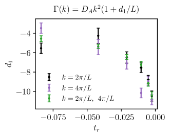
Our aim in this section is to extract the matching coefficients of the pion hydrodynamic EFT by studying the momentum dependence of the correlators and analyzing the pion dispersion curve. To this end, we study $G_{\phi\phi}$ for various $t_{r}$ and $L$ and analyze the two lowest non-zero momentum modes, $k=2\pi/L$ and $k=4\pi/L$. We then perform some fits using the hydro prediction (25) and extract the parameters $\omega(k)$ and $\Gamma(k)$. $\omega(k)$ and $\Gamma(k)$ are subsequently extrapolated to infinite volume using the forms

	$\displaystyle\Gamma(k)$	$\displaystyle=D_{A}k^{2}(1+d_{1}/L),$		(57a)
	$\displaystyle\omega(k)$	$\displaystyle=vk+v_{2}k^{2}\ ,$		(57b)

with $D_{A}$, $v$, $d_{1}$, and $v_{2}$ as parameters. As discussed in Sect. II.5, finite volume corrections to the dynamics of the Goldstone modes scale inversely with the linear extent of the lattice $\sim 1/f^{2}L$ and are therefore important to control. Including $d_{1}$ and $v_{1}$ as fit parameters captures this characteristic volume dependence and proved crucial to reliably extracting $D_{A}$ and $v$ from this analysis. The fitting procedure, together with other systematic checks, are presented in detail in App. C.

In the static case, a finite volume pion EFT was developed many years ago by Hasenfratz and Leutwyler and can be used to determine the first $1/f^{2}L$ correction to the chiral condensate analytically [47]. We used their expansion in App. B.3 to determine velocity $v^{2}=f^{2}/\chi_{0}$ and, as we show below, the result agrees with the dynamic fit using (57). In Sect. II.5 we have taken the first steps in developing a real time finite volume analog of their work by deriving the vev diffusion coefficient in (31) and a corresponding forced Fokker-Planck equation on the coset manifold in App. A.2. But, a more complete analysis is left for future work.

Knowing $v$ and $D_{A}$, we can proceed further and study their scaling with temperature. We start with a study of the critical behavior of $D_{A}$, shown on the left hand side of Fig. 7. We use the following scaling ansatz

$$D_{A}(t_{r})=D_{A}^{-}|t_{r}|^{-\nu(2-d)}(1+D_{A1}^{-}|t_{r}|^{\omega\nu})+D_{A0}\ ,$$

(58)

and obtain the following fit parameters

	$\displaystyle D_{A}^{-}$	$\displaystyle=0.044\pm 0.009,$		(59)
	$\displaystyle D_{A1}^{-}$	$\displaystyle=1.19\pm 0.13,$		(60)
	$\displaystyle D_{A0}$	$\displaystyle=-11\pm 6.$		(61)

with a $\chi^{2}/\text{dof}$ of $6.3/3$, which is mostly driven by the large fluctuation around $t_{r}\sim-0.004$. The exponents $\nu$, $\zeta$ and the subleading $\omega$ were held fixed. As in all the previous cases, including a subleading correction and a regular part is necessary to obtain a precise fit. We did not find a way to independently fix the regular part for this analysis. This leads to a degeneracy between $D_{A0}$ and $D_{A1}^{-}$, resulting in large errors for both of these parameters. This problem does not affect the extracted value of the leading amplitude, $D_{A}^{-}$.

The Goldstone velocity $v$ is shown on the right hand side of Fig. 7. The data are fitted with the expected scaling form,

$$v(t_{r})=v^{-}\>t_{r}^{\nu/2}(1+v_{1}t_{r}^{\nu\omega})\ ,$$

(62)

with $\nu$ and $\omega$ fixed, yielding

	$\displaystyle v^{-}$	$\displaystyle=0.462\pm 0.003\,,$		(63)
	$\displaystyle v_{1}$	$\displaystyle=0.325\pm 0.03\ .$		(64)

The $\chi^{2}$ is $15.9$ with $4$ degrees of freedom. The relatively large value of the $\chi^{2}$ is due to the very high precision of our data. It is driven by the points farther away from the critical point and probably reflects the fact that our data are sensitive to sub-subleading corrections. We also show the determination of $v=\sqrt{f^{2}/\chi_{0}}$ obtained from the static analysis in App. B.3. The analysis makes use of (28) but exploits the known finite volume analysis of Hasenfratz and Leutwyler [47]. The agreement between the static analysis and the fits to the real time correlation functions is remarkable and is a highly non-trivial confirmation of the low-energy EFT.

Ideally, at this point we would complete this study by determining the critical amplitude of the diffusion coefficient in the broken phase. However, because the amplitude is small, and because finite volume corrections are only suppressed by $1/f^{2}L$, we were unable to unambiguously extract this amplitude with the current dataset and our current understanding of finite volume corrections. We can clearly see the diffusive behavior, but the coefficient is constant within uncertainty.

The authors are grateful to J. Pawlowski, F. Rennecke, S. Schlichting and L. von Smekal for interesting discussions and A. Soloviev and J. Bhambure for their collaboration on this work. This work was supported by the U.S. Department of Energy, Office of Science, Office of Nuclear Physics, Grants Nos. DE-SC0012704 (AF) and DE-FG88ER41450 (DT).

References

- Florio et al. [2022] A. Florio, E. Grossi, A. Soloviev, and D. Teaney, Dynamics of the critical point in QCD, Phys. Rev. D 105, 054512 (2022), arXiv:2111.03640 [hep-lat] .
- Hohenberg and Halperin [1977] P. C. Hohenberg and B. I. Halperin, Theory of Dynamic Critical Phenomena, Rev. Mod. Phys. 49, 435 (1977).
- Rajagopal and Wilczek [1993] K. Rajagopal and F. Wilczek, Static and dynamic critical phenomena at a second order QCD phase transition, Nucl. Phys. B399, 395 (1993), arXiv:hep-ph/9210253 [hep-ph] .
- Son [2000] D. T. Son, Hydrodynamics of nuclear matter in the chiral limit, Phys. Rev. Lett. 84, 3771 (2000), arXiv:hep-ph/9912267 [hep-ph] .
- Son and Stephanov [2002a] D. T. Son and M. A. Stephanov, Real time pion propagation in finite temperature QCD, Phys. Rev. D66, 076011 (2002a), arXiv:hep-ph/0204226 [hep-ph] .
- Son and Stephanov [2002b] D. T. Son and M. A. Stephanov, Pion propagation near the QCD chiral phase transition, Phys. Rev. Lett. 88, 202302 (2002b), arXiv:hep-ph/0111100 [hep-ph] .
- Pisarski and Wilczek [1984] R. D. Pisarski and F. Wilczek, Remarks on the Chiral Phase Transition in Chromodynamics, Phys. Rev. D 29, 338 (1984).
- Wilczek [1992] F. Wilczek, Application of the renormalization group to a second order QCD phase transition, Int. J. Mod. Phys. A 7, 3911 (1992), [Erratum: Int.J.Mod.Phys.A 7, 6951 (1992)].
- Toussaint [1997] D. Toussaint, Scaling functions for O(4) in three-dimensions, Phys. Rev. D 55, 362 (1997), arXiv:hep-lat/9607084 .
- Engels and Vogt [2010] J. Engels and O. Vogt, Longitudinal and transverse spectral functions in the three-dimensional O(4) model, Nucl. Phys. B 832, 538 (2010), arXiv:0911.1939 [hep-lat] .
- Engels and Karsch [2012] J. Engels and F. Karsch, The scaling functions of the free energy density and its derivatives for the 3d O(4) model, Phys. Rev. D 85, 094506 (2012), arXiv:1105.0584 [hep-lat] .
- Engels and Karsch [2014] J. Engels and F. Karsch, Finite size dependence of scaling functions of the three-dimensional O(4) model in an external field, Phys. Rev. D 90, 014501 (2014), arXiv:1402.5302 [hep-lat] .
- Butti et al. [2003] A. Butti, A. Pelissetto, and E. Vicari, On the nature of the finite temperature transition in QCD, JHEP 08, 029, arXiv:hep-ph/0307036 .
- Braun and Klein [2009] J. Braun and B. Klein, Finite-Size Scaling behavior in the O(4)-Model, Eur. Phys. J. C 63, 443 (2009), arXiv:0810.0857 [hep-ph] .
- Braun et al. [2011] J. Braun, B. Klein, and P. Piasecki, On the scaling behavior of the chiral phase transition in QCD in finite and infinite volume, Eur. Phys. J. C 71, 1576 (2011), arXiv:1008.2155 [hep-ph] .
- Braun et al. [2012] J. Braun, B. Klein, and B.-J. Schaefer, On the Phase Structure of QCD in a Finite Volume, Phys. Lett. B 713, 216 (2012), arXiv:1110.0849 [hep-ph] .
- Braun et al. [2020] J. Braun, W.-j. Fu, J. M. Pawlowski, F. Rennecke, D. Rosenblüh, and S. Yin, Chiral Susceptibility in (2+1)-flavour QCD, (2020), arXiv:2003.13112 [hep-ph] .
- Ding et al. [2019] H. T. Ding et al. (HotQCD), Chiral Phase Transition Temperature in ( 2+1 )-Flavor QCD, Phys. Rev. Lett. 123, 062002 (2019), arXiv:1903.04801 [hep-lat] .
- Kotov et al. [2021] A. Y. Kotov, M. P. Lombardo, and A. Trunin, QCD transition at the physical point, and its scaling window from twisted mass Wilson fermions, Phys. Lett. B 823, 136749 (2021), arXiv:2105.09842 [hep-lat] .
- Cuteri et al. [2021] F. Cuteri, O. Philipsen, and A. Sciarra, On the order of the QCD chiral phase transition for different numbers of quark flavours, JHEP 11, 141, arXiv:2107.12739 [hep-lat] .
- Kaczmarek et al. [2020] O. Kaczmarek, F. Karsch, A. Lahiri, L. Mazur, and C. Schmidt, QCD phase transition in the chiral limit (2020) arXiv:2003.07920 [hep-lat] .
- Nijs et al. [2021] G. Nijs, W. van der Schee, U. Gürsoy, and R. Snellings, Transverse Momentum Differential Global Analysis of Heavy-Ion Collisions, Phys. Rev. Lett. 126, 202301 (2021), arXiv:2010.15130 [nucl-th] .
- Mazeliauskas and Vislavicius [2020] A. Mazeliauskas and V. Vislavicius, Temperature and fluid velocity on the freeze-out surface from , , spectra in pp, p-Pb and Pb-Pb collisions, Phys. Rev. C 101, 014910 (2020), arXiv:1907.11059 [hep-ph] .
- Devetak et al. [2020] D. Devetak, A. Dubla, S. Floerchinger, E. Grossi, S. Masciocchi, A. Mazeliauskas, and I. Selyuzhenkov, Global fluid fits to identified particle transverse momentum spectra from heavy-ion collisions at the Large Hadron Collider, JHEP 06, 044, arXiv:1909.10485 [hep-ph] .
- ALI [2018] Expression of Interest for an ALICE ITS Upgrade in LS3 (2018).
- Grossi et al. [2020] E. Grossi, A. Soloviev, D. Teaney, and F. Yan, Transport and hydrodynamics in the chiral limit, Phys. Rev. D 102, 014042 (2020), arXiv:2005.02885 [hep-th] .
- Grossi et al. [2021] E. Grossi, A. Soloviev, D. Teaney, and F. Yan, Soft pions and transport near the chiral critical point, Phys. Rev. D 104, 034025 (2021), arXiv:2101.10847 [nucl-th] .
- Berges et al. [2010] J. Berges, S. Schlichting, and D. Sexty, Dynamic critical phenomena from spectral functions on the lattice, Nucl. Phys. B 832, 228 (2010), arXiv:0912.3135 [hep-lat] .
- Täuber [2017] U. C. Täuber, Phase Transitions and Scaling in Systems Far from Equilibrium, Ann. Rev. Condensed Matter Phys. 8, 185 (2017), arXiv:1604.04487 [cond-mat.stat-mech] .
- Schlichting et al. [2020] S. Schlichting, D. Smith, and L. von Smekal, Spectral functions and critical dynamics of the model from classical-statistical lattice simulations, Nucl. Phys. B 950, 114868 (2020), arXiv:1908.00912 [hep-lat] .
- Schweitzer et al. [2020] D. Schweitzer, S. Schlichting, and L. von Smekal, Spectral functions and dynamic critical behavior of relativistic theories, Nucl. Phys. B 960, 115165 (2020), arXiv:2007.03374 [hep-lat] .
- Schweitzer et al. [2021] D. Schweitzer, S. Schlichting, and L. von Smekal, Critical dynamics of relativistic diffusion, (2021), arXiv:2110.01696 [hep-lat] .
- Schaefer and Skokov [2022] T. Schaefer and V. Skokov, Dynamics of non-Gaussian fluctuations in model A, Phys. Rev. D 106, 014006 (2022), arXiv:2204.02433 [nucl-th] .
- Chattopadhyay et al. [2023] C. Chattopadhyay, J. Ott, T. Schaefer, and V. Skokov, Dynamic scaling of order parameter fluctuations in model B, (2023), arXiv:2304.07279 [nucl-th] .
- Son and Stephanov [2004] D. T. Son and M. A. Stephanov, Dynamic universality class of the QCD critical point, Phys. Rev. D70, 056001 (2004), arXiv:hep-ph/0401052 [hep-ph] .
- Canet et al. [2003] L. Canet, B. Delamotte, D. Mouhanna, and J. Vidal, Nonperturbative renormalization group approach to the Ising model: A Derivative expansion at order partial**4, Phys. Rev. B 68, 064421 (2003), arXiv:hep-th/0302227 .
- Benitez et al. [2009] F. Benitez, J. P. Blaizot, H. Chate, B. Delamotte, R. Mendez-Galain, and N. Wschebor, Solutions of renormalization group flow equations with full momentum dependence, Phys. Rev. E 80, 030103 (2009), arXiv:0901.0128 [cond-mat.stat-mech] .
- De Polsi et al. [2021] G. De Polsi, G. Hernández-Chifflet, and N. Wschebor, Precision calculation of universal amplitude ratios in O(N) universality classes: Derivative expansion results at order O(4), Phys. Rev. E 104, 064101 (2021), arXiv:2109.14731 [cond-mat.stat-mech] .
- Roth and von Smekal [2023] J. V. Roth and L. von Smekal, Critical dynamics in a real-time formulation of the functional renormalization group, (2023), arXiv:2303.11817 [hep-ph] .
- Floerchinger [2012] S. Floerchinger, Analytic Continuation of Functional Renormalization Group Equations, JHEP 05, 021, arXiv:1112.4374 [hep-th] .
- Floerchinger [2016] S. Floerchinger, Variational principle for theories with dissipation from analytic continuation, JHEP 09, 099, arXiv:1603.07148 [hep-th] .
- Dupuis et al. [2021] N. Dupuis, L. Canet, A. Eichhorn, W. Metzner, J. M. Pawlowski, M. Tissier, and N. Wschebor, The nonperturbative functional renormalization group and its applications, Phys. Rept. 910, 1 (2021), arXiv:2006.04853 [cond-mat.stat-mech] .
- Cao et al. [2022] X. Cao, M. Baggioli, H. Liu, and D. Li, Pion dynamics in a soft-wall AdS-QCD model, JHEP 12, 113, arXiv:2210.09088 [hep-ph] .
- Flory et al. [2022] M. Flory, S. Grieninger, and S. Morales-Tejera, Critical and near-critical relaxation of holographic superfluids, (2022), arXiv:2209.09251 [hep-th] .
- Damgaard [2011] P. H. Damgaard, Chiral Random Matrix Theory and Chiral Perturbation Theory, J. Phys. Conf. Ser. 287, 012004 (2011), arXiv:1102.1295 [hep-ph] .
- Hasenbusch [2022] M. Hasenbusch, Three-dimensional -invariant models at criticality for , Phys. Rev. B 105, 054428 (2022), arXiv:2112.03783 [hep-lat] .
- Hasenfratz and Leutwyler [1990] P. Hasenfratz and H. Leutwyler, Goldstone Boson Related Finite Size Effects in Field Theory and Critical Phenomena With O() Symmetry, Nucl. Phys. B 343, 241 (1990).
- Armas et al. [2021] J. Armas, A. Jain, and R. Lier, Approximate symmetries, pseudo-Goldstones, and the second law of thermodynamics, (2021), arXiv:2112.14373 [hep-th] .
- Delacrétaz et al. [2022] L. V. Delacrétaz, B. Goutéraux, and V. Ziogas, Damping of Pseudo-Goldstone Fields, Phys. Rev. Lett. 128, 141601 (2022), arXiv:2111.13459 [hep-th] .
- Ammon et al. [2019] M. Ammon, M. Baggioli, and A. Jiménez-Alba, A Unified Description of Translational Symmetry Breaking in Holography, JHEP 09, 124, arXiv:1904.05785 [hep-th] .
- Amoretti et al. [2019] A. Amoretti, D. Areán, B. Goutéraux, and D. Musso, Universal relaxation in a holographic metallic density wave phase, Phys. Rev. Lett. 123, 211602 (2019), arXiv:1812.08118 [hep-th] .
- Donos et al. [2021] A. Donos, P. Kailidis, and C. Pantelidou, Dissipation in holographic superfluids, JHEP 09, 134, arXiv:2107.03680 [hep-th] .
- Ammon et al. [2022] M. Ammon, D. Arean, M. Baggioli, S. Gray, and S. Grieninger, Pseudo-spontaneous symmetry breaking in hydrodynamics and holography, JHEP 03, 015, arXiv:2111.10305 [hep-th] .
- Baggioli and Goutéraux [2023] M. Baggioli and B. Goutéraux, Colloquium: Hydrodynamics and holography of charge density wave phases, Rev. Mod. Phys. 95, 011001 (2023), arXiv:2203.03298 [hep-th] .
- Yao and Täuber [2022] L. H. Yao and U. C. Täuber, Critical dynamics of the antiferromagnetic O(3) nonlinear sigma model with conserved magnetization, Phys. Rev. E 105, 064128 (2022), arXiv:2204.11145 [cond-mat.stat-mech] .
- Kittel [1961] C. Kittel, Elementary Statistical Physics (Wiley, 1961).
- Arnold [2000a] P. B. Arnold, Symmetric path integrals for stochastic equations with multiplicative noise, Phys. Rev. E 61, 6099 (2000a), arXiv:hep-ph/9912209 .
- Arnold [2000b] P. B. Arnold, Langevin equations with multiplicative noise: Resolution of time discretization ambiguities for equilibrium systems, Phys. Rev. E 61, 6091 (2000b), arXiv:hep-ph/9912208 .
- Engels et al. [2003] J. Engels, L. Fromme, and M. Seniuch, Correlation lengths and scaling functions in the three-dimensional O(4) model, Nucl. Phys. B 675, 533 (2003), arXiv:hep-lat/0307032 .
- Dimitrovic et al. [1991] I. Dimitrovic, P. Hasenfratz, J. Nager, and F. Niedermayer, Finite size effects, Goldstone bosons and critical exponents in the d = 3 Heisenberg model, Nucl. Phys. B 350, 893 (1991).