Dynamics of quantum correlations in a Qubit-Oscillator system interacting via a dissipative bath

The interactions with the environment are the fundamental source of noise in quantum systems that can thwart attempts to exploit intrinsic quantum properties-entanglement and coherence-for quantum computing and communication and hence the study of open quantum systems petruccione ; rivas2012open ; haroche_exploring_2006 ; Quanta77 is an active area of research. But in some scenarios ma2012entanglement ; braun2002creation ; contreras2008entanglement ; banerjee2010dynamics ; banerjee2010entanglement ; paz2008dynamics ; su2014scheme ; utami2008entanglement , the environment can mediate entanglement generation. Previously investigated examples of such scenarios include two qubits interacting with a Lorentz-broadened cavity mode at zero temperature ma2012entanglement , two qubits interacting with infinitely many degrees of freedom of common heat bath in thermal equilibrium braun2002creation , and two charge qubits strongly coupled to common boson bath contreras2008entanglement . In ma2012entanglement , both the Born and Rotating Wave Approximations are avoided. In contreras2008entanglement , Markovian approximations for coupling to electronic reservoirs and non-Markovian approximations for strong coupling with boson bath is used. In banerjee2010dynamics ; banerjee2010entanglement , the entanglement dynamics of two-qubit system interacting with a squeezed thermal bath via dissipative interaction and non-demolition interaction is studied, respectively. In paz2008dynamics , the evolution of entanglement between two resonant oscillators is characterized and the phases of sudden death and revival of entanglement are identified. In su2014scheme , a dissipative scheme, which is independent of initial states, is proposed to generate maximal entanglement between two atoms trapped in an optical cavity. In utami2008entanglement , an analytical expression of logarithmic negativity is derived for a system of a qubit dispersively coupled to a dissipative oscillator.

The coupling between a two-level system and a harmonic oscillator has been shown to give rise to many interesting effects in ion trap leibfried2003quantum ; cirac1995quantum ; wineland2003quantum ; sorensen1999quantum and Cavity Quantum Electrodynamics experiments raimond2001manipulating ; osnaghi2001coherent . The two-level system can be used to generate and probe non-classical states of the oscillator. Reciprocally, the oscillator has been used as a “catalyst” to produce entanglement between multiple qubits. Generating entanglement between qubits without any direct interaction can have applications in Quantum Cryptography cubitt2003separable .

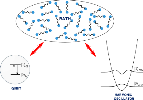
In this paper we focus on a bipartite system consisting of a two level system (qubit) and a harmonic oscillator interacting with the same bath of harmonic oscillators. The qubit is interacting with the bath via Jaynes-Cummings interaction type, whereas the position of the oscillator is coupled to the position of the bath via dipole interaction. The schematic diagram for the considered model is shown in Figure 1. A microscopic derivation is given for the master equation describing the open dynamics of the system considered in this model, which turns out to be in the form of the Gorini-Kossakowski-Sudarshan-Lindblad (GKSL) equation gorini1976completely ; lindblad1976generators . We follow hu2011necessary ; benatti2008environment ; benatti2003environment to show that this bath mediated interaction can lead to the generation of non-classical correlations including entanglement. We then find out the class of initial states which get entangled due to this bath mediated interaction. The dependence of entanglement generation on temperature of the bath in this scenario is shown. The entanglement measure, Negativity eisert2006entanglement ; vidal2002computable is used to study the entanglement dynamics of our system with respect to the relative coupling strength of qubit-bath coupling and oscillator-bath coupling. Weaker forms of quantum correlations are also studied using mutual information and quantum discord.

The outline of the paper is as follows. In Sect. 2 we express the Hamiltonian of the system of qubit and the harmonic oscillator and its interaction Hamiltonian. We then derive the master equation for the system. In Sect. 3 we discuss the possibility of generation of quantum correlations in the system and we find out the classes of initial which lead to entanglement. In Sect. 4 we study the dynamics of entanglement, mutual information and discord. We conclude in Sect. 5.

We work in units of $\hbar$ and $k_{B}$ set to 1. The total Hamiltonian $H_{T}$ for the composite system is,

$$H_{T}=H_{S}+H_{B}+H_{I},$$

(1)

where $H_{S}$, $H_{B}$ and $H_{I}$ are the Hamiltonian for the system, bath and interaction respectively. The system under consideration is a qubit and the harmonic oscillator interacting resonantly with the bath. The system Hamiltonian is therefore a sum of $H_{Q}$ and $H_{HO}$, that of the qubit and the harmonic oscillator, respectively.

$\displaystyle H_{S}$

$\displaystyle=H_{Q}+H_{HO}.$

(2)

Introducing ladder operators $a$ and $a^{\dagger}$ for the oscillator and excluding the zero-point energy, $H_{S}$ can be written as

$$H_{S}=\frac{\Omega}{2}\sigma_{z}+\Omega a^{\dagger}a.$$

(3)

The bath is modeled as a collection of independent harmonic oscillators and the Hamiltonian is

$$H_{B}=\sum_{k}\omega_{k}b_{k}^{\dagger}b_{k},$$

(4)

where $b_{k}^{\dagger}$ and $b_{k}$ are the bosonic creation and annihilation operators obeying the standard commutation relation $[b_{k},b_{k^{\prime}}^{\dagger}]=\delta_{k,k^{\prime}}$. The interaction between the system and the bath is assumed as follows. The qubit interacts with the bath via a Jaynes-Cummings interaction type, which indicates a radiative damping by its interaction with the many modes of the bath of harmonic oscillators. Also, the position of the oscillator is coupled to the position of the bath via dipole interaction. After the rotating-wave approximations are introduced, the total interaction Hamiltonian is expressed as

$$H_{I}=\sum_{k}g_{1}(\sigma_{+}b_{k}+\sigma_{-}{b}_{k}^{\dagger})+g_{2}(a^{\dagger}b_{k}+ab_{k}^{\dagger}),$$

(5)

where $\sigma_{+(-)}$ is the qubit raising (lowering) operator. $g_{1}$ and $g_{2}$ are the coupling constants corresponding to qubit-bath coupling and oscillator-bath coupling respectively. The interaction Hamiltonian in the interaction picture, $\tilde{H}_{I}$ is obtained as

	$\displaystyle\tilde{H}_{I}=\sum_{k}g_{1}(\sigma_{+}e^{\imath\Omega t}b_{k}e^{-\imath\omega_{k}t}+\sigma_{-}e^{-\imath\Omega t}{b}_{k}^{\dagger}e^{\imath\omega_{k}t})$
	$\displaystyle+g_{2}(a^{\dagger}e^{\imath\Omega t}b_{k}e^{-\imath\omega_{k}t}+ae^{-\imath\Omega t}b_{k}^{\dagger}e^{\imath\omega_{k}t}).$		(6)

Introducing the operators

	$\displaystyle S_{1}=\sigma_{+}e^{\imath\Omega t},\thinspace\thinspace\thinspace$		$\displaystyle B_{1}=\sum_{k}g_{1}b_{k}e^{-\imath\omega_{k}t},$
	$\displaystyle S_{2}=\sigma_{-}e^{-\imath\Omega t},\thinspace\thinspace\thinspace$		$\displaystyle B_{2}=\sum_{k}g_{1}b_{k}^{\dagger}e^{\imath\omega_{k}t},$
	$\displaystyle S_{3}=a^{\dagger}e^{\imath\Omega t},\thinspace\thinspace\thinspace$		$\displaystyle B_{3}=\sum_{k}g_{2}b_{k}e^{-\imath\omega_{k}t},$
	$\displaystyle S_{4}=ae^{-\imath\Omega t},\thinspace\thinspace\thinspace$		$\displaystyle B_{4}=\sum_{k}g_{2}b_{k}^{\dagger}e^{\imath\omega_{k}t}.$

The interaction Halmiltonian $\tilde{H}_{I}$ can be written as

$\displaystyle\tilde{H}_{I}=\sum_{i=1}^{4}S_{i}B_{i},$

(8)

where $S$ and $B$ refer to operators pertaining to the space of operators on the system and bath respectively. Assuming weak coupling with the bath, we use the Born-Markov approximation to obtain the master equation for the reduced density matrix of the system.

Defining the bath-correlation functions as $F_{ij}(t,s)=\langle B_{i}(t)B_{j}(s)\rangle=\mbox{Tr}_{B}(B_{i}(t)B_{j}(s)\rho_{B})$ and assuming that the bath is in an equilibrium state so that $F_{ij}(t,s)=F_{ij}(t-s)$ and using the form of Eq. (8), one obtains the master equation in the Schrödinger picture as follows.

	$\displaystyle\frac{\partial\rho_{S}(t)}{\partial t}=-\imath~{}[H_{S},\rho_{S}(t)]-\sum_{\begin{subarray}{c}i,j=1\\ \end{subarray}}^{4}\int_{0}^{\infty}d\tau~{}\Big{(}[S_{i},S_{j}(-\tau)\rho_{S}(t)]F_{ij}(\tau)$
	$\displaystyle+[\rho_{S}(t)S_{j}(-\tau),S_{i}]F_{ji}(-\tau)\Big{)}.$		(9)

Let’s define

	$\displaystyle\int_{0}^{\infty}d\tau e^{\imath\Omega\tau}F_{12}(\tau)$	$\displaystyle=\Gamma_{1}=\gamma_{1}+\imath\delta_{1},$			(10)
	$\displaystyle\int_{0}^{\infty}d\tau e^{\imath\Omega\tau}F_{21}(-\tau)$	$\displaystyle=\Gamma_{2}=\gamma_{2}+\imath\delta_{2}.$			(11)

where $\{\gamma_{1},\gamma_{2},\delta_{1},\delta_{2}\}\in\mathbbm{R}$. The real parts $\gamma_{1}$ and $\gamma_{2}$ are given by $\zeta\frac{\exp(1/T)}{\exp(1/T)-1}$ and $\zeta\frac{1}{\exp(1/T)-1}$ respectively, where $\zeta$ is the spontaneous emission constant and temperature of the bath $T$ is given in the units of $\Omega$. Now one can see that

	$\displaystyle\int_{0}^{\infty}d\tau e^{\imath\Omega\tau}F_{41}(-\tau)=\int_{0}^{\infty}d\tau e^{\imath\Omega\tau}F_{23}(-\tau)=\frac{g_{2}}{g_{1}}\Gamma_{2},$		(12)
	$\displaystyle\int_{0}^{\infty}d\tau e^{\imath\Omega\tau}F_{14}(\tau)=\int_{0}^{\infty}d\tau e^{\imath\Omega\tau}F_{32}(\tau)=\frac{g_{2}}{g_{1}}\Gamma_{1},$		(13)
	$\displaystyle\int_{0}^{\infty}d\tau e^{\imath\Omega\tau}F_{34}(\tau)=\frac{g_{2}^{2}}{g_{1}^{2}}\Gamma_{1},$		(14)
	$\displaystyle\int_{0}^{\infty}d\tau e^{\imath\Omega\tau}F_{43}(-\tau)=\frac{g_{2}^{2}}{g_{1}^{2}}\Gamma_{2}.$		(15)

The remaining terms which are of the form $\mbox{Tr}_{B}(b_{k}e^{-\imath\Omega_{k}t}b_{k}e^{-\imath\Omega_{k}s}\rho_{B})$ or
$\mbox{Tr}_{B}(b_{k}^{\dagger}e^{-\imath\Omega_{k}t}b_{k}^{\dagger}e^{-\imath\Omega_{k}s}\rho_{B})$ are equal to zero since we assumed the bath is in an equilibrium state. After substituting Eq. (II) and Eq. (12-15) into Eq. (II) and neglecting the contributions from $\delta_{1}$ and $\delta_{2}$, one obtains the master equation,

	$\displaystyle\frac{\partial}{\partial t}\rho_{S}(t)=-\imath~{}[\frac{\Omega}{2}\sigma_{z},\rho_{S}(t)]+\gamma_{1}\Big{(}2\sigma_{-}\rho_{S}(t)\sigma_{+}-\{\sigma_{+}\sigma_{-},\rho_{S}(t)\}\Big{)}$
	$\displaystyle+\gamma_{2}\Big{(}2\sigma_{+}\rho_{S}(t)\sigma_{-}-\{\sigma_{-}\sigma_{+},\rho_{S}(t)\}\Big{)}-\imath~{}[\Omega a^{\dagger}a,\rho_{S}(t)]$
	$\displaystyle+\gamma_{1}\eta^{2}\Big{(}2a\rho_{S}(t)a^{\dagger}-\{a^{\dagger}a,\rho_{S}(t)\}\Big{)}+\gamma_{2}\eta^{2}\Big{(}2a^{\dagger}\rho_{S}(t)a-\{aa^{\dagger},\rho_{S}(t)\}\Big{)}$
	$\displaystyle\left.\begin{array}[]{r}+\gamma_{1}\eta\Big{(}2\sigma_{-}\rho_{S}(t)a^{\dagger}+2a\rho_{S}(t)\sigma_{+}-\{\sigma_{+}a,\rho_{S}(t)\}-\{a^{\dagger}\sigma_{-},\rho_{S}(t)\}\Big{)}\\ +\gamma_{2}\eta\Big{(}2\sigma_{+}\rho_{S}(t)a+2a^{\dagger}\rho_{S}(t)\sigma_{-}-\{a\sigma_{+},\rho_{S}(t)\}-\{\sigma_{-}a^{\dagger},\rho_{S}(t)\}\Big{)}\end{array}\right.$		(18)

where $\eta=g_{2}/g_{1}$ is the ratio of coupling strengths between qubit-bath coupling and oscillator-bath coupling.

We consider the single excitation sector for the Harmonic Oscillator so as to make use of Positive Partial Transpose criterion (P.P.T) peres1996separability ; horodecki2001separability in showing that the dynamics described by Eq. (II) is entangling. One could consider the second excitation sector of the oscillator which would map the problem to the case of a qubit-qutrit interaction. However, we do not address it in the present study. We denote the eigenstate of lowest energy level by $\ket{0}_{HO}$ and the eigenstate of highest energy level by $\ket{1}_{HO}$ as shown in Figure 1. We replace $a$ and $a^{\dagger}$ with $\sigma_{-}^{\scaleto{HO}{3pt}}$ and $\sigma_{+}^{\scaleto{HO}{3pt}}$ respectively as they are acting on a qubit. For clarity, we replace $\sigma_{+}$ and $\sigma_{-}$ with $\sigma_{+}^{\scaleto{Q}{4pt}}$ and $\sigma_{-}^{\scaleto{Q}{4pt}}$ respectively. One then obtains the master equation (II),

	$\displaystyle\frac{\partial}{\partial t}\rho_{S}(t)=$	$\displaystyle-\imath~{}[\frac{\Omega}{2}\sigma_{z},\rho_{S}(t)]+L_{Q}[\rho(t)]-\imath~{}[\Omega\sigma_{+}^{\scaleto{HO}{3pt}}\sigma_{-}^{\scaleto{HO}{3pt}},\rho_{S}(t)]+L_{HO}[\rho(t)]$			(19)
		$\displaystyle+L_{QHO}[\rho(t)],$

where

	$\displaystyle L_{Q}[\rho(t)]=\gamma_{1}\Big{(}2\sigma_{-}^{\scaleto{Q}{4pt}}\rho_{S}(t)\sigma_{+}^{\scaleto{Q}{4pt}}-\{\sigma_{+}^{\scaleto{Q}{4pt}}\sigma_{-}^{\scaleto{Q}{4pt}},\rho_{S}(t)\}\Big{)}$
	$\displaystyle+\gamma_{2}\Big{(}2\sigma_{+}^{\scaleto{Q}{4pt}}\rho_{S}(t)\sigma_{-}^{\scaleto{Q}{4pt}}-\{\sigma_{-}^{\scaleto{Q}{4pt}}\sigma_{+}^{\scaleto{Q}{4pt}},\rho_{S}(t)\}\Big{)},$		(20)

	$\displaystyle L_{HO}[\rho(t)]=\gamma_{1}\eta^{2}\Big{(}2\sigma_{-}^{\scaleto{HO}{3pt}}\rho_{S}(t)\sigma_{+}^{\scaleto{HO}{3pt}}-\{\sigma_{+}^{\scaleto{HO}{3pt}}\sigma_{-}^{\scaleto{HO}{3pt}},\rho_{S}(t)\}\Big{)}$
	$\displaystyle+\gamma_{2}\eta^{2}\Big{(}2\sigma_{+}^{\scaleto{HO}{3pt}}\rho_{S}(t)\sigma_{-}^{\scaleto{HO}{3pt}}-\{\sigma_{-}^{\scaleto{HO}{3pt}}\sigma_{+}^{\scaleto{HO}{3pt}}\rho_{S}(t)\}\Big{)},$		(21)

and

	$\displaystyle L_{QHO}[\rho(t)]=\gamma_{1}\eta\Big{(}2\sigma_{-}^{\scaleto{Q}{4pt}}\rho_{S}(t)\sigma_{+}^{\scaleto{HO}{3pt}}-\{\sigma_{+}^{\scaleto{HO}{3pt}}\sigma_{-}^{\scaleto{Q}{4pt}},\rho_{S}(t)\}\Big{)}$
	$\displaystyle+\gamma_{1}\eta\Big{(}2\sigma_{-}^{\scaleto{HO}{3pt}}\rho_{S}(t)\sigma_{+}^{\scaleto{Q}{4pt}}-\{\sigma_{+}^{\scaleto{Q}{4pt}}\sigma_{-}^{\scaleto{HO}{3pt}},\rho_{S}(t)\}\Big{)}$
	$\displaystyle+\gamma_{2}\eta\Big{(}2\sigma_{+}^{\scaleto{Q}{4pt}}\rho_{S}(t)\sigma_{-}^{\scaleto{HO}{3pt}}+2\sigma_{+}^{\scaleto{HO}{3pt}}\rho_{S}(t)\sigma_{-}^{\scaleto{Q}{4pt}}-\{\sigma_{-}^{\scaleto{HO}{3pt}}\sigma_{+}^{\scaleto{Q}{4pt}},\rho_{S}(t)\}-\{\sigma_{-}^{\scaleto{Q}{4pt}}\sigma_{+}^{\scaleto{HO}{3pt}},\rho_{S}(t)\}\Big{)}.$

The terms $L_{Q}[\rho(t)]$ and $L_{HO}[\rho(t)]$ of the master equation (19) describe the dissipation of the qubits $Q$ and $HO$ respectively. The term $L_{QHO}[\rho(t)]$ includes the coupling between the qubits $Q$ and $HO$ induced by the bath.

The master equation (19) can be decomposed into 16 differential equations, one for each entry of the density matrix. Using this one can derive a dynamical equation of evolution for the density matrix. We use this to look at the dynamics of quantum correlations in the system in Sect. 3 and Sect. 4.

Bennati et al. benatti2008environment ; benatti2003environment give the conditions for a semigroup to entangling. We make use of the result to show that the dynamics described by Eq. (19), which is stemming from a combination of Jaynes-Cummings interaction and dipole interaction as described in Sect. 1, is entangling. We further analytically find out the class of initial states of the system which lead to entanglement as $t\rightarrow 0^{+}$.

The master equation of the system, which is effectively a pair of two-level systems ($Q$ and $HO$), is in a GKSL gorini1976completely form:

$\displaystyle\partial_{t}\rho(t)=-\imath[H,\rho(t)]+L[\rho(t)],$

(23)

where $H$, which is equal to $H_{S}$ in our case, is the effective system Hamiltonian, while

$\displaystyle L[\rho(t)]=\sum_{i,j}\mathcal{K}_{ij}\left[\mathcal{G}_{i}\rho(t)\mathcal{G}_{j}^{\dagger}-\frac{1}{2}\{\mathcal{G}_{j}^{\dagger}\mathcal{G}_{i},\rho(t)\}\right],$

(24)

is the dissipative term and $\{\mathcal{G}_{i}\}_{\{i=1\dots d^{2}-1\}}$ can be any trace orthonormal basis. By comparing with Eq. (19), one can see that

	$\displaystyle\mathcal{G}_{1}=\sigma_{+}^{\scaleto{Q}{4pt}}\otimes\mathbbm{1}^{\scaleto{HO}{3pt}},$
	$\displaystyle\mathcal{G}_{2}=\sigma_{-}^{\scaleto{Q}{4pt}}\otimes\mathbbm{1}^{\scaleto{HO}{3pt}},$
	$\displaystyle\mathcal{G}_{3}=\mathbbm{1}^{\scaleto{Q}{4pt}}\otimes\sigma_{-}^{\scaleto{HO}{3pt}},$
	$\displaystyle\mathcal{G}_{4}=\mathbbm{1}^{\scaleto{Q}{4pt}}\otimes\sigma_{+}^{\scaleto{HO}{3pt}}.$		(25)

The co-efficients $\mathcal{K}_{ij}$ form Kossakowski Matrix ($\mathcal{K}$) kossakowski72

$$\mathcal{K}=\matrixquantity(2\gamma_{2}&0&0&2\eta\gamma_{2}\\ 0&2\gamma_{1}&2\eta\gamma_{1}&0\\ 0&2\eta\gamma_{1}&2\eta^{2}\gamma_{1}&0\\ 2\eta\gamma_{2}&0&0&2\eta^{2}\gamma_{2}),$$

(26)

which is Hermitian i.e. $\mathcal{K}=\mathcal{K}^{\dagger}$.

The dissipative contribution of $L[\rho(t)]$ is written as

$$L[\rho(t)]=L_{Q}[\rho(t)]+L_{HO}[\rho(t)]+L_{QHO}[\rho(t)].$$

(27)

According hu2011necessary , the dynamics generate non-classical correlations between the qubits $Q$ and $HO$ since $L_{QHO}[\rho(t)]\neq 0$. This is very intuitive because $L_{QHO}[\rho(t)]$ includes the induced coupling between the qubits $Q$ and $HO$.

Since non-classical correlations do not imply entanglement, we now specifically check if the dynamics described by Eq. (19) is entangling. According to the Positive Partial Transpose criterion peres1996separability ; horodecki2001separability , the system $\rho$ is separable if and only if $\rho^{T_{HO}}$ is positive semi definite, where $\rho^{T_{HO}}$ denotes the partial transposition on $\rho$ with respect to the subsystem $HO$. One can then define the following quantity

$\displaystyle\Xi(t)=\bra{\psi}\rho^{T_{HO}}(t)\ket{\psi},$

(28)

to look for negative eigenvalues in $\rho^{T_{HO}}(t)$. So $\Xi(t)<0$ implies $\rho(t)$ is entangled.

From benatti2008environment ; benatti2003environment , we know that the evolution described by Eq. (19) generates entanglement if and only if there exist a separable initial state $\rho(0)$ and a vector $\ket{\psi}\in\mathbbm{C}^{4}$ such that the conditions

	$\displaystyle\Xi(0)=0$		(29)
	$\displaystyle\partial_{t}\Xi(0)<0$		(30)

are satisfied. This also implies that the system starting in the separable state $\rho(0)$ gets entangled as $t\rightarrow 0^{+}$ because the condition $\partial_{t}\Xi(0)<0$ along with $\Xi(0)=0$ implies that $\lim\limits_{t\rightarrow 0^{+}}\Xi(t)<0$. We consider the case where the system starts in $\ket{0}_{Q}\ket{1}_{HO}$ to show that the conditions (29) and (30) can be satisfied. We choose $\ket{\psi}=\kappa_{1}\ket{0}_{Q}\ket{0}_{HO}+\kappa_{2}\ket{1}_{Q}\ket{0}_{HO}+\kappa_{3}\ket{1}_{Q}\ket{1}_{HO}$ according to condition Eq. (29). For this $\ket{\psi}$,

$$\partial_{t}\Xi(0)=2\gamma_{1}\kappa_{1}^{2}\eta^{2}-2(\gamma_{1}+\gamma_{2})\kappa_{1}\kappa_{3}\eta+2\gamma_{2}\kappa_{3}^{2}.$$

(31)

The above equation, which is quadratic in $\kappa_{1}$(or $\kappa_{3}$) has two roots unless $\gamma_{1}=\gamma_{2}$. Since one can find $\kappa_{1}$ and $\kappa_{3}$ for a given $\gamma_{1},\gamma_{2}$ and $\eta$ such that condition (30) is satisfied, the system gets entangled and the considered dynamics in Eq. (19) are entangling. For example, when $\gamma_{1}=1.01,\gamma_{2}=0.01$ and $\Omega=0.001$, one can see that $\kappa_{1}=1$ and $\kappa_{3}=-1/2$ satisfy condition (30).

We consider the following general form for the initial pure and separable state of the system

$\displaystyle\ket{\phi}=(p\ket{0}+\sqrt{1-p^{2}}\ket{1})_{Q}\otimes(q\ket{0}+\sqrt{1-q^{2}}\ket{1})_{HO},$

(32)

where $p,q\in[-1,1]$, to find the subset of states which generate entanglement as $t\rightarrow 0^{+}$ when evolved according to Eq. (II). We first choose a general $\ket{\psi}$ which satisfies condition (29)

	$\displaystyle\ket{\psi}=\alpha\left((\sqrt{1-p^{2}}\ket{0}-p\ket{1})\otimes(q\ket{0}+\sqrt{1-q^{2}}\ket{1})\right)$
	$\displaystyle+\beta\left((p\ket{0}+\sqrt{1-p^{2}}\ket{1})\otimes(\sqrt{1-q^{2}}\ket{0}-q\ket{1})\right)$
	$\displaystyle+\vartheta\left((\sqrt{1-p^{2}}\ket{0}-p\ket{1})\otimes(\sqrt{1-q^{2}}\ket{0}-q\ket{1})\right).$		(33)

For this $\ket{\psi}$ and $\rho(0)=\outerproduct{\phi}{\phi}$, we find

$\displaystyle\begin{array}[]{c}\partial_{t}\Xi(0)=2\left(\gamma_{2}p^{4}+\left(p^{2}-1\right)^{2}\gamma_{1}\right)\alpha^{2}+2\beta^{2}\eta^{2}\left(\gamma_{2}q^{4}+\left(q^{2}-1\right)^{2}\gamma_{1}\right)\\ -2\left(\left(p^{2}\left(2q^{2}-1\right)-q^{2}\right)\beta\eta\left(\gamma_{1}+\gamma_{2}\right)\alpha\right).\\ \end{array}$

(36)

For the initial settings $\gamma_{1}=1.01,\gamma_{2}=0.01$ and $\Omega=0.001$, the Eq. (36) is reduced to

$\displaystyle\begin{array}[]{c}\partial_{t}\Xi(0)=\frac{1}{50}\left(\alpha^{2}\left(102p^{4}-202p^{2}+101\right)+102\alpha\beta\eta\left(p^{2}\left(1-2q^{2}\right)+q^{2}\right)\right)\\ +\frac{1}{50}\left(\beta^{2}\eta^{2}\left(102q^{4}-202q^{2}+101\right)\right).\\ \end{array}$

(39)

One can find the set of all $(p,q)$, where $p,q\in[-1,1]$, for which there exists at least one 3-tuple $(\alpha,\beta,\vartheta)$ such that the condition (30) is satisfied. These set of points $(p,q)$ are plotted in Figure 2.

Note that even if one includes the contributions of $\delta_{1}$ and $\delta_{2}$, which are the bath-induced Lamb shifts, the above result is not affected due the fact that the quantity $\partial_{t}\Xi(0)$ (Eq. (36)) remains the same.

In this section, the dynamics of quantum correlations in the two effective qubit system interacting with the bath are studied with respect to $\zeta t$ which we denote by $t$ for brevity.

We study the quantum correlations between a qubit and a harmonic oscillator, not interacting directly, but coupled to a common bath. To this end, we first obtain the microscopic derivation of the master equation for the open dynamics of the system, modelled as a qubit and a harmonic oscillator, with a single excitation sector, interacting with the bath via Jaynes-Cummings interaction type. We make use of the necessary and sufficient conditions given in hu2011necessary ; benatti2008environment ; benatti2003environment to show these dynamics generate non-classical correlations including entanglement. We further analytically find out the class of initial states which generate entanglement. One can do a similar study by considering the second excitation sector for the harmonic oscillator which effectively makes the system a composition of a qubit and qutrit. Entanglement is quantified using negativity eisert2006entanglement ; vidal2002computable and its dependence on the temperature of the bath is shown. Other measures of quantum correlations studied include mutual information and quantum discord. We note that the entanglement generated persists for long time, making the system potentially useful for practical applications.

The authors would like to thank Dr. Camille Lombard Latune for insightful comments and suggestions. The work of V. J. and F. P. is based upon research supported by the South African Research Chair Initiative of the Department of Science and Technology and National Research Foundation. R. S. thanks DST-SERB, Govt. of India, for financial support provided through the project EMR/2016/004019.

References

- (1) Breuer, H.-P. and Petruccione, F. The Theory of Open Quantum Systems. Oxford University Press, (2002).
- (2) Rivas, A. and Huelga, S. F. Open Quantum Systems. Springer, (2012).
- (3) Haroche, S. and Raimond, J.-M Exploring the Quantum: Atoms, Cavities, and Photons. Oxford University Press, (2006).
- (4) Jagadish, V. and Petruccione, F. Quanta, 7(1):54–67, 2018.
- (5) Ma, J., Sun, Z., Wang, X., and Nori, F. Phys. Rev. A 85(6), 062323 (2012).
- (6) Braun, D. Phys. Rev. Lett. 89(27), 277901 (2002).
- (7) Contreras-Pulido, L. and Aguado, R. Phys. Rev. B 77(15), 155420 (2008).
- (8) Banerjee, S., Ravishankar, V., and Srikanth, R. Ann. Phys. 325(4), 816–834 (2010).
- (9) Banerjee, S., Ravishankar, V., and Srikanth, R. Eur. Phys. J. D 56(2), 277–290 (2010).
- (10) Paz, J. P. and Roncaglia, A. J. Phys. Rev. Lett. 100(22), 220401 (2008).
- (11) Su, S.-L., Shao, X.-Q., Wang, H.-F., and Zhang, S. Phys. Rev. A 90(5), 054302 (2014).
- (12) Utami, D. W. and Clerk, A. Phys. Rev. A 78(4), 042323 (2008).
- (13) Leibfried, D., Blatt, R., Monroe, C., and Wineland, D. Rev. Mod. Phys. 75(1), 281 (2003).
- (14) Cirac, J. I. and Zoller, P. Phys. Rev. Lett. 74(20), 4091 (1995).
- (15) Wineland, D. J., Barrett, M., Britton, J., Chiaverini, J., DeMarco, B., Itano, W. M., Jelenković, B., Langer, C., Leibfried, D., Meyer, V., et al. Philos. Trans. Royal Soc. A. Math. Phys. Eng. Sci. 361(1808), 1349–1361 (2003).
- (16) Sørensen, A. and Mølmer, K. Phys. Rev. Lett. 82(9), 1971 (1999).
- (17) Raimond, J.-M., Brune, M., and Haroche, S. Rev. Mod. Phys. 73(3), 565 (2001).
- (18) Osnaghi, S., Bertet, P., Auffeves, A., Maioli, P., Brune, M., Raimond, J.-M., and Haroche, S. Phys. Rev. Lett. 87(3), 037902 (2001).
- (19) Cubitt, T. S., Verstraete, F., Dür, W., and Cirac, J. I. Phys. Rev. Lett. 91(3), 037902 (2003).
- (20) Gorini, V., Kossakowski, A., and Sudarshan, E. C. G. J. Math. Phys. 17(5), 821–825 (1976).
- (21) Lindblad, G. Commun. Math. Phys. 48(2), 119–130 (1976).
- (22) Hu, X., Gu, Y., Gong, Q., and Guo, G. Phys. Rev. A 84(2), 022113 (2011).
- (23) Benatti, F., Liguori, A. M., and Nagy, A. J. Math. Phys. 49(4), 042103 (2008).
- (24) Benatti, F., Floreanini, R., and Piani, M. Phys. Rev. Lett. 91(7), 070402 (2003).
- (25) Kossakowski, A. Rep. Math. Phys. 3, 247–274 (1972).
- (26) Eisert, J. arXiv preprint quant-ph/0610253 (2006).
- (27) Vidal, G. and Werner, R. F. Phys. Rev. A 65(3), 032314 (2002).
- (28) Peres, A. Phys. Rev. Lett. 77(8), 1413 (1996).
- (29) Horodecki, M., Horodecki, P., and Horodecki, R. Phys. Lett. A 283(1-2), 1–7 (2001).
- (30) Henderson, L. and Vedral, V. J. Phys. A: Math. Gen. 34(35), 6899 (2001).
- (31) Ollivier, H. and Zurek, W. H. Phys. Rev. Lett. 88(1), 017901 (2001).