^†^†thanks: [email protected]

Dynamics of k-essence in loop quantum cosmology

Jiali Shi¹ Jian-Pin Wu² ¹ College of Physical Science and Technology, Bohai University, Jinzhou 121013, China
² Center for Gravitation and Cosmology, College of Physical Science and Technology, Yangzhou University, Yangzhou 225009, China

Abstract

In this paper, we study the dynamics of k-essence in loop quantum cosmology (LQC). The study indicates that the loop quantum gravity (LQG) effect plays a key role only in the early epoch of the universe and is diluted at the later stage. The fixed points in LQC are basically consistent with that in standard Friedmann-Robertson-Walker (FRW) cosmology. For most of the attractor solutions, the stability conditions in LQC are in agreement with that for the standard FRW universe. But for some special fixed point, more tighter constraints are imposed thanks to the LQG effect.

I Introduction

Numerous cosmological observations strongly suggest that the universe is undergoing accelerated expansion at present epoch Riess:1998cb ; Perlmutter:1998np ; Bennett:2003bz ; Spergel:2003cb ; Tegmark:2003ud ; Tegmark:2003uf . It is the most widely accepted idea that a mysterious dominant component, dark energy with negative pressure, drives this cosmic acceleration. The most popular dark energy model is quintessence. It is described by a canonical scalar field accompanying with a particular potential that results in the late time acceleration of the universe. However, there has been a growing interest in the study of alternative models characterized by a non-canonical kinetic term, and has made a great progress. This scenario was originally proposed to drive the inflation in the early universe ArmendarizPicon:1999rj ; Garriga:1999vw . And then, it was first applied to describe late time cosmic acceleration in Chiba:1999ka . More general formalism of scalar field dark energy model was proposed in ArmendarizPicon:2000dh ; ArmendarizPicon:2000ah and we call it as k-essence.

As we all known, the scalar field dynamical dark energy models suffer from the so-called fine-tuning problem and coincidence problem. To attack these problems, we can resort to the scalar field models exhibiting scaling solutions, see Tsujikawa:2006mw ; Gong:2006sp ; Ferreira:1997hj ; Copeland:1997et ; Guo:2003rs ; Guo:2003eu ; Lin:2020fue and therein (also see Copeland:2006wr for a review). As a dynamical attractor, the scaling solution can partly alleviate these two problems. In addition, we can also study the stability conditions of the scalar field dynamical dark energy models, see for example UrenaLopez:2005zd ; Carot:2002ww ; Ito:2012 .

Lots of dynamical dark energy models, including k-essence, have been deeply studied in the framework of the standard cosmology. However, it is expected that in the regime of very high curvature, the general relativity (GR) breaks down and the big bang singularity emerges. A theory of quantum gravity shall provide us a natural scenario to attach this problem. One of the candidate theories of quantum gravity is loop quantum gravity (LQG), a non-perturbative and background-independent quantum gravity theory LQGRovelli ; LQGThiemann ; Ashtekar:2004eh ; Han:2005km . Based on the LQG, we can construct a symmetry-reduced cosmological model with homogeneous and isotropic spacetimes, known as loop quantum cosmology (LQC) Bojowald:2001xe ; Ashtekar:2006rx ; Ashtekar:2006wn ; Bojowald:2006da ; Ashtekar:2003hd ; Ashtekar:2011ni . The non-perturbative quantum gravity effects result in a $-\rho^{2}$ modification to the standard Friedmann dynamics. The big bang singularity in the early universe can be resolved in this scenario Bojowald:2001xe ; Ashtekar:2003hd ; Ashtekar:2006rx ; Ashtekar:2006uz ; Bojowald:2003xf ; Singh:2003au ; Vereshchagin:2004uc ; Date:2005nn ; Date:2004fj ; Goswami:2005fu . It is very interesting to notice that even at the semi-classical level, instead of the big bang singularity, a big bounce emerges Bojowald:2005zk ; Stachowiak:2006uh . The LQG effect also results in the emergences of the super-inflationary phase Bojowald:2002nz . The horizon problem with only a few number of e-foldings can be resolved in this landscape Copeland:2007qt . Further, to search for the potential observable prints, the cosmological perturbative theory in LQC is also deeply explored in Bojowald:2006tm ; Bojowald:2006zb ; Bojowald:2008gz ; Bojowald:2007hv ; Bojowald:2007cd ; Wu:2010wj ; Wu:2012mh ; Wu:2018mhg and the primordial power spectrum is studied in Copeland:2007qt ; Hossain:2004wm ; Calcagni:2006pr ; Mulryne:2006cz ; Zhang:2007bi ; Artymowski:2008sc ; Tsujikawa:2003vr ; Shimano:2009tn . In addition, the large scale effect of LQG is also found in Ding:2008tq , which provides us the possibility to study the LQG effect on the dark energy evolution. Many scalar field dark energy models and their dynamics have been widely studied in the framework of LQC, see Wei:2007rp ; Wu:2008db ; Fu:2008gh ; Chen:2008ca ; Zonunmawia:2017ofc ; Li:2010ju and therein.

In this paper, we study the dynamics of k-essence and its attractor solutions in LQC. Our paper is organized as what follows. In Section II, we introduce the k-essence in the LQC framework and derive the equations of motion of the dynamical system. And then, we study the dynamics of k-essence for the constant coupling parameters and dynamical changing coupling parameters in Section III and Section IV, respectively. The conclusions and discussions are briefly presented in Section V.

II K-essence in LQC

In quintessence scalar field dark energy model, the potential energy of the scalar field plays a key role in driving the cosmic late-time acceleration. If we introduce a non-canonical kinetic energy term in the Lagrangian, we find that even when the potential vanishes, the cosmic acceleration can also achieved. This model characterized by a non-canonical kinetic energy term is called as k-essence. The most general Lagrangian of k-essence is a function of the scalar field $\phi$ and its kinetic energy term $X\equiv\frac{1}{2}\partial_{\mu}\phi\partial^{\mu}\phi$ , i.e., $\mathcal{L}=f(\phi,X)$ . In this paper, we consider a specific form of k-essence as ArmendarizPicon:2000dh ; ArmendarizPicon:2000ah ; Chakraborty:2019swx

\displaystyle\mathcal{L}=\alpha(\phi)X+\beta(\phi)X^{2}-V(\phi)\,,

(1)

where $V(\phi)$ is the potential, and the coefficients $\alpha$ and $\beta$ are the functions of scalar field. The above Lagrangian is a polynomial of degree $2$ in the kinetic energy $X$ . This type of Lagrangian can emerge from the low-energy effective string theory ArmendarizPicon:1999rj ; Garriga:1999vw .

Incorporating the LQG effect, instead of the standard Friedmann equation, we have an effective one Bojowald:2001xe ; Ashtekar:2006rx ; Ashtekar:2006wn ; Bojowald:2006da ; Ashtekar:2003hd ; Ashtekar:2011ni ¹¹1We would like to point out that there is an alternative version of modified Friedmann equation proposed in Ding:2008tq ; Yang:2009fp , which could be derived from full LQG as recently shown by Assanioussi:2018hee .

\displaystyle H^{2}={\frac{\rho_{t}}{3M_{p}^{2}}}\Big{(}1-{\frac{\rho_{t}}{\rho_{c}}}\Big{)}\,,

(2)

where $H\equiv\dot{a}/a$ is the Hubble parameter and $\rho_{t}$ is the total energy density of the cosmological contents. $M_{p}^{2}=\frac{1}{8\pi G}$ is the square of Plank mass. In what follows, we set $M_{p}^{2}=1$ for convenience. $\rho_{c}={\sqrt{3}}/(16{\pi}{\gamma}^{3}G^{2}{\hbar})$ is the critical density where $\gamma$ is the dimensionless Barbero-Immirzi parameter and $\hbar$ is Plank constant. Along with the conservation law

\displaystyle\dot{\rho_{t}}+3H({\rho_{t}}+p_{t})=0\,,

(3)

the effective Friedmann equation provides a description of the universe incorporating the LQG effect. $p_{t}$ in the above equation is the total pressure. Differentiating the Friedmann equation (2) and using the conservation law (3), one achieves the following effective Raychaudhuri equation

\displaystyle\dot{H}=-{\frac{(\rho_{t}+p_{t})}{2}}\Big{(}1-{\frac{2\rho_{t}}{\rho_{c}}}\Big{)}\,.

(4)

We assume that the contents of the universe include the k-essence scalar field and the dark matter. So the total energy density and pressure of the contents of the universe are

\displaystyle\rho_{t}=\rho_{\phi}+\rho_{m}\,,~{}~{}~{}~{}~{}~{}p_{t}=p_{\phi}+p_{m}\,,

(5)

where $\rho_{\phi}$ ( $\rho_{m}$ ) and $p_{\phi}$ ( $p_{m}$ ) are the energy density and pressure of the dark energy (dark matter), respectively. From the Lagrangian of k-essence (1), we can easily derive $\rho_{\phi}$ and $p_{\phi}$ in flat Friedmann-Robertson-Walker (FRW) background as ArmendarizPicon:2000dh ; ArmendarizPicon:2000ah ; Chakraborty:2019swx

	$\displaystyle\rho_{\phi}={\alpha(\phi)}X+3{\beta(\phi)}X^{2}+V{(\phi)}\,,\$		(6)
	$\displaystyle p_{\phi}={\alpha(\phi)}X+{\beta(\phi)}X^{2}-V{(\phi)}\,.$		(7)

Since we have assumed that the universe is homogeneity and isotropy, one has $X={\frac{1}{2}}{\dot{\phi}^{2}}$ where the dot denotes the derivative with respect to the time. Further, taking the variation of the Lagrangian (1) with respect to the scalar field $\phi$ , one obtains the Klein-Gordon (KG) equation as

\displaystyle\ddot{\phi}[{\alpha(\phi)}+3{\beta(\phi)}\dot{\phi}^{2}]+\alpha{{}^{\prime}}{(\phi)}{\frac{\dot{\phi}^{2}}{2}}+3{\beta{{}^{\prime}}(\phi)}{\frac{\dot{\phi}^{4}}{4}}+3H\dot{\phi}[{\alpha(\phi)}+{\beta(\phi)}\dot{\phi}^{2}]+V{{}^{\prime}}{(\phi)}=0\,.

(8)

To study the dynamics of the above system, we define the following set of dimensionless variables:

	$\displaystyle x={\frac{\alpha(\phi)\dot{\phi}^{2}}{6H^{2}}},~{}~{}~{}~{}y={\frac{\beta(\phi)\dot{\phi}^{4}}{12H^{2}}}\,,$
	$\displaystyle b={\frac{V(\phi)}{3H^{2}}},~{}~{}~{}~{}\lambda={\frac{1}{\alpha}}{\frac{d\alpha}{d\phi}}{\frac{\dot{\phi}}{H}}\,,$
	$\displaystyle\delta={\frac{1}{\beta}}{\frac{d\beta}{d\phi}}{\frac{\dot{\phi}}{H}},~{}~{}~{}~{}z={\frac{\rho_{t}}{\rho_{c}}}\,.$		(9)

In term of the above dimensionless variables, the effective Friedman equation (2) and Raychaudhuri equation (4) can be rewritten as

	$\displaystyle\frac{\rho_{m}}{3H^{2}}=\frac{1}{1-z}-(x+3y+b)\,,\$		(10)
	$\displaystyle\frac{\dot{H}}{H^{2}}=-\frac{3}{2}\Big{[}2x+4y+\frac{1-(x+3y+b)(1-z)}{1-z}\Big{]}(1-2z)\,.$		(11)

And then, we recast the above system into the following autonomous form

	$\displaystyle x{{}^{\prime}}=x{\lambda}+3x{\mathcal{G}}-2x{\mathcal{F}}\,,\$		(12)
	$\displaystyle y{{}^{\prime}}=y{\delta}+3y{\mathcal{G}}-4y{\mathcal{F}}\,,\$		(13)
	$\displaystyle b{{}^{\prime}}={\sigma}b+3b{\mathcal{G}}\,,\$		(14)
	$\displaystyle\lambda{{}^{\prime}}={\frac{3}{2}}{\lambda}{\mathcal{G}}-{\lambda}{\mathcal{F}}-{\lambda}^{2}(1-{\Gamma})\,,\$		(15)
	$\displaystyle\delta{{}^{\prime}}={\frac{3}{2}}{\delta}{\mathcal{G}}-{\delta}^{2}(1-{\tau})-{\delta}{\mathcal{F}}\,,\$		(16)
	$\displaystyle z{{}^{\prime}}=-3z(1+x+y+b(-1+z)-xz-yz)\,,$		(17)

where

	$\displaystyle\mathcal{F}={\frac{3(x+2y)}{x+6y}}+{\frac{x{\lambda}+3{\delta}y+{\sigma}b}{2(x+6y)}}\,,\$		(18)
	$\displaystyle\mathcal{G}={\frac{(-1+2z)(1+x+y+b(-1+z)-xz-yz)}{-1+z}}\,,$		(19)

and

\displaystyle\Gamma={\frac{\alpha({\frac{d^{2}{\alpha}}{d{\phi}^{2}}})}{({\frac{d{\alpha}}{d{\phi}}})^{2}}}\,,~{}~{}~{}~{}~{}\tau={\frac{\beta({\frac{d^{2}{\beta}}{d{\phi}^{2}}})}{({\frac{d{\beta}}{d{\phi}}})^{2}}}\,,~{}~{}~{}~{}~{}\sigma={\frac{d(ln~{}V)}{dN}}\,.

(20)

Notice that here we have introduced the number of e-folding $N\equiv\ln(a/a_{0})$ with $a_{0}$ being the current value of the scale factor and the prime represents the derivative with respect to $N$ in the above equations.

Comparing with the standard FRW cosmology, an additional dimensionless variable $z\equiv\rho_{t}/\rho_{c}$ is introduced to describe the system in LQC. The nonzero $z$ represents the LQG effect. Next, we shall treat $\lambda$ and $\delta$ as constant coupling parameters and dynamically changing variables respectively to study the dynamics of the system.

III Dynamics with constant coupling parameters

In this section, we consider $\lambda$ and $\delta$ as constant coupling parameters and so we set $\lambda=\lambda_{0}$ and $\delta=\delta_{0}$ . The the dynamic system reduces to a $4$ -dimensional one. A non-trivial $\lambda$ and $\delta$ give the following relation

\displaystyle\lambda_{0}(1-{\Gamma})=\delta_{0}(1-{\tau})\,.

(21)

From Eqs. (15) and (16), it is easy to derive the following constraints

\displaystyle\lambda_{0}=\frac{\frac{3}{2}\mathcal{G}-\mathcal{F}}{1-\tau}\,,~{}~{}~{}~{}~{}\delta_{0}=\frac{\frac{3}{2}\mathcal{G}-\mathcal{F}}{1-\Gamma}\,.

(22)

III.1 Pure k-essence

As has pointed out in the introduction, different from the quintessence, the non-canonical kinetic term of k-essence plays a key role in driving the cosmic acceleration. So in this subsection, we first consider the pure k-essence model, i.e., $V(\phi)=0$ . In this case, $b=0$ and the system reduces to a $3$ -dimensional one.

Also, we are interesting in the k-essence fractional density parameter $\Omega_{\phi}$ and the effective k-essence equation of state (EoS) parameter $\gamma_{\phi}$ , which reads

	$\displaystyle\Omega_{\phi}=\frac{\rho_{\phi}}{3H^{2}}=x+3y\,,\$		(23)
	$\displaystyle\gamma_{\phi}=1+\omega_{\phi}=1+\frac{p_{\phi}}{\rho_{\phi}}=\frac{2x+4y}{3+3y}\,,$		(24)

for $V(\phi)=0$ . We see that $\Omega_{\phi}$ and $\gamma_{\phi}$ have the same expressions as that in standard FRW cosmology Chakraborty:2019swx . The observations constrain the current values for $\Omega_{\phi}$ and $\gamma_{\phi}$ as Bahamonde:2017ize

	$\displaystyle\Omega_{\phi}\approx 0.68\,,\$		(25)
	$\displaystyle\gamma_{\phi}\approx 0.05\,.$		(26)

Therefor, we have $x_{0}=-1.309$ , $y_{0}=0.663$ for current universe.

By setting $x^{\prime}=0$ , $y^{\prime}=0$ and $z^{\prime}=0$ , one obtains the fixed points for this system. We can explore the stability of the fixed points by evaluating the corresponding eigenvalues. Following the strategy outlined in Copeland:2006wr ; Copeland:1997et ; Gumjudpai:2005ry , one can work out the eigenvalues. The corresponding $\Omega_{\phi}$ and $\gamma_{\phi}$ are also worked out. These results are summarized in TABLE 1.

Table 1: Fixed points for pure k-essence

Point	x	y	z	Eigenvalues	$\Omega_{\phi}$	$\gamma_{\phi}$	Stability Condition
A.	0	$\frac{1}{3}$	0	-4,1, $\frac{1}{2}(4-\delta+2\lambda)$	1	$\frac{4}{3}$	Saddle point
B.	1	0	0	-6,3, $-6+\delta-2\lambda$	1	2	Saddle point
C.	$\frac{1}{2}(\delta-2\lambda-4)$	$\frac{1}{6}(6-\delta+2\lambda)$	0	$-\delta+2\lambda$ , $\delta-2\lambda-3$ ,			$2\lambda<\delta<2\lambda+3$
				$\frac{(2\lambda-\delta+4)(2\lambda-\delta+6)}{\delta-2(4+\lambda)}$	1	$\frac{\delta-2\lambda}{3}$

From this table, we can see that the fixed point C is stable if

\displaystyle 2\lambda<\delta<2\lambda+3\,,

(27)

is satisfied. Comparing with the case of k-essence in standard FRW cosmology in Chakraborty:2019swx , the LQG effect imposes a lower bound on $\delta-2\lambda$ . Given the condition (27), one has $\gamma_{\phi}<0$ , i.e., $\omega_{\phi}>-1$ , for which the big rip Caldwell:2003cr in later universe is avoided. Notice that to have an accelerated expansion universe at later stage, we have $\gamma_{\phi}<2/3$ , which further leads to a tighter constraint

\displaystyle 2\lambda<\delta<2\lambda+2\,.

(28)

Refer to caption — Figure 1: The evolutions of the system with $N$ for pure k-essence. The red curves are for LQC and the blue dashed curves for the standard FRW cosmology. Here we have chosen $\lambda=2$ and $\delta=4.05$ .

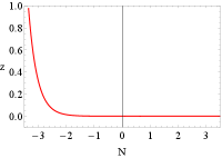
Now, we turn to study the evolution of the system with N. To solve the EOMs of this system, we take the initial condition to satisfy the current observation constrain, i.e., Eqs. (25) and (26). Besides, we assume that $z$ is small at the current universe. The evolutions of $x$ , $y$ and $z$ as the function of $N$ are shown in FIG.1. The red curves are for LQC and the blue dashed curves for the standard FRW cosmology. Notice that the parameters $\lambda$ and $\delta$ are chosen as $\lambda=2$ and $\delta=4.05$ , which satisfy the stability condition (28).

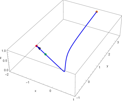
From this figure, we find that for most of the time of the universe evolution, $x$ and $y$ in LQC are the same as that in the standard FRW cosmology. Only in the early epoch of the universe, $x$ rapidly decreases and $y$ increases as time turns back. On the other hand, $z$ almost vanishes for most of the time of the universe evolution. But as time turns back, it rapidly increases in the early epoch of the universe. These phenomena indicate that LQG effect plays an important role only in the early epoch of the universe. Also, we show the parameter plot of $x$ , $y$ and $z$ in FIG.2. Indeed, the universe finally evolutes into the stability attractor solution (point C, red point in FIG.2).

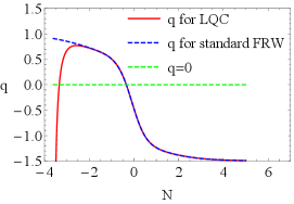
Further we plot the evolutions of the deceleration parameter $q$ with $N$ (FIG.3). We see that in the early epoch, the universe undergoes a so-called super-inflation stage due to the LQG effect Fu:2008gh ; Trojanowski:2020xza ; Pongkitivanichkul:2020txi ; Pacif:2020hai . After that, the universe enters into a decelerated phase, which is almost the same as that for the standard FRW cosmology. And then, the universe changes from this decelerated phase to an accelerated expansion stage where the LQG effect is diluted.

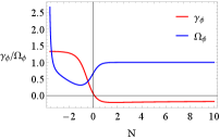
In FIG.4, we show the evolution of $\gamma_{\phi}$ and $\Omega_{\phi}$ with $N$ in the standard FRW cosmology (left) and LQC (right), respectively. Again, LQC effect plays a key role only in the early universe and is diluted as the time evolutes. Finally, the universe evolves into the stable attractor with $\gamma_{\phi}=0$ and $\Omega_{\phi}=1$ , which means the universe enters into a scalar field dominated one.

Finally, we would like to point out that the fixed points A and B are not stable fixed points but are the saddle ones because there are at least one negative eigenvalue for them (see TABLE 1).

III.2 K-essence with nonzero potential

Table 2: Fixed points for k-essence with non-zero potential

Point	x	y	b	Eigenvalues	$\Omega_{\phi}$	$\gamma_{\phi}$	Stability condition
A	0	$-\frac{\sigma}{12}$	$\frac{4+\sigma}{4}$	$\frac{1}{2}(-\delta+2\lambda-\sigma)$ , $\sigma$ , $-\sigma-3$ , $-4-\sigma$	1	${-\frac{\sigma}{3}}$	$2\lambda<\delta+\sigma$ and $\sigma>-3$
B	$-\frac{\sigma}{6}$	0	$\frac{6+\sigma}{6}$	$\sigma$ , $-3-\sigma$ , $-6-\sigma$ , $\delta-2\lambda+\sigma$	1	${-\frac{\sigma}{3}}$	$2\lambda>\delta+\sigma$ and $\sigma>-3$
C	$\frac{1}{2}(\delta-2(2+\lambda))$	$\frac{1}{6}(6-\delta+2\lambda)$	0	$-\delta+2\lambda$ , $\frac{\lambda^{2}-2\delta(5+2\lambda)+4(6+5\lambda+\lambda^{2})}{\delta-2(4+\lambda)}$ , $\delta-2\lambda-3$ , $\delta-2\lambda+\sigma$	1	${\frac{\delta-2\lambda}{3}}$	$2\lambda>\delta+\sigma$ and $\sigma>-3$
D	1	0	0	-4,1, $\frac{1}{2}(4-\delta+2\lambda)$ , $4+\sigma$	1	${\frac{4}{3}}$	unstable
E	0	$\frac{1}{3}$	0	-6,3, $\delta-6-2\lambda$ , $6+\sigma$	1	1	unstable

In this subsection, we study the dynamics of k-essence with nonzero potential. $V(\phi)\neq 0$ leads to $b\neq 0$ and so the dimension of this dynamical system becomes a $4$ -dimensional one. Then the scalar field fractional energy density $\Omega_{\phi}$ and the EOS parameter $\gamma_{\phi}$ become

	$\displaystyle\Omega_{\phi}=x+3y+b\,,\$		(29)
	$\displaystyle\gamma_{\phi}=\frac{2x+4y}{3+3y+b}\,.$		(30)

The values of $\Omega_{\phi}$ and $\gamma_{\phi}$ of the current universe (Eqs. (25) and (26)) gives the initial condition space as

	$\displaystyle x+3y+b=0.68\,,\$		(31)
	$\displaystyle 2x+4y=0.034\,.$		(32)

Given the initial condition, we can determine the evolutions of $x$ , $y$ , $z$ and $b$ with $N$ . Notice that the initial condition space is the same as that in the standard FRW cosmology. For the detailed discussions, please refer to Chakraborty:2019swx .

Following the same procedure above, we work out the fixed points and the stability conditions, which are shown in TABLE 2. From this table, we can see that the points D and E are the unstable points. We do not discuss these unstable points.

If the condition $2\lambda<\lambda+\sigma$ with $\sigma>-3$ is satisfied, A is a stable fixed point. We show the evolutions flowing to the fixed point A in FIG. 5. Here we have fixed $\sigma=0$ , which corresponds to the case of $\omega_{\phi}=-1$ ²²2For $\sigma<0$ , we have similar results. Notice that we do not consider the case of $\sigma>0$ , which cross the phantom field divide.. Regardless of the LQC or the standard FRW universe, the systems flow to the same fixed point $A$ . We note that as the time evolves, the linear and quadratic kinetic energy terms $x$ and $y$ reduce to zero, but the potential term $b$ increases and tends to the maximum value of $b=1$ . It suggests that as the quintessence dark energy model, the potential plays the dominant role in driving the cosmic acceleration in the later epoch of the universe. It is different from that for the pure k-essence, for which the kinetic energy terms play the role of driving the cosmic acceleration. As the case of pure k-essence studied above, only in the early stage of the universe, the LQG effects play an important role. In most of the evolution time of the universe, the evolution of the system in LQC are basically consistent with that in the standard FRW cosmology Ito:2012 ; Lin:2020fue ; LQGRovelli ; Guo:2003eu .

The corresponding $q$ , and $\gamma_{\phi}$ / $\Omega_{\phi}$ are also shown in FIG. 6 and FIG. 7, respectively. From the two figures, we can see that the LQG effect plays an import role in the early epoch of the universe such that the universe undergoes a super-inflation stage. And then, the LQG effect is diluted and the evolution of the universe is almost the same as that in the standard FRW universe. Finally, the universe flows to the scalar field dominated one.

When $2\lambda>\delta+\sigma$ with $\sigma>-3$ , the universe can flow to different fixed points $B$ and $C$ depending on the initial conditions. When the initial condition $x_{0}$ belongs to the region $x_{0}>0$ , the universe flows to the fixed point B, which is a potential energy dominant case (see FIG. 8). If $x_{0}<0$ , then the universe shall evolve into the fixed point C that a kinetic energy dominant case (see FIG. 9). And then, we also plot the evolutions of the deceleration parameter $q$ with $N$ for the initial conditions $x_{0}>0$ and $x_{0}<0$ in FIG. 10, respectively. We find that for the different initial conditions, the evolutions of the deceleration parameter $q$ are qualitatively consistent. That is to say, due to the LQG effect, the universe firstly undergoes a super-inflation stage. Soon afterwards, the universe enters into a decelerated phase and finally under the driving of scalar field, it enters into the accelerated expansion stage.

IV Dynamically changing $\lambda$ and $\delta$

In the previous section, $\lambda$ and $\delta$ are constant. Next, we study the evolution of the system with dynamically changing $\lambda$ and $\delta$ . We shall mainly study the case of pure k-essence. For the k-essence with nonzero potential, we only present a brief discussion.

The system of the pure k-essence with dynamically changing $\lambda$ and $\delta$ is a $5$ -dimensional system. Following the same procedure above, we can work out the fixed points and the corresponding eigenvalues, the parameters $\Omega_{\phi}$ and $\gamma_{\phi}$ in TABLE 3. The stability conditions are also summarized in this table.

Table 3: Fixed points for pure k-essence with dynamically changing

\lambda

and

\delta

Point	x	y	$\lambda$	$\delta$	$\Omega_{\phi}$	$\gamma_{\phi}$	Eigenvalues	Stability Condition
A	0	$\frac{1}{3}$	0	0	1	$\frac{4}{3}$	${-4,2,1,1,1}$	Unstable
B	0	$\frac{1}{3}$	0	$\frac{4}{5-4\tau}$	1	$\frac{4}{3}$	$\frac{4(-1+\tau)}{-5+4\tau}$ , $\frac{8(-1+\tau)}{-5+4\tau}$ ,-4,-1,1	Unstable
C	0	$\frac{1}{3}$	$\frac{1}{1-\Gamma}$	0	1	$\frac{4}{3}$	-4,-1,1,1, $\frac{-3+2\Gamma}{-1+\Gamma}$	Unstable
D	0	$\frac{1}{3}$	$\frac{4(-1+\tau)}{(-1+\Gamma)(-5+4\tau)}$	$\frac{4}{5-4\tau}$	1	$\frac{4}{3}$	$-\frac{4(-1+\tau)}{-5+4\tau}$ , $\frac{4(-3+2\Gamma)(-1+\tau)}{(-1+\Gamma)(-5+4\tau)}$ ,-4,-1,1	Unstable
E	-2	1	0	0	1	0	-3,-3,0,0,0	Saddle point
F	1	0	0	0	1	2	-6,-6,3,0,0	Unstable

Except the fixed point E, all fixed points are unstable because there is at least one positive eigenvalue for these fixed points. Since there are two negative eigenvalues and three zero eigenvalues for the fixed point E, it is a saddle point. These results for LQC are similar to the ones for the standard FRW universeLQGRovelli ; LQGThiemann ; Mulryne:2006cz .

We want to know the properties of the saddle point E. To this end, we show the evolutions of the system, the parameters $\Omega_{\phi}$ , $\gamma_{\phi}$ and $q$ with N for different $\Gamma$ and $\tau$ (FIG. 11, 12 and 13). The properties are summarized as what follows.

•

When $\Gamma$ and $\tau$ is small, the system flows to the fixed point E at the later stage (the first plot in FIG. 11). Correspondingly, $\Omega_{\phi}\rightarrow 1$ and $\gamma_{\phi}\rightarrow 0$ , which are the corresponding values of the fixed point E (see TABLE 3).
•

As $\Gamma$ and $\tau$ increase, some of the variables no longer flow to the fixe point E at the later stage (the second plot in FIG. 11). Some of the variables even become divergent at the later stage when $\Gamma$ and $\tau$ further increase (the third plot in FIG. 11). Correspondingly, $\gamma_{\phi}$ begins to deviate from the value of $\gamma_{\phi}=0$ for $\Gamma=\tau=1.4$ (the second plot in FIG. 12) and even divergent when $\Gamma$ and $\tau$ further increase to the value of $\Gamma=\tau=1.6$ (the third plot in FIG. 12).
•

The deceleration parameters $q$ is different for different $\Gamma$ and $\tau$ at the later stage. In particular, when $\Gamma=\tau=1.6$ , $q$ tends to divergent at later stage (FIG. 13).
•

Again, the LQG effect plays a key role only at the early stage.

To sum up, the saddle point E is not an attractor. Whether or not the system flows to this fixed point, it depends on the value of $\Gamma$ and $\tau$ .

The most general case is the one with nonzero potential and dynamically changing $\lambda$ and $\delta$ . In this case, the system is a $6$ -dimensional one. The fixed points and the corresponding eigenvalues are worked out in TABLE 4. There are $9$ fixed points for this system. But there are only two stable fixed points (C and D) and two saddle points (E and J) when the parameters satisfy certain conditions. Comparing with the case of the pure k-essence, the system possesses two stable fixed points under certain conditions such that we can model the evolution of the universe.

Table 4: Fixed points for k-essence with nonzero potential and dynamically changing

\lambda

and

\delta

Point

\lambda

\delta

Eigenvalues

Stability Condition

-\frac{\sigma}{12}

\frac{4+\sigma}{4}

-\frac{\sigma}{2}

-\frac{\sigma}{4}

\frac{\sigma}{4}

\sigma

-3-\sigma

-4-\sigma

Unstable

-\frac{\sigma}{12}

\frac{4+\sigma}{4}

\frac{\sigma}{4(-1+\Gamma)}

-\frac{\sigma}{4}

\frac{\sigma}{4}

-\frac{(-3+2\Gamma)\sigma}{4(-1+\Gamma)}

-3-\sigma

-4-\sigma

Unstable

-\frac{\sigma}{12}

\frac{4+\sigma}{4}

\frac{\sigma}{-5+4\tau}

-\frac{\sigma}{4}

\frac{\sigma}{4}

-3-\sigma

-4-\sigma

-\frac{2(-\sigma+\sigma\tau)}{-5+4\tau}

-\frac{-\sigma+\sigma\tau}{-5+4\tau}

-3<\sigma<0

1<\tau<5/4

-\frac{\sigma}{12}

\frac{4+\sigma}{4}

\frac{\sigma(-1+\tau)}{(-1+\Gamma)(-5+4\tau)}

\frac{\sigma}{-5+4\tau}

\frac{\sigma}{4}

\sigma

-3-\sigma

-4-\sigma

\frac{-\sigma+\sigma\tau}{-5+4\tau}

-\frac{(2\Gamma-3)(\tau-1)\sigma}{(-1+\Gamma)(-5+4\tau)}

\tau>5/4

\tau<1

1<\Gamma<3/2

-3<\sigma<0

-\frac{\sigma}{6}

\frac{6+\sigma}{6}

0,0,

\sigma

\sigma

-3-\sigma

-6-\sigma

Saddle point for

-3\leq\sigma\leq 0

\frac{1}{3}

-4,2,1,1,1,

4+\sigma

Unstable

\frac{1}{3}

\frac{4}{5-4\tau}

\frac{4(-1+\tau)}{-5+4\tau}

\frac{8(-1+\tau)}{-5+4\tau}

,-4,-1,1,

4+\sigma

Unstable

\frac{1}{3}

\frac{1}{1-\Gamma}

-4,-1,1,1,

\frac{-3+2\Gamma}{-1+\Gamma}

4+\sigma

Unstable

\frac{1}{3}

-\frac{4(-1+\tau)}{(-1+\Gamma)(-5+4\tau)}

\frac{4}{5-4\tau}

-\frac{4(-1+\tau)}{-5+4\tau}

\frac{4(-3+2\Gamma)(-1+\tau)}{(-1+\Gamma)(-5+4\tau)}

,-4,-1,1,

4+\sigma

Unstable

-2

-3,-3,0,0,0,

\sigma

Saddle point for

\sigma\leq 0

{-6,-6,3,0,0,6+\sigma}

Unstable

V Conclusion and discussion

In this paper, we have studied the dynamics of a k-essence in LQC. We in particular discuss the stability conditions of the fixed points. Comparing with the standard FRW universe, we need an additional dimensionless variable $z\equiv\rho_{t}/\rho_{c}$ . Notice that nonzero $z$ relates the LQG effect. Our discussion are divided into two main parts. One is that $\lambda$ and $\delta$ are treated as constant coupling parameters. Another is that $\lambda$ and $\delta$ are dynamically changing variables. For every case, we explore the dynamics of the pure k-essence and k-essence with nonzero potential, respectively. We summarize the main properties of the dynamical system as what follows.

•

$z$ is zero for all fixed point. It means that the LQG effect is diluted at the later stage of the universe. The evolution picture of the system indicates that LQG effect plays a key role only in the early epoch of the universe.
•

The fixed points in LQC are basically consistent with that in standard FRW cosmology Chakraborty:2019swx . For most of the attractor solutions, the stability conditions are consistent with that for the standard FRW universe. But for some special fixed point, for example, the fixed point C in TABLE 1, more tighter constraints are imposed thanks to the LQG effect.

In LQC framwork, there are several directions deserving further pursuit.

•

LQG effect is more evident in the early universe than the current universe. So it is interesting to study the evolution of k-essence in the early universe in LQC framework.
•

We can explore the k-essence dynamical system in spatially curved FRW universe Li:2010eua .
•

It is definitely interesting to study the dynamical system when an interaction term between k-essence and the fluid is included.
•

One of important dark energy models, different from the scalar field driving ones, is the so-called Chaplygin gap, which unifies the dark energy and dark matter Kamenshchik:2001cp ; Bento:2004uh ; Zhang:2005jj . Its dynamical behavior has also been studied in Li:2008uv . It is interesting to extend such studies to the LQC framework such that we can explore the effect of LQG.
•

It would be more interesting to study the dark energy evolution in the version of modified Friedmann equation proposed in Ding:2008tq ; Yang:2009fp . The version of modified Friedmann equation in Ding:2008tq ; Yang:2009fp reduces to the leading order effective one (Eq. (2)) if the higher correction term are neglected. The higher correction term may result in a qualitatively different scenario from that of the leading order effective theory (2).

Acknowledgements.

This work is supported by the Natural Science Foundation of China under Grant Nos. 11775036, and Fok Ying Tung Education Foundation under Grant No.171006. Jian-Pin Wu is also supported by Top Talent Support Program from Yangzhou University.

References

(1) A. G. Riess et al. [Supernova Search Team], “Observational evidence from supernovae for an accelerating universe and a cosmological constant,” Astron. J. 116 (1998), 1009-1038 [arXiv:astro-ph/9805201 [astro-ph]].
(2) S. Perlmutter et al. [Supernova Cosmology Project], “Measurements of $\Omega$ and $\Lambda$ from 42 high redshift supernovae,” Astrophys. J. 517 (1999), 565-586 [arXiv:astro-ph/9812133 [astro-ph]].
(3) C. L. Bennett et al. [WMAP], Astrophys. J. Suppl. 148 (2003), 1-27 [arXiv:astro-ph/0302207 [astro-ph]].
(4) D. N. Spergel et al. [WMAP], “First year Wilkinson Microwave Anisotropy Probe (WMAP) observations: Determination of cosmological parameters,” Astrophys. J. Suppl. 148 (2003), 175-194 [arXiv:astro-ph/0302209 [astro-ph]].
(5) M. Tegmark et al. [SDSS], “Cosmological parameters from SDSS and WMAP,” Phys. Rev. D 69 (2004), 103501 [arXiv:astro-ph/0310723 [astro-ph]].
(6) M. Tegmark et al. [SDSS], “The 3-D power spectrum of galaxies from the SDSS,” Astrophys. J. 606 (2004), 702-740 [arXiv:astro-ph/0310725 [astro-ph]].
(7) C. Armendariz-Picon, T. Damour and V. F. Mukhanov, “k - inflation,” Phys. Lett. B 458 (1999), 209-218 [arXiv:hep-th/9904075 [hep-th]].
(8) J. Garriga and V. F. Mukhanov, “Perturbations in k-inflation,” Phys. Lett. B 458 (1999), 219-225 [arXiv:hep-th/9904176 [hep-th]].
(9) T. Chiba, T. Okabe and M. Yamaguchi, “Kinetically driven quintessence,” Phys. Rev. D 62 (2000), 023511 [arXiv:astro-ph/9912463 [astro-ph]].
(10) C. Armendariz-Picon, V. F. Mukhanov and P. J. Steinhardt, “A Dynamical solution to the problem of a small cosmological constant and late time cosmic acceleration,” Phys. Rev. Lett. 85 (2000), 4438-4441 [arXiv:astro-ph/0004134 [astro-ph]].
(11) C. Armendariz-Picon, V. F. Mukhanov and P. J. Steinhardt, “Essentials of k essence,” Phys. Rev. D 63 (2001), 103510 [arXiv:astro-ph/0006373 [astro-ph]].
(12) S. Tsujikawa, “General analytic formulae for attractor solutions of scalar-field dark energy models and their multi-field generalizations,” Phys. Rev. D 73 (2006), 103504 [arXiv:hep-th/0601178 [hep-th]].
(13) Y. Gong, A. Wang and Y. Z. Zhang, “Exact scaling solutions and fixed points for general scalar field,” Phys. Lett. B 636 (2006), 286-292 [arXiv:gr-qc/0603050 [gr-qc]].
(14) P. G. Ferreira and M. Joyce, “Cosmology with a primordial scaling field,” Phys. Rev. D 58 (1998), 023503 [arXiv:astro-ph/9711102 [astro-ph]].
(15) E. J. Copeland, A. R. Liddle and D. Wands, “Exponential potentials and cosmological scaling solutions,” Phys. Rev. D 57 (1998), 4686-4690 [arXiv:gr-qc/9711068 [gr-qc]].
(16) Z. K. Guo, Y. S. Piao, R. G. Cai and Y. Z. Zhang, “Cosmological scaling solutions and cross coupling exponential potential,” Phys. Lett. B 576 (2003), 12-17 [arXiv:hep-th/0306245 [hep-th]].
(17) Z. K. Guo, Y. S. Piao and Y. Z. Zhang, “Cosmological scaling solutions and multiple exponential potentials,” Phys. Lett. B 568 (2003), 1-7 [arXiv:hep-th/0304048 [hep-th]].
(18) K. Lin and W. L. Qian, “Cosmic evolution of dark energy in a generalized Rastall gravity,” Eur. Phys. J. C 80 (2020) no.6, 561 [arXiv:2006.03229 [gr-qc]].
(19) E. J. Copeland, M. Sami and S. Tsujikawa, “Dynamics of dark energy,” Int. J. Mod. Phys. D 15 (2006), 1753-1936 [arXiv:hep-th/0603057 [hep-th]].
(20) L. A. Urena-Lopez, “Scalar phantom energy as a cosmological dynamical system,” JCAP 09 (2005), 013 [arXiv:astro-ph/0507350 [astro-ph]].
(21) J. Carot and M. M. Collinge, “Scalar field cosmologies: A Dynamical systems study,” Class. Quant. Grav. 20 (2003), 707-728
(22) Y. Ito, S. Nojiri and S.D. Odintsov, “Stability of Accelerating Cosmology in Two Scalar-Tensor Theory: Little Rip versus de Sitter,” Entropy, 14, 1578 (2012).
(23) C. Rovelli, Quantum Gravity, (Cambridge University Press, 2004).
(24) T. Thiemann, Modern Canonical Quantum General Relativity, (Cambridge University Press, 2007).
(25) A. Ashtekar and J. Lewandowski, “Background independent quantum gravity: A Status report,” Class. Quant. Grav. 21 (2004), R53 [arXiv:gr-qc/0404018 [gr-qc]].
(26) M. Han, W. Huang and Y. Ma, “Fundamental structure of loop quantum gravity,” Int. J. Mod. Phys. D 16 (2007), 1397-1474 [arXiv:gr-qc/0509064 [gr-qc]].
(27) M. Bojowald, “Absence of singularity in loop quantum cosmology,” Phys. Rev. Lett. 86 (2001), 5227-5230 [arXiv:gr-qc/0102069 [gr-qc]].
(28) A. Ashtekar, T. Pawlowski and P. Singh, “Quantum nature of the big bang,” Phys. Rev. Lett. 96 (2006), 141301 [arXiv:gr-qc/0602086 [gr-qc]].
(29) A. Ashtekar, T. Pawlowski and P. Singh, “Quantum Nature of the Big Bang: Improved dynamics,” Phys. Rev. D 74 (2006), 084003 [arXiv:gr-qc/0607039 [gr-qc]].
(30) M. Bojowald, “Loop quantum cosmology,” Living Rev. Rel. 8 (2005), 11 [arXiv:gr-qc/0601085 [gr-qc]].
(31) A. Ashtekar, M. Bojowald and J. Lewandowski, “Mathematical structure of loop quantum cosmology,” Adv. Theor. Math. Phys. 7 (2003) no.2, 233-268 [arXiv:gr-qc/0304074 [gr-qc]].
(32) A. Ashtekar and P. Singh, “Loop Quantum Cosmology: A Status Report,” Class. Quant. Grav. 28 (2011), 213001 [arXiv:1108.0893 [gr-qc]].
(33) A. Ashtekar, T. Pawlowski and P. Singh, “Quantum Nature of the Big Bang: An Analytical and Numerical Investigation. I.,” Phys. Rev. D 73 (2006), 124038 [arXiv:gr-qc/0604013 [gr-qc]].
(34) M. Bojowald, G. Date and K. Vandersloot, “Homogeneous loop quantum cosmology: The Role of the spin connection,” Class. Quant. Grav. 21 (2004), 1253-1278 [arXiv:gr-qc/0311004 [gr-qc]].
(35) P. Singh and A. Toporensky, “Big crunch avoidance in K=1 semiclassical loop quantum cosmology,” Phys. Rev. D 69 (2004), 104008 [arXiv:gr-qc/0312110 [gr-qc]].
(36) G. V. Vereshchagin, “Qualitative approach to semi-classical loop quantum cosmology,” JCAP 07 (2004), 013 [arXiv:gr-qc/0406108 [gr-qc]].
(37) G. Date, “Absence of the Kasner singularity in the effective dynamics from loop quantum cosmology,” Phys. Rev. D 71 (2005), 127502 [arXiv:gr-qc/0505002 [gr-qc]].
(38) G. Date and G. M. Hossain, “Genericity of big bounce in isotropic loop quantum cosmology,” Phys. Rev. Lett. 94 (2005), 011302 [arXiv:gr-qc/0407074 [gr-qc]].
(39) R. Goswami, P. S. Joshi and P. Singh, “Quantum evaporation of a naked singularity,” Phys. Rev. Lett. 96 (2006), 031302 [arXiv:gr-qc/0506129 [gr-qc]].
(40) M. Bojowald, “The Early universe in loop quantum cosmology,” J. Phys. Conf. Ser. 24 (2005), 77-86 [arXiv:gr-qc/0503020 [gr-qc]].
(41) T. Stachowiak and M. Szydlowski, “Exact solutions in bouncing cosmology,” Phys. Lett. B 646 (2007), 209-214 [arXiv:gr-qc/0610121 [gr-qc]].
(42) M. Bojowald, “Inflation from quantum geometry,” Phys. Rev. Lett. 89 (2002), 261301 [arXiv:gr-qc/0206054 [gr-qc]].
(43) E. J. Copeland, D. J. Mulryne, N. J. Nunes and M. Shaeri, “Super-inflation in Loop Quantum Cosmology,” Phys. Rev. D 77 (2008), 023510 [arXiv:0708.1261 [gr-qc]].
(44) M. Bojowald, H. H. Hernandez, M. Kagan, P. Singh and A. Skirzewski, “Hamiltonian cosmological perturbation theory with loop quantum gravity corrections,” Phys. Rev. D 74 (2006), 123512 [arXiv:gr-qc/0609057 [gr-qc]].
(45) M. Bojowald, H. Hernandez, M. Kagan, P. Singh and A. Skirzewski, “Formation and Evolution of Structure in Loop Cosmology,” Phys. Rev. Lett. 98 (2007), 031301 [arXiv:astro-ph/0611685 [astro-ph]].
(46) M. Bojowald, G. M. Hossain, M. Kagan and S. Shankaranarayanan, “Anomaly freedom in perturbative loop quantum gravity,” Phys. Rev. D 78 (2008), 063547 [arXiv:0806.3929 [gr-qc]].
(47) M. Bojowald and G. M. Hossain, “Cosmological vector modes and quantum gravity effects,” Class. Quant. Grav. 24 (2007), 4801-4816 [arXiv:0709.0872 [gr-qc]].
(48) M. Bojowald and G. M. Hossain, “Loop quantum gravity corrections to gravitational wave dispersion,” Phys. Rev. D 77 (2008), 023508 [arXiv:0709.2365 [gr-qc]].
(49) J. P. Wu and Y. Ling, “The Cosmological perturbation theory in loop cosmology with holonomy corrections,” JCAP 05 (2010), 026 [arXiv:1001.1227 [hep-th]].
(50) J. P. Wu and Y. Ma, “Anomaly freedom of the vector modes with holonomy corrections in perturbative Euclidean loop quantum gravity,” Phys. Rev. D 86 (2012), 124044 [arXiv:1209.2766 [gr-qc]].
(51) J. P. Wu, M. Bojowald and Y. Ma, “Anomaly freedom in perturbative models of Euclidean loop quantum gravity,” Phys. Rev. D 98 (2018) no.10, 106009 [arXiv:1809.04465 [gr-qc]].
(52) G. M. Hossain, “Primordial density perturbation in effective loop quantum cosmology,” Class. Quant. Grav. 22 (2005), 2511-2532 [arXiv:gr-qc/0411012 [gr-qc]].
(53) G. Calcagni and M. Cortes, “Inflationary scalar spectrum in loop quantum cosmology,” Class. Quant. Grav. 24 (2007), 829-854 [arXiv:gr-qc/0607059 [gr-qc]].
(54) D. J. Mulryne and N. J. Nunes, “Constraints on a scale invariant power spectrum from superinflation in LQC,” Phys. Rev. D 74 (2006), 083507 [arXiv:astro-ph/0607037 [astro-ph]].
(55) X. Zhang and Y. Ling, “Inflationary universe in loop quantum cosmology,” JCAP 08 (2007), 012 [arXiv:0705.2656 [gr-qc]].
(56) M. Artymowski, Z. Lalak and L. Szulc, “Loop Quantum Cosmology: holonomy corrections to inflationary models,” JCAP 01 (2009), 004 [arXiv:0807.0160 [gr-qc]].
(57) S. Tsujikawa, P. Singh and R. Maartens, “Loop quantum gravity effects on inflation and the CMB,” Class. Quant. Grav. 21 (2004), 5767-5775 [arXiv:astro-ph/0311015 [astro-ph]].
(58) M. Shimano and T. Harada, “Observational constraints on a power spectrum from super-inflation in Loop Quantum Cosmology,” Phys. Rev. D 80 (2009), 063538 [arXiv:0909.0334 [gr-qc]].
(59) Y. Ding, Y. Ma and J. Yang, “Effective Scenario of Loop Quantum Cosmology,” Phys. Rev. Lett. 102 (2009), 051301 [arXiv:0808.0990 [gr-qc]].
(60) H. Wei and S. N. Zhang, “Dynamics of Quintom and Hessence Energies in Loop Quantum Cosmology,” Phys. Rev. D 76 (2007), 063005 [arXiv:0705.4002 [gr-qc]].
(61) P. Wu and S. N. Zhang, “Cosmological evolution of interacting phantom (quintessence) model in Loop Quantum Gravity,” JCAP 06 (2008), 007 [arXiv:0805.2255 [astro-ph]].
(62) X. Fu, H. W. Yu and P. Wu, “Dynamics of interacting phantom scalar field dark energy in Loop Quantum Cosmology,” Phys. Rev. D 78 (2008), 063001 [arXiv:0808.1382 [gr-qc]].
(63) S. Chen, B. Wang and J. Jing, “Dynamics of interacting dark energy model in Einstein and Loop Quantum Cosmology,” Phys. Rev. D 78 (2008), 123503 [arXiv:0808.3482 [gr-qc]].
(64) H. Zonunmawia, W. Khyllep, N. Roy, J. Dutta and N. Tamanini, “Extended Phase Space Analysis of Interacting Dark Energy Models in Loop Quantum Cosmology,” Phys. Rev. D 96 (2017) no.8, 083527 [arXiv:1708.07716 [gr-qc]].
(65) S. Li and Y. Ma, “Dark Energy Interacting with Dark Matter in Classical Einstein and Loop Quantum Cosmology,” Eur. Phys. J. C 68 (2010), 227-239 [arXiv:1004.4350 [astro-ph.CO]].
(66) A. Chakraborty, A. Ghosh and N. Banerjee, “Dynamical systems analysis of a k -essence model,” Phys. Rev. D 99 (2019) no.10, 103513 [arXiv:1904.10149 [gr-qc]].
(67) J. Yang, Y. Ding and Y. Ma, “Alternative quantization of the Hamiltonian in loop quantum cosmology II: Including the Lorentz term,” Phys. Lett. B 682 (2009), 1-7 [arXiv:0904.4379 [gr-qc]].
(68) M. Assanioussi, A. Dapor, K. Liegener and T. Pawłowski, “Emergent de Sitter Epoch of the Quantum Cosmos from Loop Quantum Cosmology,” Phys. Rev. Lett. 121 (2018) no.8, 081303 [arXiv:1801.00768 [gr-qc]].
(69) S. Bahamonde, C. G. Böhmer, S. Carloni, E. J. Copeland, W. Fang and N. Tamanini, “Dynamical systems applied to cosmology: dark energy and modified gravity,” Phys. Rept. 775-777 (2018), 1-122 [arXiv:1712.03107 [gr-qc]].
(70) B. Gumjudpai, T. Naskar, M. Sami and S. Tsujikawa, “Coupled dark energy: Towards a general description of the dynamics,” JCAP 06 (2005), 007 [arXiv:hep-th/0502191 [hep-th]].
(71) Caldwell, Robert and Kamionkowski, Marc and Weinberg, Nevin, Phys.Rev.Lett 91 (2003) no.10.071301
(72) S. Trojanowski, P. Brax and C. van de Bruck, “Dark matter relic density from conformally or disformally coupled light scalars,” Phys. Rev. D 102 (2020) no.2, 023035 [arXiv:2006.01149 [hep-ph]].
(73) C. Pongkitivanichkul, D. Samart, N. Thongyoi and N. Lunrasri, “A Kaluza-Klein Inspired Brans-Dicke Gravity with Dark Matter and Dark Energy Model,” [arXiv:2005.08791 [gr-qc]].
(74) S. K. J. Pacif, “Dark energy models from a parametrization of $H$ : A comprehensive analysis and observational constraints,” [arXiv:2005.06972 [physics.gen-ph]].
(75) J. L. Li and J. P. Wu, “Dynamics of tachyon field in spatially curved FRW universe,” Phys. Lett. B 686 (2010), 221-226 [arXiv:1003.1870 [hep-th]].
(76) A. Y. Kamenshchik, U. Moschella and V. Pasquier, “An Alternative to quintessence,” Phys. Lett. B 511 (2001), 265-268 [arXiv:gr-qc/0103004 [gr-qc]].
(77) M. C. Bento, O. Bertolami and A. A. Sen, “The Revival of the unified dark energy - dark matter model?,” Phys. Rev. D 70 (2004), 083519 [arXiv:astro-ph/0407239 [astro-ph]].
(78) H. S. Zhang and Z. H. Zhu, “Interacting chaplygin gas,” Phys. Rev. D 73 (2006), 043518 [arXiv:astro-ph/0509895 [astro-ph]].
(79) S. Li, Y. Ma and Y. Chen, “Dynamical Evolution of Interacting Modified Chaplygin Gas,” Int. J. Mod. Phys. D 18 (2009), 1785-1800 [arXiv:0809.0617 [gr-qc]].

Dynamics of k-essence in loop quantum cosmology

Abstract

I Introduction

II K-essence in LQC

III Dynamics with constant coupling parameters

III.1 Pure k-essence

III.2 K-essence with nonzero potential

IV Dynamically changing λ\lambda and δ\delta

V Conclusion and discussion

Acknowledgements.

References

IV Dynamically changing $\lambda$ and $\delta$