Dynamics of ferromagnetic bimerons driven by spin currents and magnetic fields
Abstract
Magnetic bimeron composed of two merons is a topological counterpart of magnetic skyrmion in in-plane magnets, which can be used as the nonvolatile information carrier in spintronic devices. Here we analytically and numerically study the dynamics of ferromagnetic bimerons driven by spin currents and magnetic fields. Numerical simulations demonstrate that two bimerons with opposite signs of topological numbers can be created simultaneously in a ferromagnetic thin film via current-induced spin torques. The current-induced spin torques can also drive the bimeron and its speed is analytically derived, which agrees with the numerical results. Since the bimerons with opposite topological numbers can coexist and have opposite drift directions, two-lane racetracks can be built in order to accurately encode the data bits. In addition, the dynamics of bimerons induced by magnetic field gradients and alternating magnetic fields are investigated. It is found that the bimeron driven by alternating magnetic fields can propagate along a certain direction. Moreover, combining a suitable magnetic field gradient, the Magnus-force-induced transverse motion can be completely suppressed, which implies that there is no skyrmion Hall effect. Our results are useful for understanding of the bimeron dynamics and may provide guidelines for building future bimeron-based spintronic devices.
pacs:
75.10.Hk, 75.70.Kw, 75.78.-n, 12.39.DcI Introduction
Topologically nontrivial magnetic skyrmions have received a lot of attention, because they have small size and low depinning current, and can be used as information carriers for information storage and computing applications Roszler_NATURE2006 ; Nagaosa_NNANO2013 ; Finocchio_JPD2016 ; Kang_PIEEE2016 ; Fert_NATREVMAT2017 ; ES_JAP2018 ; Zhou_NSR2018 ; Zhang_SciRep2015 ; Prychynenko_PRApplied2018 ; Nozaki_APL2019 ; Zhang_JPCM2020 ; Bogdanov_1989 . Magnetic skyrmions have been experimentally observed in systems with bulk or interfacial Dzyaloshinskii-Moriya interaction (DMI) Nagaosa_NNANO2013 ; Finocchio_JPD2016 ; Fert_NATREVMAT2017 ; ES_JAP2018 , and can be manipulated by various methods, such as electric currents Sampaio_NatNano2013 ; Iwasaki_NatNano2013 ; Zhang_PRB2016 , spin waves Zhang_Nanotech2015 , magnetic field gradients Komineas_PRB2015 ; Wang_NJP2017 ; Liang_NJP2018 , magnetic anisotropy gradients Wang_Nanoscale2018 ; Xia_JMMM2018 ; Tomasello_PRB2018 ; Shen_PRB2018 ; Ma_NanoLett2019 and temperature gradients Kong_PRL2013 ; Khoshlahni_PRB2019 . In addition, various topologically nontrivial spin textures, such as antiferromagnetic skyrmions Zhang_SREP2016A ; Barker_PRL2016 ; Yang_PRL2018 ; Shen_APL2019 ; Liang_PRB2019 , ferrimagnetic skyrmions Woo_NATCOM2018 , antiskyrmions Nayak_Nature2017 , and bimerons Ezawa_PRB2011 ; Zhang_SciRep2015 ; Lin_PRB2015 ; Heo_SciRep2016 ; Leonov_PRB2017 ; Kharkov_PRL2017 ; Kolesnikov_SciRep2018 ; Chmiel_NatMater2018 ; Yu_Nat2018 ; Woo_Nat2018 ; Gobel_PRB2019 ; Fernandes_SSC2019 ; Murooka2019 ; Kim2019 ; Moon_arX2018 ; Shen_PRL2020 ; Lu_arXiv2020 ; Zarzuela_PRB2020 ; Zhang_Bimeron2020 ; Li_arXiv2020 , are also currently hot topics.
Particularly, a bimeron composed of two merons can be regarded as a counterpart of the skyrmion in in-plane magnets, which can be attained by rotating the spin texture of a skyrmion by . Gobel_PRB2019 Therefore, the ferromagnetic (FM) bimerons share the characteristics of skyrmions, such as small size and topologically nontrivial spin structure, and they also show the transverse drift during force-driven motion, i.e., the skyrmion Hall effect Jiang_NatPhys2017 ; Litzius_NatPhys2017 . The skyrmion Hall effect may cause the skyrmion (or bimeron) to annihilate at the sample edge, which is detrimental for practical applications. To overcome or suppress the skyrmion Hall effect, various ways have been proposed, such as adopting synthetic antiferromagnetic skyrmions Zhang_NATCOM2016 ; Xia_PRApplied2019 ; Legrand_NatMat2019 ; Dohi_NATCOM2019 or applying high magnetic anisotropy in the racetrack edge Lai_SciRep2017 . Magnetic bimerons, which can be found in various magnets Kharkov_PRL2017 ; Zhang_Bimeron2020 ; Zhang_SciRep2015 ; Lin_PRB2015 ; Leonov_PRB2017 ; Murooka2019 ; Zarzuela_PRB2020 ; Shen_PRL2020 ; Li_arXiv2020 ; Gobel_PRB2019 , also has the potential to be used as information carriers for spintronic devices made of in-plane magnetized thin films Zhang_SciRep2015 ; Gobel_PRB2019 ; Murooka2019 . Recent studies on bimerons Gobel_PRB2019 ; Murooka2019 ; Shen_PRL2020 ; Moon_arX2018 ; Zarzuela_PRB2020 ; Zhang_Bimeron2020 ; Li_arXiv2020 focus on its dynamics induced by electric currents. However, an electric current faces the issue of Joule heating and is not applicable for insulating materials. Therefore, it is necessary to explore alternative methods for manipulating FM bimerons effectively.
In this work, we report the dynamics of FM bimerons induced by spin currents and magnetic fields. We numerically realize the simultaneous creation of two bimerons with opposite topological numbers via current-induced spin torques, and we theoretically prove that such two bimerons can coexist in a FM film with interfacial DMI. Our results show that in addition to the spin current, a magnetic field gradient can drive a FM bimeron to motion. Furthermore, excited by alternating magnetic field, the bimeron propagates along a certain direction, which does not show the skyrmion Hall effect when a suitable magnetic field gradient is further adopted.
II Model and simulation
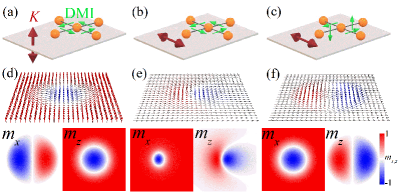
Considering a FM film with perpendicular magnetic anisotropy [Fig. 1(a)], the skyrmion [Fig. 1(d)] can be stabilized by introducing the isotropic interfacial DMI Tomasello_SciRep2014 ; Rohart_PRB2013 , where the DMI can be induced at the ferromagnet/heavy metal (such as Ta and Pt) interface. Here we focus on the study of a FM film with in-plane easy-axis anisotropy [Fig. 1(b)]. In such a FM system, the asymmetrical bimeron [Fig. 1(e)] is formed when the isotropic interfacial DMI is adopted. We employ the Landau-Lifshitz-Gilbert (LLG) equation Gilbert_IEEE2004 with the damping-like spin torque to simulate the dynamics of FM systems, which is described as
| (1) |
( with saturation magnetization ) is the reduced magnetization and denotes the partial derivative of the magnetization with respect to time. The damping-like spin torque can be produced by injecting a current into a magnetic tunnel junction or using the spin Hall effect. is the polarization vector and relates to the applied current density , defined as with the reduced Planck constant , the spin Hall angle , the vacuum permeability constant , the elementary charge , and the layer thickness . and denote the gyromagnetic ratio and the damping constant respectively. stands for the effective field obtained from the variation of the FM energy ,
| (2) | ||||
where the first, second, third and fourth terms represent the exchange energy, magnetic anisotropy energy, Zeeman energy and DMI energy respectively. In Eq. (2), , and are the exchange constant, magnetic anisotropy constant and DMI constant respectively. stands for the direction of the anisotropy axis, and is the applied magnetic field. Note that the thermal fluctuation and dipole-dipole interaction are not taken into account.
To obtain the bimeron mentioned above, the presence of in-plane magnetic anisotropy in materials (such as CoFeB Kipgen_JMMM2012 ) is essential. On the other hand, the out-of-plane spin configurations exist in the bimeron, and they will increase the system energy if the in-plane anisotropy is considered. By introducing other energies, such as the DMI energy, which lends to spin canting, the energy increase due to the anisotropy can be compensated, so that the bimeron can be formed in a FM film with DMI and in-plane easy-axis anisotropy (the stability diagram of the bimeron is shown in Fig. S1 of Ref. Shen_SI ). Similar to DMI, the frustrated exchange interaction can also bring the spin canting Gobel_PRB2019 , so that the bimeron can be stabilized in frustrated FM systems Zhang_Bimeron2020 . In addition to ferromagnets, the bimeron is a stable solution in antiferromagnets in the presence of DMI and in-plane anisotropy Shen_PRL2020 ; Li_arXiv2020 . Note that the shape of bimerons depends on the DMI. Taking isotropic DMI (see Fig. 1), i.e., the DMI vectors are in-plane and DMI energy constant , the formed bimeron has asymmetrical shape Li_arXiv2020 . If we rotate the DMI vectors by [see Fig. 1(c)] Gobel_PRB2019 , the bimeron shape will be symmetrical [see Fig. 1(f)] Shen_PRL2020 . The dynamics of symmetrical and asymmetrical FM bimerons induced by alternating magnetic fields will be discussed later, while for the bimeron in antiferromagnet, it is difficult to excite its dynamics by a magnetic field.
III Spin current-induced creation of bimerons
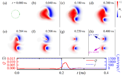
Creating bimerons is the foundation for their practical applications. Here we use a spin current to create the bimerons via damping-like spin torques. As shown in Fig. 2(a), the initial state is the FM ground state. When the current pulse of MA/cm2 and is injected into the central circular region with diameter of 30 nm, the magnetization in the circular region will be flipped towards the direction of the polarization vector , as shown in Fig. 2(b). At ns [Fig. 2(d)], the current is switched off, and then the magnetic texture is relaxed [see Figs. 2(e)-(h)]. Figure 2(h) shows that after the relaxation, two bimerons are simultaneously generated. In addition, we calculate the time evolution of the topological number Barker_PRL2016 ; Lin_PRB2015 ; Tretiakov_PRB2007 , showing that for the two bimerons created here, the sum of their topological numbers equals to zero [see Fig. 2(i)]. This indicates their opposite topological numbers, which is also confirmed in Fig. 2(h). A pair of bimerons with opposite shown in Fig. 2(h) can be separated into two independent bimerons when a suitable spin current is applied, as they have opposite drift directions (see Fig. 4). Note that an isolated bimeron with positive will be created when MA/cm2, as shown in Fig. S2 of Ref. Shen_SI . If the sign of current is changed, i.e., MA/cm2, the created bimeron has negative .
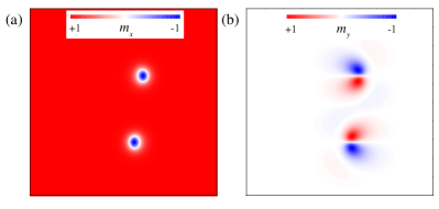
In order to analyze such a phenomenon, i.e., two bimerons with opposite signs of are stabilized in a FM film with the same background (see Supplementary Movie 1), Moon_arX2018 ; Murooka2019 we present the components and of the magnetization for the case of Fig. 2(h), as shown in Fig. 3. Figures 2(h) and 3 suggest that by using the operation , two bimerons created here can convert to each other. On the other hand, the operation mentioned above will affect the spatial derivative of the magnetization, . Thus, we obtain the operation for the spatial derivative of the magnetization, and . Taking the above operation and combining Eq. (2), it is found that the system energy is not changed, however giving rise to a change in the sign of the topological number . As a result, the bimerons with opposite signs of can coexist in the FM film with in-plane anisotropy and isotropic DMI (see Fig. 1), while in a FM system with perpendicular magnetic anisotropy and isotropic DMI, the coexistence of different skyrmions with opposite topological numbers is not allowed. We note that taking the same values of parameters, the asymmetrical bimerons have a smaller size compared to the skyrmions.
IV spin current-driven motion of bimerons
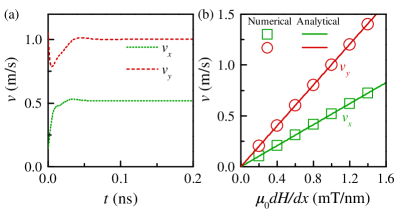
In addition to creating the bimerons, manipulating them is also indispensable for the application of information storage and logic devices. We now use the spin current (instead of electric current) to manipulate the bimerons. Taking the current density MA/cm2 and the damping , the time evolution of the velocities (, ) for bimerons with opposite signs of is shown in Figs. 4(a)-(f), where the velocity and the guiding center (, ) of the bimeron is defined as Komineas_PRB2015
| (3) |
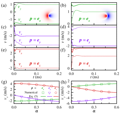
From Fig. 4, we can see that for the cases where the polarization vector and , the bimerons can be driven to motion and the velocity reaches a constant value at ns. For the bimerons with opposite signs of , a spin current drives them to drift in the opposite directions. Namely, their skyrmion Hall angles [] have opposite signs. The above result means that two-lane racetracks (or double-bit racetracks) can be built in order to accurately encode the data bits, where the presence of a bimeron in the top and bottom lanes is used to encode the data bits “1” and “0” respectively. Moon_arX2018 ; Muller_NJP2017 ; Kang_IEDL2016 ; Lai_Spin2017 Compared to the single-lane racetrack based on skyrmions, such a two-lane racetrack based on bimerons is robust for the data representation, as we always detect a bimeron for the data bits “1” and “0”. In the single-lane racetrack, the data bits “1” and “0” are encoded by the presence and absence of a skyrmion respectively. However, the distance between two skyrmions may be affected by many factors, so that the number of the data bit “0” cannot be accurately encoded by the absence of a skyrmion.
By changing the damping constant , the different values of the velocities (, ) are obtained from the numerical simulations, as shown in Figs. 4(g) and (h). In order to test the reliability of the simulated speeds, from Eq. (1), we derive the steady motion equation for the FM bimeron using Thiele’s (or collective coordinate) approach Thiele_PRL1973 ; Tveten_PRL2013 ; Tretiakov_PRL2008 ; Clarke_PRB2008 , written as
| (4) |
where is the gyrovector. represents the dissipative force with the dissipative tensor , where the component of the dissipative tensor is . denotes the driving force, which is described as with when the damping-like spin torque is considered. From Eq. (4), we obtain the steady motion speed,
| (5) |
where , and has been used Shen_SI . Figures 4(g) and (h) show that the analytical results given by Eq. (5) are in good agreement with the numerical simulations. Note that for the case of (along the anisotropy axis), asymmetrical bimerons can be driven, while for a symmetrical bimeron, is derived so that its motion speed is equal to zero.
V Motion of bimerons driven by magnetic field gradients
Using the magnetic field as a driving source is applicable in both metals and insulating materials, so it is an important manipulation method, and it is necessary to discuss the dynamics of bimeron induced by magnetic fields. In the next sections, we focus on the study of the bimeron dynamics induced by magnetic field gradients and alternating magnetic fields. Figure 5(a) shows the time evolution of the velocities (, ) for the bimeron with positive , where a magnetic field gradient ( with mT/nm, where the gradient value could be feasible in experiments Jakobi_NatNano2017 ) is applied and the damping . For the case shown in Fig. 5(a), the change of bimeron size induced by the magnetic field can be ignored, and the velocities (, ) at ns almost reach a constant value of (0.518 m/s, 1.002 m/s). Figure 5(b) shows that the velocities of the bimeron are proportional to the magnetic field gradient. Due to the presence of the magnetic field gradient, the potential energy of the system changes spatially, so that a nonzero driving force will act on the FM bimeron. We now derive the formula of the driving force induced by the magnetic field with a constant gradient. Applying a partial integration, Komineas_PRB2015 the induced force is derived from , which is described as
| (6) |
where is 94.4 nm2 for the parameters used here Shen_SI . Substituting the above Eq. (6) into Eq. (5), we obtain the steady motion speed, and find that the bimeron moves towards the area of lower magnetic field, similar to the case of the skyrmion Wang_NJP2017 . As shown in Fig. 5(b), the results given by Eqs. (5) and (6) are consistent with the numerical simulations.
VI Motion of bimerons driven by alternating magnetic fields
Recently, an interesting method for manipulating magnetic skyrmions, was proposed, i.e., by using an oscillating electric field and combining a static magnetic field, where the electric field can modify the magnetic anisotropy. Yuan_PRB2019 ; Song_JPD2019 Such a method is applicable in both metals and insulators. With the oscillating electric field alone, the skyrmion will exhibit the breathing motion (rather than propagation along a certain direction) and the spin wave excitation is symmetric. When an in-plane static magnetic field is applied, the symmetry of the skyrmion is broken and then the spin wave excitation becomes asymmetric, resulting in nonzero net driving force. Yuan_PRB2019 ; Song_JPD2019 Thus, an oscillating electric field can drive the asymmetrical skyrmion to move along a certain direction. In addition, the skyrmion speed reaches its maximum value when the frequency of the oscillating electric field matches the eigenfrequency of the system. Yuan_PRB2019
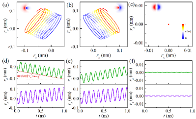
The bimerons studied here have intrinsic asymmetrical structure, so that they can be driven by the alternating field. Figures 6(a) and (b) show the trajectories of asymmetrical bimerons driven by an alternating magnetic field sin(), where the applied magnetic field is uniform in space. Indeed, the propagation of asymmetrical bimerons is induced, and for the bimerons with opposite signs of , their trajectories are essentially the same, except for their motion directions. For the purpose of comparison, we also calculate the motion of the symmetrical bimeron under the same magnetic field, as shown in Fig. 6(c), from which we can see that an alternating magnetic field cannot induce the symmetrical bimeron to propagation. Note that in addition to the alternating magnetic field, the alternating magnetic anisotropy can also excite the asymmetrical bimeron to move along a certain direction, as shown in Fig. S5 of Ref. Shen_SI .
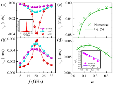
On the other hand, based on the time evolution of the guiding center (, ), the propagation velocities (, ) of the bimeron can be obtained [see Fig. 6(d)]. Figures 7(a) and (b) show the velocities as functions of the frequency , where we take the alternating magnetic field sin() with amplitude of 10 mT and frequency of GHz. Similar to the case of the skyrmion, Yuan_PRB2019 the bimeron reaches its maximum speed when the frequency of alternating magnetic fields coincides with the system eigenfrequency of GHz [see the inset in Fig. 7(a)]. In addition, the velocities (, ) are calculated as functions of the damping , as shown in Figs. 7(c) and (d), where the alternating magnetic field has the amplitude of 10 mT and frequency of 20 GHz. To understand the results of the numerical simulations, we try to find the net driving force induced by the alternating magnetic field. As shown in the inset of Fig. 7(d), the ratio obtained from numerical simulations can be described by . Thus, Eq. (5) suggests that the net driving force is almost along the direction. Assuming that with N, N, N and N, the results given by Eq. (5) agree with the numerical simulations, as shown in Figs. 7(c) and (d). It is worth mentioning that the bimeron will annihilate, when a strong alternating magnetic field (its amplitude and frequency are 100 mT and 20 GHz respectively) is applied (see Supplementary Movie 2).
VII Magnetic bimerons showing no skyrmion Hall effect
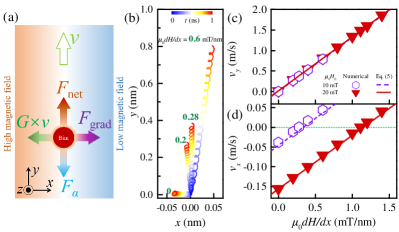
As shown in Figs. 6 and 7, under the action of the alternating magnetic field, the FM bimerons show the skyrmion Hall effect due to the presence of the Magnus force (), and the motion speed is small ( m/s). Here we introduce a force induced by magnetic field gradients to compensate the Magnus force, and then achieve this purpose of overcoming or suppressing the skyrmion Hall effect, as shown in Fig. 8(a), where the direction of the net driving force (the direction) is parallel to the racetrack. Figure 8(b) shows that as the magnetic field gradient increases, the bimeron moves faster and the skyrmion Hall effect is effectively suppressed. When increases to 0.28 mT/nm, the bimeron propagates parallel to the racetrack with the speed of m/s, so that the bimeron will not be destroyed by touching the racetrack edge. On the other hand, for the case of 0.28 mT/nm, the propagation of the bimeron is perpendicular to the gradient direction, so that the bimeron size is not affected by the space-dependent magnetic field. If 0.28 mT/nm, the force induced by the magnetic field gradient is larger than the Magnus force (), causing that the bimeron moves towards the area of lower magnetic field [see Fig. 8(b)].
By changing the magnetic field gradient , the different velocities are obtained by numerical simulations, as shown in Figs. 8(c) and (d). In our simulations, the damping 0.1, the frequency of alternating magnetic fields is 20 GHz, and the amplitudes of 10 and 20 mT are adopted. Combining the Eq. (6) and substituting into Eq. (5), the analytical velocities are given. As shown in Figs. 8(c) and (d), the results given by Eq. (5) are consistent with numerical simulations, where the values of and N have been used for the cases of 10 and 20 mT respectively. We now derive the critical magnetic field gradient, at which the bimeron moves without showing the skyrmion Hall effect, i.e., . Based on , the critical magnetic field gradient is derived, which satisfies the following formula,
| (7) |
where . As mentioned earlier, for the case of 10 mT, our numerical simulation shows that the critical magnetic field gradient is 0.28 mT/nm and the corresponding speed is 0.374 m/s. If the amplitude of the alternating magnetic field is increased to 20 mT, the critical magnetic field gradient and corresponding speed are 1.11 mT/nm and 1.486 m/s, respectively, as shown in Figs. 8(c) and (d). The above values obtained from numerical simulations obey Eq. (7).
VIII Conclusions
In conclusion, we analytically and numerically study the dynamics of FM bimerons induced by spin currents and magnetic fields. Numerical simulations show that two bimerons with opposite signs of the topological numbers can be simultaneously created in a FM film via current-induced spin torques, and we prove their energy equivalence. However, the coexistence of two skyrmions with opposite topological numbers is not allowed in a FM film with the same background. Compared to the skyrmions, the bimerons studied here have a smaller size for the same values of parameters. The motion of bimerons induced by spin currents is also discussed, and the bimeron speed is analytically derived, which agrees well with the numerical simulations. We point out that two-lane racetracks based on bimerons can be built in order to accurately encode the data bits, as the bimerons with opposite topological numbers can coexist and have opposite drift directions. In addition, a magnetic field gradient can drive a bimeron towards the area of lower magnetic field. More importantly, when only an alternating magnetic field is applied to the entire film system, the asymmetrical bimeron propagates along a certain direction. Besides, if a suitable magnetic field gradient is further introduced, the alternating magnetic field can drive the bimeron to move at a speed of 1.5 m/s and the bimeron does not show the skyrmion Hall effect. Our results are useful for understanding of the bimeron dynamics and may provide effective ways for building bimeron-based spintronic devices.
Acknowledgements.
X.L. acknowledges the support by the Guangdong Basic and Applied Basic Research Foundation (Grant No. 2019A1515111110). X.Z. acknowledges the support by the Guangdong Basic and Applied Basic Research Foundation (Grant No. 2019A1515110713), and the Presidential Postdoctoral Fellowship of The Chinese University of Hong Kong, Shenzhen (CUHKSZ). O.A.T. acknowledges the support by the Australian Research Council (Grant No. DP200101027) and the Cooperative Research Project Program at the Research Institute of Electrical Communication, Tohoku University. M.E. acknowledges the support by the Grants-in-Aid for Scientific Research from JSPS KAKENHI (Grant Nos. JP18H03676 and JP17K05490) and the support by CREST, JST (Grant Nos. JPMJCR16F1 and JPMJCR1874). Y.Z. acknowledges the support by the President’s Fund of CUHKSZ, Longgang Key Laboratory of Applied Spintronics, National Natural Science Foundation of China (Grant Nos. 11974298 and 61961136006), Shenzhen Fundamental Research Fund (Grant No. JCYJ20170410171958839), Shenzhen Key Laboratory Project (Grant No. ZDSYS201603311644527), and Shenzhen Peacock Group Plan (Grant No. KQTD20180413181702403).References
- (1) A. N. Bogdanov and D. A. Yablonskii, Sov. Phys. JETP 68, 101 (1989).
- (2) U. K. Rößler, A. N. Bogdanov, and C. Pfleiderer, Nature 442, 797 (2006).
- (3) N. Nagaosa and Y. Tokura, Nat. Nanotechnol. 8, 899 (2013).
- (4) G. Finocchio, F Büttner, R. Tomasello, M. Carpentieri and M. Kläui, J. Phys. D: Appl. Phys. 49, 423001 (2016).
- (5) A. Fert, N. Reyren and V. Cros, Nat. Rev. Mat. 2, 17031 (2017).
- (6) K. Everschor-Sitte, J. Masell, R. M. Reeve, and M. Kläui, J. Appl. Phys. 124, 240901 (2018).
- (7) W. Kang, Y. Huang, X. Zhang, Y. Zhou, and W. Zhao, Proc. IEEE 104, 2040 (2016).
- (8) Y. Zhou, Natl. Sci. Rev. 6, 210 (2019).
- (9) X. Zhang, Y. Zhou, K. M. Song, T.-E. Park, J. Xia, M. Ezawa, X. Liu, W. Zhao, G. Zhao, and S. Woo, J. Phys. Condens. Matter 32, 143001 (2020).
- (10) X. Zhang, M. Ezawa, and Y. Zhou, Sci. Rep. 5, 9400 (2015).
- (11) D. Prychynenko, M. Sitte, K. Litzius, B. Krüger, G. Bourianoff, M. Kläui, J. Sinova, and K. Everschor-Sitte, Phys. Rev. Appl. 9, 014034 (2018).
- (12) T. Nozaki, Y. Jibiki, M. Goto, E. Tamura, T. Nozaki, H. Kubota, A. Fukushima, S. Yuasa, and Y. Suzuki, Appl. Phys. Lett. 114, 012402 (2019).
- (13) J. Sampaio, V. Cros, S. Rohart, A. Thiaville, and A. Fert, Nat. Nanotechnol. 8, 839 (2013).
- (14) J. Iwasaki, M. Mochizuki, and N. Nagaosa, Nat. Nanotechnol. 8, 742 (2013).
- (15) X. Zhang, Y. Zhou, and M. Ezawa, Phys. Rev. B 93, 024415 (2016).
- (16) X. Zhang, M. Ezawa, D. Xiao, G. P. Zhao, Y. Liu, and Y. Zhou, Nanotechnology 26, 225701 (2015).
- (17) S. Komineas and N. Papanicolaou, Phys. Rev. B 92, 064412 (2015).
- (18) C. Wang, D. Xiao, X. Chen, Y. Zhou, and Y. Liu, New J. Phys. 19, 083008 (2017).
- (19) J. J. Liang, J. H. Yu, J. Chen, M. H. Qin, M. Zeng, X. B. Lu, X. S. Gao, and J.-M. Liu, New J. Phys. 20, 053037 (2018).
- (20) X. Wang, W. L. Gan, J. C. Martinez, F. N. Tan, M. B. A. Jalil, and W. S. Lew, Nanoscale 10, 733 (2018).
- (21) H. Xia, C. Song, C. Jin, J. Wang, J. Wang, and Q. Liu, J. Magn. Magn. Mater. 458, 57 (2018).
- (22) R. Tomasello, S. Komineas, G. Siracusano, M. Carpentieri, and G. Finocchio, Phys. Rev. B 98, 024421 (2018).
- (23) L. Shen, J. Xia, G. Zhao, X. Zhang, M. Ezawa, O. A. Tretiakov, X. Liu, and Y. Zhou, Phys. Rev. B 98, 134448 (2018).
- (24) C. Ma, X. Zhang, J. Xia, M. Ezawa, W. Jiang, T. Ono, S. N. Piramanayagam, A. Morisako, Y. Zhou, and X. Liu, Nano Lett. 19, 353 (2019).
- (25) L. Kong and J. Zang, Phys. Rev. Lett. 111, 067203 (2013).
- (26) R. Khoshlahni, A. Qaiumzadeh, A. Bergman, and A. Brataas, Phys. Rev. B 99, 054423 (2019).
- (27) X. Zhang, Y. Zhou, and M. Ezawa, Sci. Rep. 6, 24795 (2016).
- (28) J. Barker and O. A. Tretiakov, Phys. Rev. Lett. 116, 147203 (2016).
- (29) H. Yang, C. Wang, T. Yu, Y. Cao, and P. Yan, Phys. Rev. Lett. 121, 197201 (2018).
- (30) L. Shen, J. Xia, G. Zhao, X. Zhang, M. Ezawa, O. A. Tretiakov, X. Liu, and Y. Zhou, Appl. Phys. Lett. 114, 042402 (2019).
- (31) X. Liang, G. Zhao, L. Shen, J. Xia, L. Zhao, X. Zhang, and Y. Zhou, Phys. Rev. B 100, 144439 (2019).
- (32) S. Woo, K. M. Song, X. Zhang, Y. Zhou, M. Ezawa, X. Liu, S. Finizio, J. Raabe, N. J. Lee, S. I. Kim, S. Y. Park, Y. Kim, J. Y. Kim, D. Lee, O. Lee, J. W. Choi, B. C. Min, H. C. Koo, and J. Chang, Nat. Commun. 9, 959 (2018).
- (33) A. K. Nayak, V. Kumar, T. Ma, P. Werner, E. Pippel, R. Sahoo, F. Damay, U. K. Rößler, C. Felser, and S. S. P. Parkin, Nature 548, 561 (2017).
- (34) M. Ezawa, Phys. Rev. B 83, 100408(R) (2011).
- (35) S. Z. Lin, A. Saxena, and C. D. Batista, Phys. Rev. B 91, 224407 (2015).
- (36) C. Heo, N. S. Kiselev, A. K. Nandy, S. Blügel, and T. Rasing, Sci. Rep. 6, 27146 (2016).
- (37) A. O. Leonov and I. Kézsmárki, Phys. Rev. B 96, 014423 (2017).
- (38) Y. A. Kharkov, O. P. Sushkov, and M. Mostovoy, Phys. Rev. Lett. 119, 207201 (2017).
- (39) A. G. Kolesnikov, V. S. Plotnikov, E. V. Pustovalov, A. S. Samardak, L. A. Chebotkevich, A. V. Ognev, and O. A. Tretiakov, Sci. Rep. 8, 15794 (2018).
- (40) F. P. Chmiel, N. Waterfield Price, R. D. Johnson, A. D. Lamirand, J. Schad, G. van der Laan, D. T. Harris, J. Irwin, M. S. Rzchowski, C. B. Eom, and P. G. Radaelli, Nat. Mater. 17, 581 (2018).
- (41) X. Z. Yu, W. Koshibae, Y. Tokunaga, K. Shibata, Y. Taguchi, N. Nagaosa, and Y. Tokura, Nature 564, 95 (2018).
- (42) S. Woo, Nature 564, 43 (2018).
- (43) B. Göbel, A. Mook, J. Henk, I. Mertig, and O. A. Tretiakov, Phys. Rev. B 99, 060407(R) (2019).
- (44) R. L. Fernandes, R. J. C. Lopes, and A. R. Pereira, Solid State Commun. 290, 55 (2019).
- (45) R. Murooka, A. O. Leonov, K. Inoue and J. Ohe, Sci. Rep. 10, 396 (2020).
- (46) S. K. Kim, Phys. Rev. B 99, 224406 (2019).
- (47) K.-W. Moon, J. Yoon, C. Kim, and C. Hwang, Phys. Rev. Appl. 12, 064054 (2019).
- (48) L. Shen, J. Xia, X. Zhang, M. Ezawa, O. A. Tretiakov, X. Liu, G. Zhao, and Y. Zhou, Phys. Rev. Lett. 124, 037202 (2020).
- (49) X. Zhang, J. Xia, L. Shen, M. Ezawa, O. A. Tretiakov, G. Zhao, X. Liu, and Y. Zhou, Phys. Rev. B 101, 144435 (2020).
- (50) R. Zarzuela, V. K. Bharadwaj, K.-W. Kim, J. Sinova, and K. Everschor-Sitte, Phys. Rev. B 101, 054405 (2020).
- (51) X. Lu, R. Fei, and L. Yang, arXiv:2002.05208 (2020).
- (52) X. Li, L. Shen, Y. Bai, X. Zhang, J. Xia, M. Ezawa, O. A. Tretiakov, X. Xu, M. Mruczkiewicz, M. Krawczyk, and Y. Zhou, arXiv:2002.04387 (2020).
- (53) W. Jiang, X. Zhang, G. Yu, W. Zhang, X. Wang, M. Benjamin Jungfleisch, John E. Pearson, X. Cheng, O. Heinonen, K. L. Wang, Y. Zhou, A. Hoffmann, and Suzanne G. E. te Velthuis, Nat. Phys. 13, 162 (2017).
- (54) K. Litzius, I. Lemesh, B. Krüger, P. Bassirian, L. Caretta, K. Richter, F. Büttner, K. Sato, O. A. Tretiakov, J. Förster, R. M. Reeve, M. Weigand, I. Bykova, H. Stoll, G. Schütz, G. S. D. Beach, and M. Kläui, Nat. Phys. 13, 170 (2017).
- (55) X. Zhang, Y. Zhou, and M. Ezawa, Nat. Commun. 7, 10293 (2016).
- (56) J. Xia, X. Zhang, M. Ezawa, Z. Hou, W. Wang, X. Liu, and Y. Zhou, Phys. Rev. Appl. 11, 044046 (2019).
- (57) W. Legrand, D. Maccariello, F. Ajejas, S. Collin, A. Vecchiola, K. Bouzehouane, N. Reyren, V. Cros, and A. Fert, Nat. Mater. 19, 34 (2019).
- (58) T. Dohi, S. DuttaGupta, S. Fukami, and H. Ohno, Nat. Commun. 10, 5153 (2019).
- (59) P. Lai, G. P. Zhao, H. Tang, N. Ran, S. Q. Wu, J. Xia, X. Zhang, and Y. Zhou, Sci. Rep. 7, 45330 (2017).
- (60) R. Tomasello, E. Martinez, R. Zivieri, L. Torres, M. Carpentieri, and G. Finocchio, Sci. Rep. 4, 6784 (2014).
- (61) S. Rohart and A. Thiaville, Phys. Rev. B 88, 184422 (2013).
- (62) L. Kipgen, H. Fulara, M. Raju, and S. Chaudhary, J. Magn. Magn. Mater. 324, 3118, (2012).
- (63) See Supplemental Material at http:// for the detailed results on the FM bimerons.
- (64) T. L. Gilbert, IEEE Trans. Magn. 40, 3443 (2004).
- (65) O. A. Tretiakov and O. Tchernyshyov, Phys. Rev. B 75, 012408 (2007).
- (66) J. Müller, New J. Phys. 19, 025002 (2017).
- (67) W. Kang, C. Zheng, Y. Huang, X. Zhang, Y. Zhou, W. Lv and W. Zhao, IEEE Electron Devices Lett. 37, 924 (2016).
- (68) P. Lai, G. P. Zhao, F. J. Morvan, S. Q. Wu and N. Ran, Spin 7, 1740006 (2017).
- (69) A. A. Thiele, Phys. Rev. Lett. 30, 230 (1973).
- (70) E. G. Tveten, A. Qaiumzadeh, O. A. Tretiakov, and A. Brataas, Phys. Rev. Lett. 110, 127208 (2013).
- (71) O. A. Tretiakov, D. Clarke, G. W. Chern, Y. B. Bazaliy, and O. Tchernyshyov, Phys. Rev. Lett. 100, 127204 (2008).
- (72) D. J. Clarke, O. A. Tretiakov, G. W. Chern, Y. B. Bazaliy, and O. Tchernyshyov, Phys. Rev. B 78, 134412 (2008).
- (73) I. Jakobi, P. Neumann, Y. Wang, D. B. R. Dasari, F. E. Hallak, M. A. Bashir, M. Markham, A. Edmonds, D. Twitchen, and J. Wrachtrup, Nat. Nanotechnol. 12, 67 (2017).
- (74) H. Y. Yuan, X. S. Wang, M.-H. Yung, and X. R. Wang, Phys. Rev. B 99, 014428 (2019).
- (75) C. Song, C. Jin, Y. Ma, J. Wang, H. Xia, J. Wang, and Q. Liu, J. Phys. D: Appl. Phys. 52, 435001 (2019).