Dynamics of descending knots in a solar prominence and their possible contributions to the heating of the local corona
Abstract
The knots in solar prominences are often observed to fall with nearly constant velocity, but the associated physical mechanism is currently not well understood. In this letter, we presented a prominence observed by New Vacuum Solar Telescope (NVST) in wavelength. Knots that rose within the prominence appear to have been preferentially located at higher altitude, whereas those that fell were found throughout the entire prominence structure. The descending speed of the knots near the solar surface was higher than that far away from the solar surface. We noted that the knots near the solar surface may run along a set of coronal loops observed from the Atmospheric Imaging Assembly. Elsewhere, the majority of knots are interpreted to have descended across more horizontal magnetic field with a nearly constant speed. This lack of acceleration indicates that the liberated gravitational potential energy may not manifest as an increase in kinetic energy. Assuming instead that the descending knots were capable of exciting Alfvén waves that could then dissipate within the local corona, the gravitational potential energy of the knots may have been converted into thermal energy. Assuming a perfectly elastic system, we therefore estimate that the gravitational energy loss rate of these observed knots amounts to 1/2000 of that required to heat the entire quiet-Sun, increasing to 1/320 when considering possibly further downward motions of the knots having disappeared in the observations. This result suggests such a mechanism may contribute to the heating of the corona local to these prominences.
1 Introduction
Solar prominences are the plasma structures with high density and low temperature in the tenuous and hot corona (Labrosse et al., 2010; Mackay et al., 2010). The so-called hedgerow type prominence is the quiescent prominence that consists of long and tall blade-like palisades (Engvold, 2015). Observations have shown that the plasma within such prominences typically exhibit both vertical and horizontal flows of the order of tens of km s-1 (Engvold, 1976; Chae, 2010; Liu et al., 2012). Similar to the bidirectional pattern of flows found in a filament (Zirker et al., 1998), persistent horizontal flows that may reach long distances can be detected in hedgerow prominences (Chae et al., 2008). However, of particular interest are the thin, downward-directed mass flows with velocities much less than free-fall speeds. The observational study by Liu et al. (2012) led the authors to suggest that the entire mass of a prominence could be swapped out on the order of a day by these vertical flows. The mechanism responsible for then replenishing the drained prominence material has been suggested to be some form of coincident condensation process (e.g., Antiochos et al., 1999; Keppens et al., 2015; Xia & Keppens, 2016) or a consequence of the draining material interacting with the transition region via the Rayleigh Taylor instability (RTI) (see e.g., Keppens et al., 2015; Kaneko & Yokoyama, 2018). The RTI has also previously been invoked to explain the thin rising plumes that are typically coincident with the aforementioned falling structures (e.g., Hillier et al., 2012), not to be confused with the large voids that have been observed to grow beneath prominences and are believed to be associated with flux emergence (e.g., Berger et al., 2010).
The horizontal flows seen in the prominence are often interpreted as observational evidence that the plasma is supported by the sagging of initially horizontal magnetic field lines (Chae et al., 2008; Shen et al., 2015). As such, it remains an open question as to how the knots observed to fall may do so through a medium permeated by horizontal magnetic field. Low et al. (2012) suggested that a downward resistive flow across the supporting horizontal field is a result of developing of a mass sheet singularity under the falling knots, while Chae (2010) proposed instead that magnetic reconnection takes place around the descending knots. However, Haerendel & Berger (2011) suggested that the horizontal orientation of the external field is rather unfavorable for magnetic reconnection with the knots. Assuming that the plasma packet constituting the knots has a very high value of beta, the author suggested that the knots will behave like a diamagnetic body, which deforms the ambient field as it slips through it. The downward acceleration is then counterbalanced by a friction force due to dissipation of Alfvén waves along the horizontal magnetic field, and then the downward motions keep almost a constant speed.
If the falling knots travel with constant downward speed along more vertical magnetic field, a hydrostatic pressure gradient could provide an upward force which may balance the force of gravity acting on the falling knots. Modeling the evolution of a density enhancement in a stratified atmosphere with uniform magnetic field, Mackay & Galsgaard (2001) found that this pressure gradient can build up under the density enhancement, causing it to fall through the stratified atmosphere with speeds much less than the free-fall speed. Similarly, Oliver et al. (2014) investigated the dynamical evolution of a fully ionized plasma blob in an isothermal, vertically stratified corona. The authors found that the presence of a heavy condensation gave rise to the formation of a large pressure gradient that opposed gravity, and eventually this pressure gradient became so large that the blob acceleration vanishes. In the model proposed by Low et al. (2012), the liberated energy is converted to dissipative energy that fuels the radiative loss of the prominence plasma. By contrast, Haerendel & Berger (2011) suggested that the Alfvén waves excited by the falling knots carry away the liberated energy.
Coronal heating is a topic dedicated to explaining how the corona may be heated up to a temperature of millions of degrees, far above that of the photosphere. Alfvén-wave turbulence is a promising candidate to transport magneto-convective energy upwards along the Sun’s magnetic field lines into the corona. McIntosh et al. (2011) detected Alfvénic waves in type II spicules, which could be energetic enough to heat the quiet corona. Samanta et al. (2019) showed the evidence that these spicules may originate from the solar surface. However, some further investigations showed that the wave energy communicated by spicules was in actual fact far less than that required to heat the corona of the quiet-Sun (Thurgood et al., 2014; Weberg et al., 2018). As another candidate for heating the corona, the nanoflare proposal suggested by Parker (1988) involved the slow braiding of coronal field lines and the impulsive release of stored energy. Using high-resolution coronal imager instrument onboard a rocket, Cirtain et al. (2013) suggested the magnetic braids in a coronal active region that are reconnecting, relaxing and dissipating sufficient energy to heat the corona. However, the braiding and relaxation are not immediately obvious as noted by Zirker & Engvold (2017). The magnetic reconnection associated with the newly emergence flux may also contribute to heat the quiet Sun (Close et al., 2005; Zhang et al., 2015).
In this study, we have investigated the vertical motion of knots within a solar prominence observed using the New Vacuum Solar Telescope (Liu et al., 2001, 2014, NVST). We have identified the rising and descending knots in the presented prominence, before estimating the velocity and acceleration of the knots on the plane of sky. This allows us to investigate the spatial distribution of temporal kinetics of the knots. Furthermore, we have roughly estimated the loss rate of the gravitational potential from the descending knots and compared it with heating power requirement for the corona in the quiet Sun.
2 Observation and Data analysis
2.1 Overview of the observation
NVST is a ground-based multi-channel high resolution imaging system, including , G-band, TiO band and CaII 8542 Å wavelengths. The studied prominence, located on the west limb of the Sun, was observed by NVST from 02:20 to 07:10 UT on Jan 7, 2017. During this period, NVST provides the linecore image with prefilter width of 0.25 Å. These images have a temporal cadence of 11s, a spatial sampling of , and a field of view of . A high resolution NVST image is normally reconstructed from at least 100 short exposure images. After reconstruction (Xiang et al., 2016), the actual resolution of an image of the chromosphere (, 6563 Å) is better than . With such a spatial resolution, NVST can resolve many fundamental structures in the photosphere and chromosphere within a field of view (Xu et al., 2014).
The observed prominence in image has a length of Mm and an upper extent of Mm. Figure 1a presents an image that is aligned to the full-disk GONG image, which has a spatial sampling of .
The Atmospheric Imaging Assembly (AIA; Lemen et al., 2012) on board the Solar Dynamic Observatory (SDO; Pesnell et al., 2012) provides full-disk images of the corona with a spatial sampling of . Comparing the image with AIA/304 Å image (Figure 1c), we can see that the prominence observed in is the northern part of a larger prominence in 304 Å image.
As shown on the bottom panels in Figure 1, the images were rotated to ensue that the photospheric limb is horizontal. The AIA 211 Å image (Figure 1f) that is taken at the same time with the NVST image (Figure 1g) shows that a set of coronal loops appears under the prominence on the limb. Taken at an earlier time, the 211 Å image presents that the coronal arcades (denoted by the arrow in Figure 1e) seem to be located around one endpoint of the prominence (Figure 1e). Based on a high accuracy solar image registration procedure (Feng et al., 2012; Yang et al., 2014), all of the NVST images are aligned to the same FOV as indicated by Figure 1g. This will allow us to study the motions of the structures detected in the NVST images.
2.2 The technique of optical flow
Time sequences of high-cadence images enable the identification and study of the dynamics features across the image plane. The optical flow, referring to the proper motion of a feature across the image plane, may be used to determine the velocity field from two images. The technique of local correlation tracking (LCT; November, & Simon, 1988) and the differential affine velocity estimator (DAVE; Schuck, 2006) are two kinds of optical flow techniques that have been widely used in the solar research.
Thirion (1988) presented a model to perform image-to-image matching by determining the optical flow between two images. The author illustrated the concept of this model by an analogy with Maxwell’s demons, as such this algorithm is usually named as non-rigid Demon algorithm. Liu et al. (2018) have examined the performance of three different methods (Demon, DAVE, and LCT) using a photosphere and chromosphere image provided by NVST. After shifting the images 5.6 pixel in x direction and 0.2 pixel in y direction, they noted that the Demon found displacements are more close to the true displacements and then they suggested that the Demon algorithm outperforms traditional LCT and DAVE methods in estimating the analog displacements both smaller and bigger than one pixel.
Here, we used both the DAVE and Demon algorithms to obtain the optical flow between two NVST images. The earlier image is set as the reference image and and the later image as the target image. As an example, Figure 2a shows a reference image and Figure 2d shows the difference image between the reference and target image. The DAVE and Demon velocity fields are indicated by arrows on Figure 2b and 2c , respectively. To test the performance of each technique, we warped the reference image to align with the target image based on the resulted optical flow. Ideally, the warped image would be identical to the target image. Figure 2e (2f) presents the difference image between the target image and the warped image based on DAVE (Demon). Comparing the warping image based on DAVE, the Demon-based warping image has less difference from the target image. Based on these results, the Demon-based optical flow is chosen to study the velocity of the knots in the prominence. As shown in the Appendix, the errors of the velocities measured by Demon is about 2 km s-1.
2.3 Identifying and tracking knots
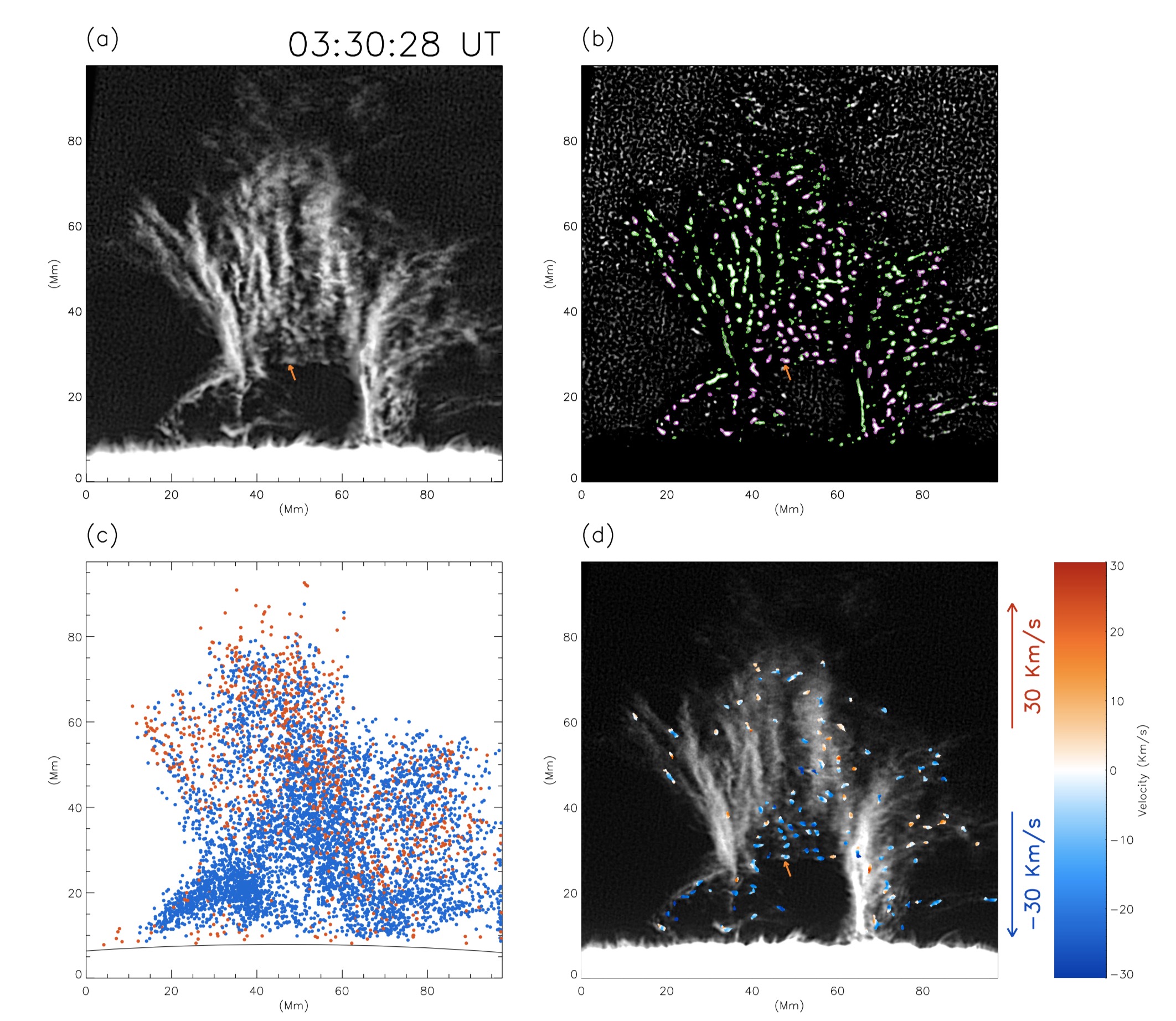
Different from the vertical thread in the prominence, the bright knots appear to be brighter and shorter in the vertical direction. Here, we used morphological approach to identify the rising or descending knots in the prominence. Firstly, since the bright knots are located on nonuniform background, contrast of the image was enhanced using contrast-limited adaptive histogram equalization (CLAHE; Zuiderveld, 1994). Figure 3a presents one of the enhanced images. A representative bright knot is denoted by the arrow in Figure 3a. Secondly, to further enhance contrast of the bright knots on the images, we performed morphological top-hat filtering on the enhanced image, the bright knots were then separated from the background (Figure 3b). Based on a threshold of intensity value on the top-hat transformed image, the bright knots can be identified, as the color ( magenta and green) contours outlined (Figure 3b). Third, to distinguish between the rising and falling blobs, and other uninteresting features, we selected the structures that have a vertical displacement larger than its initial vertical extent. As shown in Figure 3b, the magenta contours denote the rising or descending bright knots that are selected, while the uninteresting features are colored green. Each point in Figure 3c denotes the location where each knot starts to be identified. The knots with rising and descending motions are colored red and blue, respectively. It is obvious from the distribution of points that the rising knots are often located in the higher altitude, while the descending motions in the low altitude. In Figure 3d, the identified knots are colored based on the vertical velocity estimated from Demon.
3 Results
Applying the algorithm outlined above to the images, we identified and tracked 6194 moving bright knots. The widths of the knots range from 1 Mm to 3 Mm (Figure 4a). The heights of the knots to solar surface range from 2 – 85 Mm (Figure 4b). Among these tracked knots, 4655 knots show downward motions, and the remaining 1539 knots show upward motions. The knots travel upward or downward with a vertical distance of several Mm (Figure 4c). Figure 4c shows the distribution of the vertical distances that the knots traveled. Here, positive and negative value means that the knot has experienced a downward and upward motion, respectively. We found that the majority of knots disappeared from the image after rising or falling less than 4 Mm. These knots are visible in less than 10 images and their lifetimes range from 1 to 2 minutes. However, 713 of the 4655 downward knots were detected to travel longer than 4 Mm in the vertical direction, among which 75 knots descend more than 10 Mm.
The velocity of a knot is estimated by averaging the Demon velocities of the knot detected at different times. The histogram in Figure 4d shows the vertical velocity distribution for the identified knots. Again, more knots are found to display downward velocity. The descending knots fall at the speed of about 18 km s-1, while the other knots rise at the lower speed of 10 km s-1.
The acceleration of a knots is obtained by a least square linear fit for the velocity, such as , where is the vertical velocity of a knots observed in the ith moment. The histogram of (Figure 4e) shows that the distribution of knot acceleration peaks at a value of zero with a FWHM of only 0.42, where =0.272 km s-2 near the solar surface.
Figure 4g presents the histogram of the brightness of knots. Again, the brightness of a knot is defined as the average of that of the knot detected at different moments. We defined the change rate of the brightness of an identified knot as , where is a linear fit to the brightness of a knot detected at the ith image, i=1, 2, … N, and a knot is identified in N images. The greater than zero means that the total brightness increases when a knot rises or descends, while lower than zero indicates the brightness decreases. The histogram in Figure 4h shows that the distribution of is close to a gaussian profile with a peak at -0.10, indicating that the number of knots whose brightness decreases over time is slightly bigger.
It is worth noting that, however, the knots disappeared in the image after the knots were traced in several or more images. In order to isolate the final velocity and the brightness of the knots that were recognized in the images, we defined
| (1) |
where the term “end” denotes the image in which a knot was recognized at last time. The larger value of () indicates larger change in the vertical velocity (total brightness) of a knot before it disappears. The histogram of (Figure 4f) shows a gaussian profile with peak at -0.1, while the histogram of (Figure 4i) fits a Gaussian distribution with the peak at -0.39. Therefore, at a time when these knots were about to disappear on the image, the brightness of knots decreased impulsively but their descending velocity did not change significantly. It implies that the knots may keep falling after they cannot be identified in the images.
Figure 5a shows an averaged image, in which each pixel is an average of the brightness of the knots that are detected at the same location at different times. Similarly, Figure 5b and 5c shows the averaged Demon velocity distribution of the knots in the horizontal and vertical direction, respectively. Figure 5b shows that the horizontal velocity is close to 30 km s-1 on the bottom of the prominence and is greater than 5 km s-1 in most areas at higher altitude. In Figure 5c, the upward vertical velocity could be found predominantly in the upper portions of the prominence whereas the downward velocity were present at seemingly all altitudes with the strongest signatures at the bottom of the prominence.
To detail the value of the speed of the falling knots, Figure 5e shows the distribution of the vertical velocity in the downward direction. In the area denoted by the box in Figure 5e, the downward velocity of the knots is greater than 25 km s-1. Comparing to the FOV of AIA 211 Å , the box covers a set of coronal loops (Figure 5d). It is thus possible that the quickly falling knots may run along magnetic field that is marked by the coronal loops. The majority of knots outside the box were found to descend with a velocity lower than 25 km s-1. Overall, the largest downward velocities were located at the bottom of the prominence.
The acceleration of a knot was estimated from the result of linear fit to the vertical speed of an identified knot in three moments. The map in Figure 5f then presents averaged acceleration of the identified knots, in which the dashed-line denotes the height of 7 Mm above the solar surface. The majority of the knots at a height above 7 Mm appear to have had a downward acceleration much less than the gravitational acceleration experienced at the solar surface. However, within about 7 Mm above solar surface, the knots underwent a rapid deceleration, with the value of acceleration as high as .
4 Discussions
In this study,we have identified and tracked the knots within a solar prominence that was observed by the NVST. Although knots were observed to have propagated both upwards and downwards (with respect to the solar surface), a larger percentage of the motions were recorded in the downward direction. These upward motions may be a consequence of the initially downward-directed motions (see the RTI as explored by e.g., Keppens et al., 2015), and we may in-turn speculate that this explains their prevalence at the upper levels within the prominence. However, in the absence of additional information we continue below with a focus on the more common downward motions.
By identifying and tracking the descending knots in the prominence, we found that the knots reached a higher speed in the low altitude. The knots that reached the maximum speed of 30 km s-1 were co-spatital with a set of coronal loops observed in AIA 211 Å, thereby it is possible that the knots with high speed fell along the magnetic field lines denoted by the observed loops. If so, the gravity acted on the knots may be balanced by the pressure gradient when the knots descended along the magnetic field (Mackay & Galsgaard, 2001). However, as discussed below, this picture may not sufficiently explain the motions of the knots such as those with lower downward speed at higher altitudes.
Falling through the stratified atmosphere threaded with a vertical magnetic field, a knot is expected to achieve greater speed if their density is higher or they fall in a rarer environment (Oliver et al., 2014). Assume that each knot is optically thin in , the higher density of a knot in the same altitude would be brighter in images (Heinzel et al., 2015). However, no evidence showed that the knots having higher descending speed had the higher density, because that the brightness of the knots did not have the correlation to the vertical velocity of the knots. On the other hand, vertically stratified corona has the vertical scale height of about 120 Mm. It means that, with the height of 80 Mm, the density of the corona in the high altitude is significant rarer than in the low altitude. Therefore, it is expected that the knots in the high altitude could reach higher downward speed if all of the knots fall along the vertical magnetic field in the stratified corona, which is contradictory to the observation presented here. Instead, we are inclined to view that most of the knots fell across more horizontal field as suggested in Mackay & Galsgaard (2001). This is particularly important for those knots that were not co-located with the loops viewed in AIA 211 Å .
The descending knots were measured to have fallen at speeds of approximately 18 km s-1, which is consistent with previously-established observational values of 10 – 15 km s-1 (Berger et al., 2008; Chae, 2010; Li et al., 2018). Using a three-dimensional magnetohydrodynamic simulation including optically thin radiative cooling and nonlinear anisotropic thermal conduction, Kaneko & Yokoyama (2018) found that the downward speed of the dense plasma is approximately 12 km s-1. In the prominence studied here, a few knots fell at speed as high as about 40 km s-1. Freed et al. (2016) reported on vertical plasma motions within prominences that reached magnitudes up to 30 km s-1, although the authors also noted that the FLCT method systematically underestimates the true velocity. MHD modeling of prominence dynamics also indicated downward motions of dense plasma at up to 60 km s-1 prevailed instantaneously (Keppens et al., 2015)
Since the knots displayed an approximately constant downward motions, most of the liberated gravitational potential energy may not have manifested itself as an increase in kinetic energy. As suggested by Low et al. (2012), if the knots flow downward across the supporting magnetic field, the liberated gravitational potential energy could be conserved into dissipative energy that fuels the radiative loss of the prominence plasma. Based on the model proposed by Haerendel & Berger (2011), the descending knots would excite the Alfvén wave propagating along the horizontal magnetic field. It means that the gravitational potential energy could be converted into the wave energy, which may contribute to the heating of the corona in the quiet Sun.
The loss of the gravitational potential energy is equal to , where is the gravitational acceleration of 0.272 km s-2 near the solar surface. In the present study, we took as the distance from which an identified knot had fallen. The mass of a cool prominence is roughly equal to (Heinzel et al., 1996), where and is the mean neutral hydrogen number density and the mass of the hydrogen atom, respectively, and is the volume occupied by the prominence plasma.
The literature values of the electron density within prominence varied greatly and within a range of to (Labrosse et al., 2010). Some of these variations were, no doubt, due to differences between the various techniques that are used, but there were likely to also be variations between parts of the same prominence. Unfortunately, few studies have focussed specifically on the density of the knots observed within solar prominences. Assuming that the knots have the high-beta magnetic structure, Haerendel & Berger (2011) estimated that the peak density of the knots must be as high as with an average density of . Accordingly, we take the density of the knots as . To determine the volume of the knots, we assume that the length of the knots in the line of sight has the same scale with that in the plane of sky. Based on the above assumptions, the loss of gravity potential energy from the detected falling knots is about during the period of hours. This is equivalent to a potential energy loss rate of for the falling knots in this prominence.
We assume that the majority of the knots were not falling through additional prominence magnetic field, but instead across the horizontal field of the background corona. This implies that the converted gravitational energy is not contributing to the heating within the prominence itself. Under this assumption, it is then possible that the energy released from the falling knots may be radiated away from these knots and into the surrounding environment (as in Haerendel & Berger, 2011). In the quiet-Sun, the heating power requirement is about (Withbroe & Noyes, 1977). If we roughly assume that the area of quiet Sun is equivalent to the surface area of the whole Sun, the gravitational energy lost by these falling knots amounts to 1/2000 of the energy needed to heat the quiet-Sun.
It is worth noting that the individual knots may continue to fall after they disappeared according to the linecore image. This is supported by the fact that the knots did not display any significant decrease in the falling speed before they disappeared in our image. The linewidth of NVST prefilter is 0.25 Å which means that the knots disappear on the images when the LOS speed of the knots exceeds 5 km s-1. During the 5 hours of observations, the horizontal velocity of knots on the image plane was often more than 5 km s-1. Assuming that the LOS velocity may reach the same order of magnitude as the horizontal velocity on the plane of the images, we suggest that a significant portion of the knots may experience further downward motion not captured in the observations. Moreover, it is also worth drawing attention to the differing behaviour of the knots above and below a height of 7 Mm. Below 7 Mm it was clear in Section 3 that the knots experienced strong decelerations as they approached the surface, however those above 7 Mm appear to have maintained a constant velocity. Therefore, considering instead that these knots may have traversed a significant height, they could release gravity potential energy of the order , which is equivalent to a potential energy loss rate of . Hence, the energy loss rate from this studied prominence could increase to 1/320 of the heating power requirement for the corona in the quiet Sun. Of course, this can be viewed as an ideal upper limit for the loss rate of gravitational potential energy from the knots in the prominences, and corresponding conversion to dissipated thermal energy. Indeed, the observation from off-band wavelengths will allow us to further constrain this conclusion with an ability to detect the descending knots that have LOS speed greater than 5 km s-1.
The prominences are not ubiquitous structures and are therefore unlikely to be responsible for heating the entire quiet-Sun. However, the prominences same as or larger than one present here are often observed in the solar limb. Moreover, only the prominence whose spine is almost parallel to the plane of sky could show its details on the image. When the spine of the prominence runs along the LOS, the prominence appears as a very narrow structure on the edge of the Sun. Furthermore, there are small prominences which may not be clearly observed. Of course, prominences often appear as filaments on the solar disk and a lot of filaments with various scales can be observed simultaneously. Taken together, it is likely that a considerable number of prominence exists in the solar corona at the same time. Therefore, within the bounds of our assumptions, the possibility of ubiquitous, falling knots may well contribute in a non-negligible way to the local heating of the surrounding corona.
5 Conclusion
We have investigated the descending knots in a solar prominence observed by NVST. Our major findings and their implications are as follows.
-
1.
Using the Demon method, we found that most of the detected knots fell with an approximately constant speed.
-
2.
By analysing the distributions of the downward velocities for these falling knots, we suggested that the constant velocity is consistent with the theory of plasma packets slipping across horizontal magnetic field.
-
3.
Assuming that the gravity potential energy lost by these detected falling knot could convert to the thermal energy of the corona, we speculated that released potential energy by the falling knots could heat the surrounding corona.
A robust estimation of the density of the knots in the prominence will allow us to precisely estimate the loss rate of the gravitational potential of the falling plasma. Additional modelling work is also required in order to reveal how the interaction between the falling dense plasma and the magnetic field generates the Alfvén wave, dissipation of which is capable of contributing to the heating of the local corona.
6 Acknowledgements
The authors sincerely thank the anonymous referee for detailed comments and useful suggestions for improving this manuscript. Y. B. is supported by the Natural Science Foundation of China under grants 11873088 and U1831210, and Young Elite Scientists Sponsorship Program by CAST. T. L. is supported by the National Key Research and Development Program of China (2019YFA0405000). This work is also supported by the Natural Science Foundation of China under grants 11633008, 11773072, 11873027, 11933009, 11773039, 11933009, 11703084, and 11763004, CAS grant QYZDJ-SSW-SLH012, the grant associated with the project of the Group for Innovation of Yunnan Province, and the project supported by the Open Research Program of the Key Laboratory of Solar Activity of Chinese Academy of Sciences (grant No. KLSA201710). This work used the DAVE/DAVE4VM codes developed by the Naval Research Laboratory. The NASA/SDO and GONG data used here are courtesy of the AIA and GONG science teams.
7 Appendix
7.1 Uncertainty of DAVE and Demon velocities
In order to ascertain the uncertainty in the DAVE and Demon velocity, an experiment was performed on synthetic data sets. We created a synthetic image by shifting one of the images a random number of pixel away from its original position in both the horizontal and vertical direction. The random number was chosen to range from 0.5 pixel to 4.5 pixel, since the velocities of detected knots range from 5 km s-1 to 50 km s-1. Between the original and the shifted image, all of the knots were moved at a known distance. The procedure was repeated a total of 200 times. Accordingly, we could compare the 200 sets of known displacement of each knot and the corresponding DAVE or Demon found displacement. If the found displacements are equal to the known displacements, the points should scatter around the x=y line in the scatter diagram (Figure 6). For the most of knots, the DAVE found displacements were lower than the known displacements (Figure 6a), indicating that the DAVE method often underestimates the velocities of these knots. However, the differences between the Demon found displacements and the known displacement were always lower than 0.18 pixel (Figure 6b). This implies that the errors of the velocities measured by Demon amounts to 2 km s-1. We then suggest that the Demon method could provide better estimated velocities of the knots that are detected in the image.
References
- Antiochos et al. (1999) Antiochos, S. K., MacNeice, P. J., Spicer, D. S., et al. 1999, ApJ, 512, 985
- Berger et al. (2008) Berger, T. E., Shine, R. A., Slater, G. L., et al. 2008, ApJ, 676, L89
- Berger et al. (2010) Berger, T. E., Slater, G., Hurlburt, N., et al. 2010, ApJ, 716, 1288
- Chae et al. (2008) Chae, J., Ahn, K., Lim, E.-K., Choe, G. S., & Sakurai, T. 2008, ApJ, 689, L73
- Chae (2010) Chae, J. 2010, ApJ, 714, 618
- Cirtain et al. (2013) Cirtain, J. W., Golub, L., Winebarger, A. R., et al. 2013, Nature, 493, 501
- Close et al. (2005) Close, R. M., Parnell, C. E., Longcope, D. W., et al. 2005, Sol. Phys., 231, 45
- Engvold (1976) Engvold, O. 1976, Sol. Phys., 49, 283
- Engvold (2015) Engvold, O. 2015, Solar Prominences, 31
- Feng et al. (2012) Feng, S., Deng, L. H., Shu, G. F., et al. 2012, in IEEE Fifth Int. Conf. on Advanced Computational Intelligence (Nanjing: IEEE), 626
- Freed et al. (2016) Freed, M. S., McKenzie, D. E., Longcope, D. W., et al. 2016, ApJ, 818, 57
- Haerendel & Berger (2011) Haerendel, G., & Berger, T. 2011, ApJ, 731, 82
- Heinzel et al. (1996) Heinzel, P., Bommier, V., & Vial, J. C. 1996, Sol. Phys., 164, 211
- Heinzel et al. (2015) Heinzel, P., Gunár, S., & Anzer, U. 2015, A&A, 579, A16
- Hillier et al. (2012) Hillier, A., Hillier, R., & Tripathi, D. 2012, ApJ, 761, 106
- Kaneko & Yokoyama (2018) Kaneko, T., & Yokoyama, T. 2018, ApJ, 869, 136
- Karpen et al. (2001) Karpen, J. T., Antiochos, S. K., Hohensee, M., et al. 2001, ApJ, 553, L85
- Keppens et al. (2015) Keppens, R., Xia, C., & Porth, O. 2015, ApJ, 806, L13
- Labrosse et al. (2010) Labrosse, N., Heinzel, P., Vial, J.-C., et al. 2010, Space Sci. Rev., 151, 243
- Lemen et al. (2012) Lemen, J. R., Title, A. M., Akin, D. J., et al. 2012, Sol. Phys., 275, 17
- Li et al. (2018) Li, D., Shen, Y., Ning, Z., et al. 2018, ApJ, 863, 192
- Liu et al. (2001) Liu, Z., & Beckers, J. M. 2001, Sol. Phys., 198, 197
- Liu et al. (2012) Liu, W., Berger, T. E., & Low, B. C. 2012, ApJ, 745, L21
- Liu et al. (2014) Liu, Z., Xu, J., Gu, B.-Z., et al. 2014, RAA, 14, 705
- Liu et al. (2018) Liu, H., Yang, Y.-F., Shang, Z.-H., Li, R.-X., Astronomical research and technology, 15, 151
- Low et al. (2012) Low, B. C., Berger, T., Casini, R., et al. 2012, ApJ, 755, 34
- Mackay & Galsgaard (2001) Mackay, D. H., & Galsgaard, K. 2001, Sol. Phys., 198, 289
- Mackay et al. (2010) Mackay, D. H., Karpen, J. T., Ballester, J. L., et al. 2010, Space Sci. Rev., 151, 333
- McIntosh et al. (2011) McIntosh, S. W., de Pontieu, B., Carlsson, M., et al. 2011, Nature, 475, 477
- Morgan & Druckmüller (2014) Morgan, H., & Druckmüller, M. 2014, Sol. Phys., 289, 2945
- November, & Simon (1988) November, L. J., & Simon, G. W. 1988, ApJ, 333, 427
- Oliver et al. (2014) Oliver, R., Soler, R., Terradas, J., et al. 2014, ApJ, 784, 21
- Parker (1988) Parker, E. N. 1988, ApJ, 330, 474
- Pesnell et al. (2012) Pesnell, W. D., Thompson, B. J., & Chamberlin, P. C. 2012, Sol. Phys., 275, 3
- Samanta et al. (2019) Samanta, T., Tian, H., Yurchyshyn, V., et al. 2019, Science, 366, 890
- Schuck (2006) Schuck, P. W. 2006, ApJ, 646, 1358
- Shen et al. (2015) Shen, Y., Liu, Y., Liu, Y. D., et al. 2015, ApJ, 814, L17
- Thirion (1988) Thirion, J. P. 1988, Medical Image Analysis, 2, 243
- Thurgood et al. (2014) Thurgood, J. O., Morton, R. J., & McLaughlin, J. A. 2014, ApJ, 790, L2
- Weberg et al. (2018) Weberg, M. J., Morton, R. J., & McLaughlin, J. A. 2018, ApJ, 852, 57
- Withbroe & Noyes (1977) Withbroe, G. L., & Noyes, R. W. 1977, ARA&A, 15, 363
- Xia & Keppens (2016) Xia, C., & Keppens, R. 2016, ApJ, 823, 22
- Xiang et al. (2016) Xiang, Y.-y., Liu, Z., & Jin, Z.-y. 2016, New A, 49, 8
- Xu et al. (2014) Xu, Z., Jin, Z. Y., Xu, F. Y., & Liu, Z. 2014, in IAU Symposium, 300, 117
- Yang et al. (2014) Yang, Y.-F., Lin, J.-B., Feng, S., et al. 2014, Research in Astronomy and Astrophysics, 14, 741
- Zhang et al. (2015) Zhang, J., Zhang, B., Li, T., et al. 2015, ApJ, 799, L27
- Zirker et al. (1998) Zirker, J. B., Engvold, O., & Martin, S. F. 1998, Nature, 396, 440
- Zirker & Engvold (2017) Zirker, J. B., & Engvold, O. 2017, Physics Today, 70, 36
- Zuiderveld (1994) Zuiderveld, K. 1994, “Contrast Limited Adaptive Histograph Equalization.” Graphic Gems IV. San Diego: Academic Press Professional, 474