Dynamics of Colombo’s Top: Non-Trivial Oblique Spin Equilibria of Super-Earths in Multi-planetary Systems

The obliquity of a planet, the angle between the spin and orbital axes, plays an important role in the atmospheric dynamics, climate, and potential habitability of the planet. For instance, the atmospheric circulation of a planet changes dramatically as the obliquity increases beyond $54^{\circ}$, as the averaged insolation at the poles becomes greater than that at the equator (Ferreira et al., 2014; Lobo & Bordoni, 2020). Variations in insolation over long timescales can also affect the habitability of an exoplanet (Spiegel et al., 2010; Armstrong et al., 2014). In the Solar System, planetary obliquities range from nearly zero for Mercury and $3.1^{\circ}$ for Jupiter, to $23^{\circ}$ for Earth and $26.7^{\circ}$ for Saturn, to $98^{\circ}$ for Uranus. The obliquities of exoplanets are challenging to measure, and so far only loose constraints have been obtained for the obliquities of faraway planetary-mass companions (Bryan et al., 2020, 2021). Nevertheless, there are prospects for better constraints on exoplanetary obliquities in the coming years (Snellen et al., 2014; Bryan et al., 2018; Seager & Hui, 2002). Substantial obliquities are of great theoretical interest for their proposed role in explaining peculiar thermal phase curves of transiting planets (Adams et al., 2019; Ohno & Zhang, 2019) and various other open dynamical puzzles (Millholland & Laughlin, 2018, 2019; Millholland & Spalding, 2020; Su & Lai, 2021).

The obliquity of a planet reflects its dynamical history. Some obliquities could be generated in the earlest phase of planet formation, when/if proto-planetary disks are turbulent and twisted (Tremaine, 1991; Jennings & Chiang, 2021). Large obliquities are commonly attributed to giant impacts or planet collisions as a result of dynamical instabilities of planetary orbits (Safronov & Zvjagina, 1969; Benz et al., 1989; Korycansky et al., 1990; Dones & Tremaine, 1993; Morbidelli et al., 2012; Li & Lai, 2020; Li et al., 2021). Repeated planet-planet scatterings could also lead to modest obliquities (Hong et al., 2021; Li, 2021). Substantial obliquity excitation can be achieved over long (secular) timescales via spin-orbit resonances, when the spin precession and orbital (nodal) precession frequencies of the planet become comparable (Ward & Hamilton, 2004; Hamilton & Ward, 2004; Ward & Canup, 2006; Vokrouhlickỳ & Nesvornỳ, 2015; Millholland & Batygin, 2019; Saillenfest et al., 2020; Su & Lai, 2020; Saillenfest et al., 2021). Such resonances are likely responsible for the obliquities of the Solar System gas giants and may have also played a role in generating obliquities of ice giants (Rogoszinski & Hamilton, 2020). For terrestrial planets, multiple spin-orbit resonances and their overlaps can make the obliquity vary chaotically over a wide range (Laskar & Robutel, 1993; Touma & Wisdom, 1993; Correia et al., 2003).

A large fraction ($30-90\%$) of Sun-like stars host close-in super-Earths (SEs), with radii $1-4R_{\oplus}$ and orbital distances $\lesssim 0.5\;\mathrm{AU}$, mostly in multi-planetary ($\geq 3$) systems (e.g. Lissauer et al., 2011; Howard et al., 2012; Zhu et al., 2018; Sandford et al., 2019; Yang et al., 2020; He et al., 2021). In these systems, the SE orbits are mildly misaligned with mutual inclinations $\sim 2^{\circ}$ (Lissauer et al., 2011; Tremaine & Dong, 2012; Fabrycky et al., 2014), which increase as the number of planets in the system decreases (Zhu et al., 2018; He et al., 2020). In addition, $\sim 30$–$40\%$ of the SE systems are accompanied by cold Jupiters (CJs; masses $\gtrsim 0.5M_{\rm J}$ and semi-major axes $\gtrsim 1\;\mathrm{AU}$ Zhu & Wu, 2018; Bryan et al., 2019) with significantly inclined ($\gtrsim 10^{\circ}$) orbits relative to the SEs (Masuda et al., 2020).

SEs are formed in gaseous protoplanetary disks, and likely have experienced an earlier phase of giant impacts and collisions following the dispersal of disks (e.g. Liu et al., 2015; Inamdar & Schlichting, 2016; Izidoro et al., 2017). As a result, the SEs’ initial obliquities are expected to be broadly distributed (Li & Lai, 2020; Li et al., 2021). However, due to the proximity of these planets to their host stars, tidal dissipation can change the planets’ spin rates and orientations substantially within the age of the planetary system. Indeed, the tidal spin-orbit alignment timescale is given by

where $m$, $R$, $k_{2}$, $Q$, and $a$ are the planet’s mass, radius, tidal Love number, tidal quality factor, and semi-major axis respectively, and $M_{\star}$ is the stellar mass. In a previous paper (Su & Lai, 2021), we have studied the combined effects of spin-orbit resonance and tidal dissipation in a two-planet system (i.e. a SE with a companion), and showed that the planet’s spin can only evolve into to two possible long-term equilibria (“Tidal Cassini Equilibria”), one of which can have a significant obliquity. In this paper, we extend our analysis to three-planet systems consisting of either three SEs or two SEs and a CJ. In addition to the equilibria analogous to those of the two-planet case, we discover a novel class of oblique spin equilibria unique to multi-planet systems. Such equilibria can substantially increase the occurrence rate of oblique SEs in these architectures.

This paper is organized as follows. In Section 2, we summarize the evolution of a SE in a multi-planetary system. In Section 3, we introduce a tidal alignment torque that damps the SE’s obliquity and investigate the resulting steady-state behavior. In Section 4, we evolve both the SE spin rate and orientation according to weak friction theory of the equilibrium tide. We show that the qualitative dynamics are similar to the simpler model studied in Section 3. We summarize and discuss in Section 5.

The unit spin vector $\hat{\boldsymbol{\mathbf{S}}}$ of an oblate planet orbiting a host star precesses around the planet’s unit angular momentum $\hat{\boldsymbol{\mathbf{L}}}$ following the equation

where the characteristic spin-orbit precession frequency $\alpha$ is given by

In Eq. (4), $\Omega_{\rm s}$ is the rotation rate of the planet, $C=kmR^{2}$ is its moment of inertia (with $k$ the normalized moment of inertia), $J_{2}=k_{\rm q}\Omega_{\rm s}^{2}(R^{3}/Gm)$ (with $k_{q}$ a constant) is its rotation-induced (dimensionless) quadrupole moment, and $n\equiv\sqrt{GM_{\star}/a^{3}}$ is its mean motion. For a SE, we adopt $k\sim k_{\rm q}\sim 0.3$ (e.g. Groten, 2004; Lainey, 2016).

The orbital axis $\hat{\boldsymbol{\mathbf{L}}}$ also evolves in time, precessing and nutating about the total angular momentum axis of the exoplanetary system, which we denote by $\hat{\boldsymbol{\mathbf{J}}}$. When there are just two planets, this precession is uniform (with rate $g$ and constant inclination angle between $\hat{\boldsymbol{\mathbf{L}}}$ and $\hat{\boldsymbol{\mathbf{J}}}$), and the spin dynamics of the planet is described by the well-studied “Colombo’s Top” system (Colombo, 1966; Peale, 1969, 1974; Ward, 1975; Henrard & Murigande, 1987). The spin equilibra of this system are termed “Cassini States” (CSs), and the number of CSs and their obliquities depend on the ratio $\eta\equiv\left|g\right|/\alpha$. In the presence of a tidal spin-orbit alignment torque, up to two equilibria are stable and attracting, as shown in [Su & Lai, 2021; see also Fabrycky et al., 2007; Levrard et al., 2007; Peale, 2008]: for $\eta\gg 1$, only CS2 is stable, with $\hat{\boldsymbol{\mathbf{S}}}$ nearly aligned with $\hat{\boldsymbol{\mathbf{J}}}$; for $\eta\lesssim 1$, $\hat{\boldsymbol{\mathbf{S}}}$ can evolve towards two possible states, the “trivial” CS1 with a small spin-orbit misalignment angle $\theta_{\rm sl}$, or the “resonant” CS2 with significant $\theta_{\rm sl}$ (which approaches $90^{\circ}$ for $\eta\ll 1$).

When the SE is surrounded by multiple companions, the precession of $\hat{\boldsymbol{\mathbf{L}}}$ occurs on multiple characteristic frequencies (see Murray & Dermott, 1999). In this case, the spin dynamics given by Eq. (2) is complex and can lead to chaotic behavior (e.g. the chaotic obliquity evolution of Mars Laskar & Robutel, 1993; Touma & Wisdom, 1993). But what is the final equilibrium state of $\hat{\boldsymbol{\mathbf{S}}}$ in the presence of tidal alignment? In this paper, we focus on the case where the SE has two planetary companions. If the mutual inclinations among the three planets are small, then the explicit solution for $\hat{\boldsymbol{\mathbf{L}}}(t)$ can be written as (Murray & Dermott, 1999)

Here, $I$ is the inclination of $\hat{\boldsymbol{\mathbf{L}}}$ relative to $\hat{\boldsymbol{\mathbf{J}}}$, $\mathcal{I}$ is the complex inclination, the quantities $I_{\rm(I,II)}$, $g_{\rm(I,II)}$ and $\phi_{\rm(I,II)}$ are the amplitudes, frequencies, and phase offsets of the two inclination modes, indexed by (I) and (II), and the Cartesian coordinate system $XYZ$ is defined such that $\hat{\boldsymbol{\mathbf{J}}}=\hat{\boldsymbol{\mathbf{Z}}}$. Without loss of generality, we denote mode I as the dominant mode, with $I_{\rm(I)}\geq I_{\rm(II)}$. For simplicity, we fix $\phi_{\rm(I)}=\phi_{\rm(II)}=0$.

Since SEs are close to their host stars, tidal torques tend to drive $\hat{\boldsymbol{\mathbf{S}}}$ towards alignment with $\hat{\boldsymbol{\mathbf{L}}}$ and $\Omega_{\rm s}$ towards synchronization with the mean motion (see Eq. 1). As the evolution of $\Omega_{\rm s}$ also changes $\alpha$ (Eq. 4) and the underlying phase-space structure, we first consider the dynamics when ignoring the spin magnitude evolution. In this case, the planet’s spin orientation experiences an alignment torque, which we describe by

where $t_{\rm al}$ is given by Eq. (1). Note that $t_{\rm al}$ is significantly longer than all precession timescales in the system.

With two precessional modes for $\hat{\boldsymbol{\mathbf{L}}}(t)$, we expect that the tidally stable spin equilibria (steady states) correspond to the stable, attracting CSs for each mode, when they exist. In other words, if we denote the CS2 corresponding to mode I by CS2(I), then we expect that the tidally stable equilibria are among the four CSs: CS1(I) (if it exists), CS2(I), CS1(II) (if it exists), and CS2(II). The corresponding CS obliquities $\theta_{\rm sl}\equiv\cos^{-1}(\hat{\boldsymbol{\mathbf{S}}}\cdot\hat{\boldsymbol{\mathbf{L}}})$ are given by

where the azimuthal angle $\phi_{\rm sl}$ of $\hat{\boldsymbol{\mathbf{S}}}$ around $\hat{\boldsymbol{\mathbf{L}}}$ is $\phi_{\rm sl}=0$ (corresponding to $\hat{\boldsymbol{\mathbf{S}}}$ and $\hat{\boldsymbol{\mathbf{J}}}$ being coplanar but on opposite sides of $\hat{\boldsymbol{\mathbf{L}}}$) for CS1 and $\phi_{\rm sl}=\pi$ for CS2 [note that because of the tidal alignment torque, the actual $\phi_{\rm sl}$ value is slightly shifted from $0$ or $\pi$; see Su & Lai, 2021].

To confront this expectation, we integrate Eqs. (2), (6), and (7) numerically starting from various spin orientations. Figure 1 shows two evolutionary trajectories for a system with $I_{\rm(I)}=10^{\circ}$, $I_{\rm(II)}=1^{\circ}$, $\left|g_{\rm(I)}\right|=0.1\alpha$, and $\left|g_{\rm(II)}\right|=0.01\alpha$. Such a system can be realized, for instance, by three SEs with masses $M_{\oplus}$, $3M_{\oplus}$, and $3M_{\oplus}$ and semi-major axes $0.1\;\mathrm{AU}$, $0.15\;\mathrm{AU}$, and $0.4\;\mathrm{AU}$ (see the left panels of Fig. A.1 in the Appendix¹¹1Note that the mode amplitudes $I_{\rm(I)}$ and $I_{\rm(II)}$ in Fig. A.1 are closer in magnitude than the case we consider here. We exaggerate the inclination hierarchy for a more intuitive physical picture, and explore the case where the modes are of comparable amplitudes later in the paper and in Appendix A.2.). We see that the initially retrograde spin is eventually captured into a steady state centered around CS1 or CS2 of the dominant mode (i.e. mode I), with $\phi_{\rm sl}$ librating around $0$ or $\pi$, respectively. The small oscillation of the final $\theta_{\rm sl}$ is the result of perturbations from mode II.

In addition to CS1(I) and CS2(I), we find that the spin can also settle down into other equilibria (steady states) with different librating angles. In general, we define the resonant phase angle

The examples shown in Fig. 1 correspond to $g_{\rm res}=0$. In Fig. 2, we show three evolutionary trajectories (with three different initial spin orientations) of a system with the same parameters as in Fig. 1 but with $g_{\rm(II)}=-\alpha$. Such a system can be realized, for instance, by two warm SEs orbited by a cold Jupiter (see the right panels of Fig. A.3 in the Appendix where $a_{3}$ is small). Among these three examples, the first is captured into a resonance with $g_{\rm res}=0$ [i.e. CS2(I)], the second is captured into a resonance with $g_{\rm res}=\Delta g\equiv g_{\rm(II)}-g_{\rm(I)}$, and the third is captured into a resonance with $g_{\rm res}=\Delta g/2$.

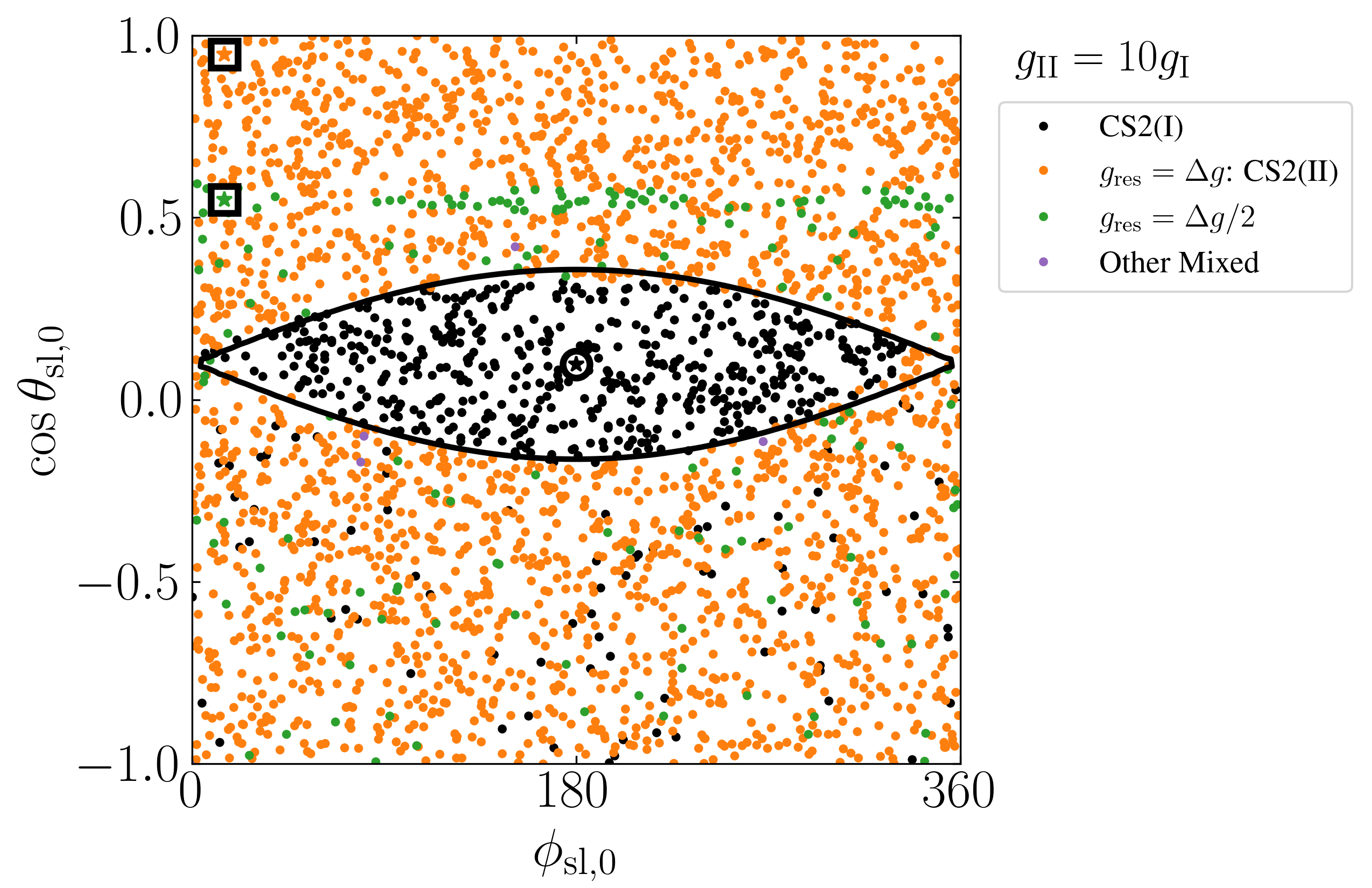
To explore the regimes under which various resonances are important, we numerically determine [by integrating Eqs. (2), (6), and (7)] the final spin equilibria (steady states) for systems with different mode parameters ($I_{\rm(I)}$, $I_{\rm(II)}$, $g_{\rm(I)}$, and $g_{\rm(II)}$), starting from all possible initial spin orientations. Fig. 3 shows some examples of such a calculation for $I_{\rm(I)}=10^{\circ}$, $I_{\rm(II)}=1^{\circ}$, $g_{\rm(I)}=-0.1\alpha$ (the same as in Figs. 1–2), but with the four different values of $g_{\rm(II)}=\left\{0.1,2.5,3.5,10\right\}\times g_{\rm(I)}$. We identify three qualitatively different regimes:

• •

  When $\left|g_{\rm(II)}\right|\ll\left|g_{\rm(I)}\right|$ (top-left panel of Fig. 3), mode II serves as a slow, small-amplitude perturbation to the dominant mode I, and the spin evolution is very similar to that studied in Su & Lai (2021): prograde initial conditions (ICs) outside of the mode-I resonance evolve towards CS2(I), ICs inside the resonance evolve to CS2(I), and retrograde ICs outside of the mode-I resonance reach one of the two probabilistically.

• •

  When $\left|g_{\rm(II)}\right|\sim\left|g_{\rm(I)}\right|$ (see the top-right and bottom-left panels of Fig. 3), the resonances corresponding to the two modes overlap, chaotic obliquity evolution occurs (see Touma & Wisdom, 1993; Laskar & Robutel, 1993), and we expect that CS2(I) becomes less stable²²2An more precise resonance overlap condition can be obtained by comparing the separatrix widths, as the mode-II resonance is much narrower even when $g_{\rm(I)}=g_{\rm(II)}$. Such a condition would require $g_{\rm(I)}\sin I_{\rm(I)}\sim g_{\rm(II)}\sin I_{\rm(II)}$. Thus, the onset of chaos due to resonance overlap occurs somewhere in the range $I_{\rm(II)}/I_{\rm(I)}\lesssim g_{\rm(II)}/g_{\rm(I)}\lesssim 1$.. Indeed we see that in this regime, fewer ICs evolve into the high-obliquity CS2(I) equilibrium of the dominant mode I, and most ICs lead to the low-obliquity CS1(I).

• •

  When $\left|g_{\rm(II)}\right|\gg\left|g_{\rm(I)}\right|$ (see the bottom-right panel of Fig. 3), the separatrix for mode II does not exist, we see that all ICs inside the separatrix of mode I again converge successfully to CS2(I), and CS2(II) becomes the preferred low-obliquity equilibrium. Additionally, a narrow band of ICs with $\cos\theta_{\rm sl,0}\sim 0.6$ and some other scattered ICs with $\cos\theta_{\rm sl,0}\lesssim 0.6$ evolve to the mixed-mode equilibrium with $g_{\rm res}=\Delta g/2$, which has $\theta_{\rm eq}\approx 60^{\circ}$. A second mixed-mode resonance with $g_{\rm res}=\Delta g/3$ is also observed (with $\theta_{\rm eq}\approx 67^{\circ}$) for a sparse set of ICs.

Towards a better understanding of how systems are captured into these mixed-mode equilibria, we numerically calculate the “basin of attraction” by repeating the procedure for producing Fig. 3 but instead use a fine grid of ICs with $\theta_{\rm sl,0}$ near the average obliquity of the equilibrium. This results in a “zoomed-in” version of the bottom-right panel of in Fig. 3 and doubles as a numerical stability analysis of the equilibrium. Figure 4 shows the result of this procedure applied to the $g_{\rm res}=\Delta g/2$ resonance, where we have zoomed in to $\theta_{\rm sl,0}$ near the $\theta_{\rm eq}\approx 60^{\circ}$ associated with the resonance. We see that the resonance is reached consistently from some well-defined regions in the $\left(\theta_{\rm sl},\phi_{\rm sl}\right)$ space.

Figure 5 summarizes the equilibrium obliquities $\theta_{\rm eq}$ of various resonances achieved for the system depicted in the bottom-right panel of Fig. 3. For a trajectory that reaches a particular equilibrium, we compute $\theta_{\rm eq}=\left\langle\theta_{\rm sl}\right\rangle$ by averaging over the last $100/\max\left(\left|g_{\rm(I)}\right|,\left|\Delta g\right|\right)$ of the integration. We obtain the corresponding “resonance” frequency by $g_{\rm res}\simeq\left\langle\dot{\phi}_{\rm sl}\right\rangle$.

In fact, the relation between $\theta_{\rm eq}$ and $g_{\rm res}$ can be described analytically. We consider the equation of motion in the rotating frame where $\hat{\boldsymbol{\mathbf{L}}}=\hat{\boldsymbol{\mathbf{z}}}$ is constant and $\hat{\boldsymbol{\mathbf{J}}}$ lies in the $xz$ plane (i.e. $\hat{\boldsymbol{\mathbf{J}}}=-\sin I\hat{\boldsymbol{\mathbf{x}}}+\cos I\hat{\boldsymbol{\mathbf{z}}}$):

Let $\hat{\boldsymbol{\mathbf{S}}}=\sin\theta_{\rm sl}\left(\cos\phi_{\rm sl}\hat{\boldsymbol{\mathbf{x}}}+\sin\phi_{\rm sl}\hat{\boldsymbol{\mathbf{y}}}\right)+\cos\theta_{\rm sl}\hat{\boldsymbol{\mathbf{z}}}$. The evolution of $\phi_{\rm sl}$ then follows

Note that the single-mode CSs satisfy Eq. (11) where $\dot{\Omega}=g$, $\dot{I}=0$, and $\phi_{\rm sl}$ is either equal to $0^{\circ}$ or $180^{\circ}$ (Eq. 8). For the general, two-mode problem, if $\phi_{\rm res}=\phi_{\rm sl}-g_{\rm res}t$ is a resonant angle, then it must satisfy

where the angle brackets denote an average over a libration period. Since $\phi_{\rm sl}$ circulates when $g_{\rm res}\neq 0$, $\left\langle\cos\phi_{\rm sl}\right\rangle=\left\langle\sin\phi_{\rm sl}\right\rangle=0$. Furthermore, if $I_{\rm(II)}/I_{\rm(I)}\equiv\epsilon\ll 1$, we can expand Eq. (5) to obtain

where $\Delta g\equiv g_{\rm(II)}-g_{\rm(I)}$. To leading order, we have $\dot{\Omega}\simeq g_{\rm(I)}$ and $I\simeq I_{\rm(I)}$, so Eq. (11) reduces to

This is Eq. (15) in the main text, and is shown in Fig. 5. Good agreement between the analytic expression and numerical results is observed. Note that setting $g_{\rm res}=\Delta g$ in Eq. (15) does not yield the mode II CSs, as the mode I inclination is still being used, and the $\phi_{\rm sl}$ terms are averaged out in the mixed mode calculation while being nonzero in the CS obliquity calculation.

The four systems shown in Fig. 3 demonstrate that the characteristic spin evolution depends strongly on the ratio $g_{\rm(II)}/g_{\rm(I)}$. To understand the transition between these different regimes, we vary $g_{\rm(II)}$ over a wide range of values (while keeping the other parameters the same as in Fig. 3). For each $g_{\rm(II)}$, we numerically determine the steady-state (equilibrium) obliquities and compute the probability of reaching each equilibrium by evolving $3000$ initial spin orientations drawn randomly from an isotropic distribution. Figure 6 shows the result. Two trends can be seen: the probability of long-lived capture into the CS2(I) resonance decreases as $\left|g_{\rm(II)}\right|$ is increased from $\left|g_{\rm(II)}\right|\ll\left|g_{\rm(I)}\right|$ to $\left|g_{\rm(II)}\right|\sim\left|g_{\rm(I)}\right|$, and mixed-mode resonances become significant, though non-dominant, outcomes for $\left|g_{\rm(II)}\right|\gg\left|g_{\rm(I)}\right|$.

Having discussed how the spin evolution changes when $g_{\rm(II)}$ is varied, we now explore the effect of different values of $I_{\rm(II)}$. In Fig. 7, we display the final outcomes as a function of the initial spin orientation for the same $g_{\rm(II)}$ values as in Fig. 3, but for $I_{\rm(II)}=3^{\circ}$. Comparing the bottom-left panels of Figs. 3 and 7 (with $g_{\rm(II)}=3.5g_{\rm(I)}$), we find that the favored low-obliquity CS changes from CS1(I) to CS1(II) when using $I_{\rm(II)}=3^{\circ}$. In both cases, CS2(I) is destabilized such that most initial conditions converge to the low-obliquity CS, either CS1(I) or CS1(II). In the bottom-right panel, we find that many initial conditions converge to other mixed modes than the $g_{\rm res}=\Delta g/2$ mode. The values of $g_{\rm res}$ observed for the system are shown in Fig. 8, where we find that many low-order rational multiples of $g_{\rm res}/\Delta g$ are obtained. While the amplitude of oscillation in the final $\theta_{\rm sl}$ is substantial (and larger than in Fig. 5), we find that the predictions of Eq. (15) are consistent up to the range of oscillation of $\theta_{\rm sl}$. In Fig. 9, we summarize the outcomes of spin evolution as a function of $g_{\rm(II)}/g_{\rm(I)}$ for $I_{\rm(II)}=3^{\circ}$. We identify the same two qualitative trends as seen in Fig. 6: the instability of CS2(I) when $g_{\rm(II)}\sim g_{\rm(I)}$ and the appearance of mixed modes when $\left|g_{\rm(II)}\right|\gg\left|g_{\rm(I)}\right|$.

We now briefly discuss the spin evolution of the system incorporating the full tidal effects. In the weak friction theory of the equilibrium tide, the spin orientation and frequency jointly evolve following (Alexander, 1973; Hut, 1981; Lai, 2012)

where

(see Eq. 1, but with $4k=1$).

Since $\alpha\propto\Omega_{\rm s}$ evolves in time, we describe the spin-orbit coupling by the parameter

To facilitate comparison with the previous results, we use $\alpha_{\rm sync}=10\left|g_{\rm(I)}\right|$ and $\left|g_{\rm(I)}\right|t_{\rm s}=300$. Note that for the physical parameters used in Eqs. (4) and (18), $g_{\rm(I)}t_{\rm s}\sim 10^{4}$; we choose a faster tidal timescale to accelerate our numerical integrations. The initial spin is fixed $\Omega_{\rm s,0}=3n$. We then integrate Eqs. (2), (6), and (16–17) starting from various initial spin orientations and determine the final outcomes. Figure 10 shows the results for a few select values of $g_{\rm(II)}$ and for $I_{\rm(II)}=3^{\circ}$. Similar behaviors to Figs. 3 and 7 are observed. The probabilities and obliquities of the various equilibria are shown in Fig. 11. Note that each equilibrium obliquity has a corresponding equilibrium rotation rate, given by

The probabilities shown in Fig. 11 exhibit qualitative trends that are quite similar to those seen for the evolution driven by the tidal alignment torque alone: when $\left|g_{\rm(II)}\right|\ll\left|g_{\rm(I)}\right|$, the results of (Su & Lai, 2021) are recovered; when $g_{\rm(II)}\sim g_{\rm(I)}$, the probability of attaining CS2(I) is significantly suppressed; and when $\left|g_{\rm(II)}\right|\gg\left|g_{\rm(I)}\right|$, mixed modes appear.

In this work, we have shown that the planetary spins in compact systems of multiple super-Earths (SEs), possibly with an outer cold Jupiter companion, can be trapped into a number of spin-orbit resonances when evolving under tidal dissipation, either via a tidal alignment torque (Section 3) or via weak tidal friction (Section 4). In addition to the well-understood tidally-stable Cassini States associated with each of the orbital precession modes, we have also discovered a new class of “mixed mode” spin-orbit resonances that yield substantial obliquities. These additional resonances constitute a significant fraction of the final states of tidal evolution if the planet’s initial spin orientation is broadly distributed, a likely outcome for planets that have experienced an early phase of collisions or giant impacts. For instance, for the fiducial system parameters shown in Fig. 6, these mixed-mode equilibria increase the probability that a planet retains a substantial ($\gtrsim 45^{\circ}$) obliquity from $20\%$ to $30\%$. A large equilibrium obliquity has a significant influence on the planet’s insolation and climate. For planetary systems surrounding cooler stars (M dwarfs), the SEs (or Earth-mass planets) studied in this work lie in the habitable zone (e.g. Dressing et al., 2017; Gillon et al., 2017), and the nontrivial obliquity can impact the habitability of such planets.

In a broader sense, the mixed-mode equilibria discovered in our study represent a novel astrophysical example of subharmonic responses in parametrically driven nonlinear oscillators. In equilibrium, the planetary obliquity oscillates with a period that is an integer multiple of the driving period $2\pi/\left|\Delta g\right|$ (see Appendix A.2 for further discussion). Such subharmonic responses are often seen in nonlinear oscillators (e.g. in the classic van der Pol and Duffing equations Levenson, 1949; Flaherty & Hoppensteadt, 1978; Hayashi, 2014).

Throughout this paper, we have adopted fiducial parameters where $\left|g_{\rm(I)}\right|\lesssim\alpha$, which is generally expected for the SE systems being studied. If instead $\left|g_{\rm(I)}\right|\gtrsim\alpha$, then there is no resonance for the dominant (larger-amplitude) mode I. There are then a few possible cases: if $\left|g_{\rm(II)}\right|\lesssim\alpha$, mode II is both slower than mode I and has a smaller amplitude, so it will not affect the mode I dynamics significantly. On the other hand, if $\left|g_{\rm(II)}\right|\gtrsim\alpha$, then mode II also has no resonance, and both CS2(I) and CS2(II) have low obliquities, implying that the system will always settle into a low-obliquity state.

This work has been supported in part by the NSF grant AST-17152 and NASA grant 80NSSC19K0444. YS is supported by the NASA FINESST grant 19-ASTRO19-0041.

The data referenced in this article will be shared upon reasonable request to the corresponding author.

References

- Adams et al. (2019) Adams A. D., Millholland S., Laughlin G. P., 2019, The Astronomical Journal, 158, 108
- Alexander (1973) Alexander M., 1973, Astrophysics and Space Science, 23, 459
- Armstrong et al. (2014) Armstrong J., Barnes R., Domagal-Goldman S., Breiner J., Quinn T., Meadows V., 2014, Astrobiology, 14, 277
- Benz et al. (1989) Benz W., Slattery W., Cameron A., 1989, Meteoritics, 24, 251
- Bryan et al. (2018) Bryan M. L., Benneke B., Knutson H. A., Batygin K., Bowler B. P., 2018, Nature Astronomy, 2, 138
- Bryan et al. (2019) Bryan M. L., Knutson H. A., Lee E. J., Fulton B., Batygin K., Ngo H., Meshkat T., 2019, The Astronomical Journal, 157, 52
- Bryan et al. (2020) Bryan M. L., et al., 2020, The Astronomical Journal, 159, 181
- Bryan et al. (2021) Bryan M. L., Chiang E., Morley C. V., Mace G. N., Bowler B. P., 2021, The Astronomical Journal, 162, 217
- Colombo (1966) Colombo G., 1966, The Astronomical Journal, 71, 891
- Correia et al. (2003) Correia A. C., Laskar J., de Surgy O. N., 2003, Icarus, 163, 1
- Dai et al. (2018) Dai F., Masuda K., Winn J. N., 2018, The Astrophysical Journal Letters, 864, L38
- Dones & Tremaine (1993) Dones L., Tremaine S., 1993, Science, 259, 350
- Dressing et al. (2017) Dressing C. D., et al., 2017, The Astronomical Journal, 154, 207
- Fabrycky et al. (2007) Fabrycky D. C., Johnson E. T., Goodman J., 2007, The Astrophysical Journal, 665, 754
- Fabrycky et al. (2014) Fabrycky D. C., et al., 2014, The Astrophysical Journal, 790, 146
- Ferreira et al. (2014) Ferreira D., Marshall J., O’Gorman P. A., Seager S., 2014, Icarus, 243, 236
- Flaherty & Hoppensteadt (1978) Flaherty J. E., Hoppensteadt F., 1978, Studies in Applied Mathematics, 58, 5
- Gillon et al. (2017) Gillon M., et al., 2017, Nature, 542, 456
- Groten (2004) Groten E., 2004, Journal of Geodesy, 77, 724
- Hamilton & Ward (2004) Hamilton D. P., Ward W. R., 2004, The Astronomical Journal, 128, 2510
- Hayashi (2014) Hayashi C., 2014, Nonlinear oscillations in physical systems. Princeton University Press
- He et al. (2020) He M. Y., Ford E. B., Ragozzine D., Carrera D., 2020, The Astronomical Journal, 160, 276
- He et al. (2021) He M. Y., Ford E. B., Ragozzine D., 2021, The Astronomical Journal, 161, 16
- Henrard & Murigande (1987) Henrard J., Murigande C., 1987, Celestial Mechanics, 40, 345
- Hong et al. (2021) Hong Y.-C., Lai D., Lunine J. I., Nicholson P. D., 2021, The Astrophysical Journal, 920, 151
- Howard et al. (2012) Howard A. W., et al., 2012, The Astrophysical Journal Supplement Series, 201, 15
- Hut (1981) Hut P., 1981, Astronomy and Astrophysics, 99, 126
- Inamdar & Schlichting (2016) Inamdar N. K., Schlichting H. E., 2016, The Astrophysical Journal Letters, 817, L13
- Izidoro et al. (2017) Izidoro A., Ogihara M., Raymond S. N., Morbidelli A., Pierens A., Bitsch B., Cossou C., Hersant F., 2017, Monthly Notices of the Royal Astronomical Society, 470, 1750
- Jennings & Chiang (2021) Jennings R. M., Chiang E., 2021, Monthly Notices of the Royal Astronomical Society, 507, 5187
- Korycansky et al. (1990) Korycansky D., Bodenheimer P., Cassen P., Pollack J., 1990, Icarus, 84, 528
- Lai (2012) Lai D., 2012, Monthly Notices of the Royal Astronomical Society, 423, 486
- Lainey (2016) Lainey V., 2016, Celestial Mechanics and Dynamical Astronomy, 126, 145
- Laskar & Robutel (1993) Laskar J., Robutel P., 1993, Nature, 361, 608
- Levenson (1949) Levenson M. E., 1949, Journal of Applied Physics, 20, 1045
- Levrard et al. (2007) Levrard B., Correia A. C. M., Chabrier G., Baraffe I., Selsis F., Laskar J., 2007, Astronomy & Astrophysics, 462, L5
- Li (2021) Li G., 2021, The Astrophysical Journal Letters, 915, L2
- Li & Lai (2020) Li J., Lai D., 2020, The Astrophysical Journal Letters, 898, L20
- Li et al. (2021) Li J., Lai D., Anderson K. R., Pu B., 2021, Monthly Notices of the Royal Astronomical Society, 501, 1621
- Lissauer et al. (2011) Lissauer J. J., et al., 2011, The Astrophysical Journal Supplement Series, 197, 8
- Liu et al. (2015) Liu S.-F., Hori Y., Lin D., Asphaug E., 2015, The Astrophysical Journal, 812, 164
- Lobo & Bordoni (2020) Lobo A. H., Bordoni S., 2020, Icarus, 340, 113592
- Masuda et al. (2020) Masuda K., Winn J. N., Kawahara H., 2020, The Astronomical Journal, 159, 38
- Millholland & Batygin (2019) Millholland S., Batygin K., 2019, The Astrophysical Journal, 876, 119
- Millholland & Laughlin (2018) Millholland S., Laughlin G., 2018, The Astrophysical Journal Letters, 869, L15
- Millholland & Laughlin (2019) Millholland S., Laughlin G., 2019, Nature Astronomy, 3, 424
- Millholland & Spalding (2020) Millholland S. C., Spalding C., 2020, The Astrophysical Journal, 905, 71
- Morbidelli et al. (2012) Morbidelli A., Tsiganis K., Batygin K., Crida A., Gomes R., 2012, Icarus, 219, 737
- Murray & Dermott (1999) Murray C. D., Dermott S. F., 1999, Solar system dynamics. Cambridge university press
- Ohno & Zhang (2019) Ohno K., Zhang X., 2019, The Astrophysical Journal, 874, 2
- Peale (1969) Peale S. J., 1969, The Astronomical Journal, 74, 483
- Peale (1974) Peale S. J., 1974, The Astronomical Journal, 79, 722
- Peale (2008) Peale S., 2008, in Extreme Solar Systems. p. 281
- Pu & Lai (2018) Pu B., Lai D., 2018, Monthly Notices of the Royal Astronomical Society, 478, 197
- Rogoszinski & Hamilton (2020) Rogoszinski Z., Hamilton D. P., 2020, The Astrophysical Journal, 888, 60
- Safronov & Zvjagina (1969) Safronov V., Zvjagina E., 1969, Icarus, 10, 109
- Saillenfest et al. (2020) Saillenfest M., Lari G., Courtot A., 2020, Astronomy & Astrophysics, 640, A11
- Saillenfest et al. (2021) Saillenfest M., Lari G., Boué G., 2021, Nature Astronomy, 5, 345
- Sandford et al. (2019) Sandford E., Kipping D., Collins M., 2019, Monthly Notices of the Royal Astronomical Society, 489, 3162
- Seager & Hui (2002) Seager S., Hui L., 2002, The Astrophysical Journal, 574, 1004
- Snellen et al. (2014) Snellen I. A., Brandl B. R., de Kok R. J., Brogi M., Birkby J., Schwarz H., 2014, Nature, 509, 63
- Spiegel et al. (2010) Spiegel D. S., Raymond S. N., Dressing C. D., Scharf C. A., Mitchell J. L., 2010, The Astrophysical Journal, 721, 1308
- Su & Lai (2020) Su Y., Lai D., 2020, The Astrophysical Journal, 903, 7
- Su & Lai (2021) Su Y., Lai D., 2021, Monthly Notices of the Royal Astronomical Society, 509, 3301
- Touma & Wisdom (1993) Touma J., Wisdom J., 1993, Science, 259, 1294
- Tremaine (1991) Tremaine S., 1991, Icarus, 89, 85
- Tremaine & Dong (2012) Tremaine S., Dong S., 2012, The Astronomical Journal, 143, 94
- Vokrouhlickỳ & Nesvornỳ (2015) Vokrouhlickỳ D., Nesvornỳ D., 2015, The Astrophysical Journal, 806, 143
- Ward (1975) Ward W. R., 1975, The Astronomical Journal, 80, 64
- Ward & Canup (2006) Ward W. R., Canup R. M., 2006, The Astrophysical Journal Letters, 640, L91
- Ward & Hamilton (2004) Ward W. R., Hamilton D. P., 2004, The Astronomical Journal, 128, 2501
- Yang et al. (2020) Yang J.-Y., Xie J.-W., Zhou J.-L., 2020, The Astronomical Journal, 159, 164
- Zhu & Wu (2018) Zhu W., Wu Y., 2018, The Astronomical Journal, 156, 92
- Zhu et al. (2018) Zhu W., Petrovich C., Wu Y., Dong S., Xie J., 2018, The Astrophysical Journal, 860, 101
Appendix A Materials and Methods
A.1 Inclination Modes of 3-Planet Systems
In the linear regime, the evolution of the orbital inclinations in a multi-planet system is described by the Laplace-Lagrange theory (Murray & Dermott, 1999; Pu & Lai, 2018). In this section, we consider 3-planet systems. We denote the magnitude of the angular momentum of each planet by and the inclination relative to the total angular momentum axis by , and we define the complex inclination . The evolution equations for , , and are