Dynamically induced conformation depending on excited normal modes of fast oscillation
Abstract
We present dynamical effects on conformation in a simple bead-spring model consisting of three beads connected by two stiff springs. The conformation defined by the bending angle between the two springs is determined not only by a given potential energy function depending on the bending angle, but also fast motion of the springs which constructs the effective potential. A conformation corresponding with a local minimum of the effective potential is hence called the dynamically induced conformation. We develop a theory to derive the effective potential by using multiple-scale analysis and the averaging method. A remarkable consequence is that the effective potential depends on the excited normal modes of the springs and amount of the spring energy. Efficiency of the obtained effective potential is numerically verified.
I Introduction
Conformation is deeply connected with function. A typical example is a biomolecule whose conformation is crucial for binding a ligand koshland-58 ; monod-wyman-changeux-65 ; okazaki-takada-08 ; seeliger-degroot-10 ; fuchigami-etal-11 . Morphological computation hauser-etal-11 ; special-issue-13 ; muller-hoffmann-17 is another example, which can be found for instance as walking robots collins-ruina-tedrake-wisse-05 ; hermans-schrauwen-bienstman-dambre-14 . Mechanical metamaterial mechanical-metamaterials-19 provides several examples like the Miura fold which exhibits negative Poisson’s ratio wei-etal-13 .
Realization of conformations is usually associated with the minimum of a potential energy function. In addition to the potential function, dynamics sometimes contributes to construct an effective potential. A well-known example is the Kapitza pendulum stephenson-08 ; kapitza-51 : An inverted pendulum persists against the gravity by applying a rapidly oscillating external force, since the effective potential provides a local minimum at the inverted position.
We present another dynamical effect on conformation realized in autonomous Hamiltonian systems containing fast and slow motion. Consider a bead-spring model rouse-53 consisting of three beads connected by two stiff springs. The conformation of this system can be identified with the bending angle between the two springs. If the system has a bending potential which depends only on the bending angle, one may imagine that the bending angle goes to a local minimum of the bending potential. The conformation of this system is, however, determined by the effective potential which consists of the bending potential and contribution from the fast spring motion.
More precise description of the above phenomenon is as follows. First of all, the dynamical effect is comparable with the bending potential under the condition that large bending motion is sufficiently slow than the spring motion. The bending potential dominates the effective potential when the spring energy is sufficiently small. However, the dynamical effect enlarges as the spring energy increases, and a local minimum of the effective potential does not necessarily coincide with a local minimum of the bending potential. We call a conformation corresponding to a local minimum of the effective potential a dynamically induced conformation (DIC). Further interesting fact is that the effective potential depends on the excited normal modes of the springs in addition to the spring energy. The three-body bead-spring model has the two normal modes of the springs and each mode makes a different valley.
The three-body system is quite simple, and hence it is theoretically tractable and clearly shows DIC. The aim of this paper is to present the dynamical contribution to conformation in the three-body system. It is worth noting that the bead-spring model mimics several systems: a polymer rouse-53 ; zimm-56 , a microscopic artificial swimmer gauger-stark-06 , a soft magnetic nanowire mirzae-etal-20 , and a semi-flexible macromolecule saadat-khomami-16 .
A theoretical analysis reveals that the essence of DIC is existence of multiple timescales, which is realized in the bead-spring model by stiff springs and slow bending motion. Appearance of multiple timescales is generic in nature. For instance, biomolecules have several forces of diverse strength as strong covalent bonds, intermediate hydrogen bonds, and weak van der Waals forces, and each of them has a characteristic timescale. DIC therefore enriches understanding of the origin of conformation change and its function.
A celebrated example of the dynamically constructed effective potential is found in the aforementioned Kapitza pendulum, and it has been studied in a wide range of fields bukov-dalessio-polkovnikov-15 ; grifoni-hanggi-96 ; wickenbrock-etal-12 ; chizhevsky-smeu-giacomelli-03 ; chizhevsky-14 ; cubero-etal-06 ; bordet-morfu-13 ; weinberg-14 ; uzuntarla-etal-15 ; buchanan-jameson-oedjoe-62 ; baird-63 ; jameson-66 ; apffel-20 ; bellman-mentsman-meerkov-86 ; shapiro-zinn-97 ; borromeo-marchesoni-07 ; richards-etal-18 . The development of the Kapitza pendulum suggests that DIC will provide a large spectrum of applications. Nevertheless, we underline three crucial differences between DIC and the Kapitza pendulum. (i) The bead-spring model is autonomous and the effective potential is intrinsically determined, while one in the Kapitza pendulum can be controlled by the applied external force. (ii) The effective potential depends on the excited normal modes in the bead-spring model. (iii) The local minimum points of the effective potential may continuously move depending on the spring energy in the bead-spring model, while the local minimum created by the external vertical oscillation is fixed at the inverted position in the Kapitza pendulum.
This paper is organized as follows. The three-body bead-spring model is presented in Sec. II with the two important assumptions to have DIC. Following the assumptions, we develop in Sec. III a theory to describe slow bending motion by using a multiple-scale analysis bender-orszag-99 and the averaging method krylov-bogoliubov-34 ; krylov-bogoliubov-47 ; guckenheimer-holmes-83 . The theory provides the effective potential depending on the excited normal modes of the springs and amount of the spring energy. Examples of the effective potential are exhibited in Sec. IV so as to reveal the above dependency. Efficiency of the effective potential is examined through numerical simulations in Sec. V. The final section VI is devoted to summary and discussions.
II Model
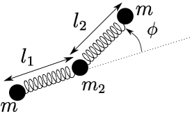
The three-body bead-spring model is sketched in Fig. 1. We assume that the beads move on a two-dimensional plane. The mass and the position of the th bead are respectively denoted by and . The Lagrangian of the model is expressed by
| (1) |
where and is the Euclidean norm: for . The th and the th beads are connected by a stiff spring, and we assume that the two springs have the identical potential. Further, for simplicity, we focus on the symmetric masses: . The term represents the potential energy function, which will be specified later.
We assume that the system described by Eq. (1) has the two-dimensional translational symmetry and the rotational symmetry, which induce the conservation of the two-dimensional total momentum vector and of the total angular momentum, respectively. The total momentum vector can be set as the zero vector without loss of generality, while the total angular momentum is assumed to be zero. The three integrals reduces the system and the reduced Lagrangian is
| (2) |
where
| (3) |
and the superscript T represents transposition. The variables and are the lengths of the two springs,
| (4) |
and is the bending angle,
| (5) |
where is the Euclidean inner product. The function is the element of the size- symmetric matrix , whose explicit form is given in Appendix A. The potential energy function consists of the two parts as
| (6) |
We call and the spring potential and the bending potential, respectively.
We introduce the two assumptions to realize DIC in the above model. Let be a dimensionless small parameter as . The two assumptions are:
-
(A1)
The amplitudes of the springs are sufficiently small comparing with the natural length. The ratio is of .
-
(A2)
Large bending motion is sufficiently slow than the spring motion. The ratio of the two timescales is of .
These two assumptions lead the effective potential for the bending angle . A local minimum point of the effective potential does not necessarily coincide with a local minimum point of the bending potential . That is, the bending angle oscillates around an angle at which the bending potential does not take a local minimum. We develop a theory to derive the effective potential in Sec.III.
III Theory
From now on, we use the Einstein notation for the sum: We take the sum over an index if it appears twice in a term. We derive the equation of motion for the slow bending motion, and construct the effective potential induced by the fast spring motion. A review of the Kapitza pendulum is provided in Appendix B, which might be helpful to understand the theory.
III.1 Multiscale analysis and averaging
The Euler-Lagrange equations derived from Eq. (2) are
| (7) |
where . These equations are the starting point of our theory.
The assumption (A2) induces the two timescales of and . The fast timescale describes the fast spring motion, and the slow timescale corresponds to the slow bending motion. The two timescales transform the time derivative into
| (8) |
From the assumptions (A1) and (A2) the variables and are expanded as
| (9) |
where is the natural length of the two springs. As we will observe later, the fast motion of is induced by the fast motion of the springs and is of the same order as the spring amplitudes. We are interested in , which represents large and slow bending motion. We denote the above expansions for simplicity as
| (10) |
We further expand the potential energy function . The spring potential is assumed to be expanded into the Taylor series around the natural length as
| (11) |
That is, the two springs have the same spring constant
| (12) |
The bending potential is assumed to be expanded into the series of as
| (13) |
The two assumptions (A1) and (A2) induce
| (14) |
as shown in Appendix C, and hence the leading term of is of . This ording results from the assumption (A2): The force from the bending potential should be weaker than that of the spring potential .
We construct the equations of motion order by order, by substituting Eqs. (8), (10), (11), and (13) into Eq. (7). In , we have no terms, because , , and .
In we have
| (15) |
The size- matrix is defined by
| (16) |
where
| (17) |
See Appendix D for the explicit form of . The third column vector of is the zero vector, and the right-hand side of Eq. (15) has no contribution from the third element of , namely . The fast motion of is hence induced by and , as mentioned after Eq. (9).
The slow motion of is described in , and the equation of motion for is
| (18) |
Here is the first order part of and . The explicit forms are
| (19) |
Equation (18) contains the fast oscillation of , and we eliminate it by taking the average over the fast timescale . The average is defined by
| (20) |
for an arbitrary function . After taking the average and recalling , Eq. (18) is simplified to
| (21) |
The right-hand side represents the force, and the averaged term
| (22) |
represents the effective force yielded by the fast spring motion. Here Tr represents the matrix trace. The right-hand side of Eq. (22) depends on and . The dependence can be regarded as the dependence, since and is constant. depends on and , and the dependence is averaged out. We have to eliminate the dependence to obtain the effective potential as a function of .
III.2 Explicit form of the averaged term
We compute the explicit form of the averaged term by performing the diagonalization of Eq. (15), and observe the dependence, which has to be eliminated. Let diagonalize as
| (23) |
The diagonal matrix consists of the eigenvalues of and is denoted by
| (24) |
where
| (25) |
and
| (26) |
A diagonalizing matrix is
| (27) |
with
| (28) |
The three column vectors , and are eigenvectors of , and we call the three modes as the in-phase mode, the anti-phase mode, and the zero-eigenvalue mode, respectively.
To solve Eq. (15), we perform the change of variables as
| (29) |
and solves the diagonalized equations
| (30) |
Denoting the amplitudes of the in-phase and the anti-phase modes by and respectively, which evolve in the slow timescale through the coupling with , and setting the amplitude of the zero-eigenvalue mode as zero, we introduce the diagonal matrix
| (31) |
Putting all together and remembering that the average of the square of a sinusoidal function is , we have
| (32) |
The averaged term contains the two evolving amplitudes and . The untrivial evolution of the amplitudes differs from the Kapitza pendulum, which also contains the amplitude of the external oscillation but it is explicitly given. We have to eliminate the two unknown amplitudes from the averaged term to obtain a closed equation for .
III.3 Hypothesis and energy conservation
The strategy to eliminate the two unknown amplitudes and is as follows. First, we introduce a hypothesis, which is inspired from the adiabatic invariant. The hypothesis reduces the number of unknown variables from two to one. Second, we eliminate the remaining unknown variable by using the energy conservation law.
The first step is the introduction of the hypothesis expressed by
| (33) |
where and are constants satisfying
| (34) |
A physical interpretation of the hypothesis (H) is that the slow bending motion exchanges energy with the fast spring motion in proportion to its normal mode energy. Validity of the hypothesis (H) is examined in Appendix E. We note that the hypothesis should be valid if the modification of is sufficiently small. The unique unknown variable is now , while the constants and have been included in the equations of motion.
The second step is the energy conservation. The leading order of the total energy is of and we expand it as . The leading term is
| (35) |
Taking the average over , we have
| (36) |
Substituting Eq. (33), the unique unknown variable is obtained as
| (37) |
where we denoted by for simplicity. Finally, we eliminate the unknown amplitudes from the averaged term represented in Eq. (32) by substituting Eqs. (33) and (37):
| (38) |
where
| (39) |
We underline that the averaged term depends on the constants and .
III.4 Final result
Substituting Eq. (38) into Eq. (21), we have
| (40) |
where
| (41) |
| (42) |
and
| (43) |
Equation (40) is the closed equation for the slow bending motion. It is reproduced as the Euler-Lagrange equation of the effective Lagrangian
| (44) |
Here, the effective (dimensionless) mass is
| (45) |
and the effective potential is
| (46) |
Note that the physical dimension of differs from due to the factor .
IV Effective potential
We exhibit examples of the effective potential with varying the parameters and (remember ). The equal mass condition is assumed unless there is a notice. Note that the in-phase (anti-phase) mode is the mode- (mode-) as defined in Sec. III.2.
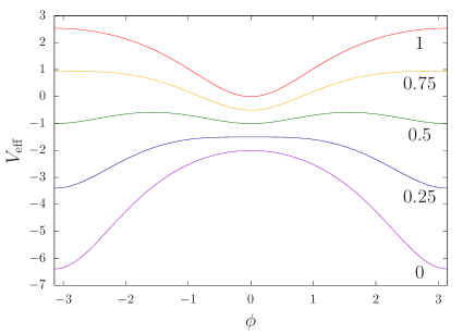
IV.1 Examples without bending potential
First of all, we observe the effective potential without bending potential, , to observe the simplest case. We exhibit effective potentials for some values of () in Fig. 2. The dynamical contribution is completely opposite between the in-phase mode and the anti-phase mode. The in-phase mode makes a valley at , while the anti-phase mode makes a valley at . A precise analysis reveals that there are the two local minima at and in the interval of . The coexistence interval is generalized to
| (47) |
for any value of . See Appendix F for details.
IV.2 Examples with a bending potential
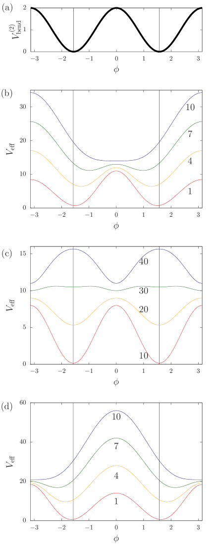
Next, we introduce an example of the bending potential as
| (48) |
This potential has the two minima at . We set the equal mass condition, . Since depends on the normal mode energy distribution and the total energy , we show graphs of the effective potential for (in-phase), (mixed), and (anti-phase) with varying the value of in Fig. 3. The effective potential is similar to the bending potential when the total energy is small. As the total energy increases, the local minimum points move from towards and/or . The local minimum points of are the dynamically induced conformations (DICs).
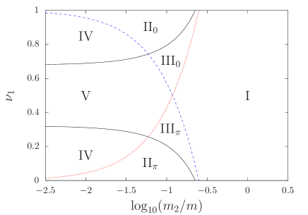
The effective potential is determined at each point on the plane, and yields the set of the local minimum points. We categorize the local minimum points into the three classes: , and . The three classes induce the seven types of sets as arranged in Table 1. By using the seven types, the plane is divided into regions each of which is assigned by a type of the set as reported in Fig. 4. We stress that the seven types are realized by changing the total energy and the mode energy distribution .
| Conformation | I | II0 | IIπ | III0 | IIIπ | IV | V |
|---|---|---|---|---|---|---|---|
| M | O | O | M | M | O | M | |
| O | M | O | M | O | M | M | |
| O | O | M | O | M | M | M |
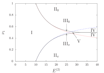
Finally, we present a phase diagram by varying the center mass with fixing in Fig. 5. We give two remarks. First, the seven types are also realized by changing the center mass . The regions assigned by the types III0, IIIπ, IV, and V are enhanced comparing with Fig. 4. This fact suggests that the mass distribution is useful to control the conformation. Second, the dynamical contribution dominates the effective potential when is small. This domination can be explained from Eq. (39), which is a part of the averaged term , and Eq. (26), which is the definitions of and . We have as from Eq. (26). Thus, the denominators of the function can be close to near , and hence contribution from the averaged term becomes large.
V Numerical tests
We verify efficiency of the effective potential through numerical simulations of the model.
V.1 Setting
Numerical simulations are performed by using the fourth order symplectic integrator yoshida-90 for the Hamiltonian
| (49) |
which is the Legendre transform of Eq. (1). The time step is set as . The relative energy error is suppressed in the reported simulations as , where and are respectively the initial energy and the numerically obtained energy.
The two springs are assumed to be linear and is
| (50) |
because the theory includes only the linear part of the springs. The bending potential is , and we use Eq. (48) as . The small parameter is fixed as . The masses are equal and . The spring constant is , and the natural length is .
V.2 Initial condition
We set the initial condition as follows. All the beads have zero initial velocities in the - and -directions. The beads are once placed at the natural lengths of the springs with the bending angle . Then, under the hypothesis (H), we give small displacements of , and so as to excite the normal modes of the springs for a given pair of . The initial condition, denoted by the subscript , is summarized as
| (51) |
See Eq. (27) for the definitions of and . We note that the amplitude is of . In the Hamiltonian system of Eq. (49), a corresponding initial condition is
| (52) |
where is the two-dimensional zero vector. The above initial condition gives the second order total energy as
| (53) |
In the next section we set , which is a local minimum point of the bending potential . The initial condition Eq. (51) hence has two free parameters of the amplitude , which is equivalent with through Eq. (53), and the normal mode energy ratio (remember ).
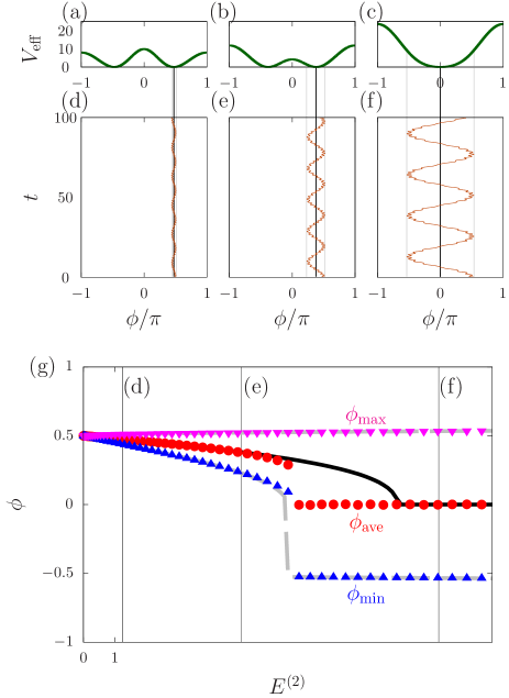
V.3 Efficiency of the effective potential
We concentrate on the in-phase mode, . Temporal evolution of is exhibited in Figs. 6(d), (e), and (f) for three values of , corresponding to three values of [see Eq. (53)]. Small and fast oscillation of comes from and is induced from , which are governed by Eq. (15). When the amplitude is small, the bending angle almost stays around the initial value [Fig. 6(d)], as it is predicted from the bending potential . However, the amplitude of oscillation of becomes large as gets large, and the center of oscillation approaches to the zero [Figs. 6(e) and (f)]. We estimate the center of oscillation by the time average
| (54) |
The estimated center is plotted as a function of in Fig. 6(g) with the minimum and the maximum of in .
Two remarks are in order. First, the minimum and the maximum of are well predicted by . There is a gap between and the bottom of in the energy interval approximated by . The gap is not a counterevidence but a supporting evidence of the theory. This gap comes from the inequality , which implies that the bending angle climbs over the saddle point at . This passing is confirmed by the jump of the theoretical minimum value of . Second, the center of oscillation is continuously modified as the spring energy increases. The conformation is determined not by a local minimum of the bending potential but by a local minimum of the effective potential derived from dynamics. We conclude that the effective potential successfully predicts the slow bending motion.
We provide movies in Supplemental Material SM to show dynamics of the system. See Appendix G for explanation on the movies.
VI Summary and discussions
We have investigated the three-body bead-spring model and demonstrated the dynamically induced conformation (DIC). The fast motion of the springs induces the effective potential for the slow bending motion, and the conformation is governed by the bottoms of the effective potential instead of the bending potential. One crucial remark is that the effective potential depends on the excited normal modes and its energy: The effective potential tends to have the minimum at (), by exciting the in-phase (anti-phase) mode. Moreover, a mixed mode makes the two local minima at and .
We have developed a theory to derive the effective potential based on the multiple-scale analysis and the averaging method. The main idea of the theory is to introduce a hypothesis inspired from the adiabatic invariant. The hypothesis with the energy conservation law eliminate the unknown variables being unavoidable in autonomous systems, and the elimination introduces the mode dependence and the total energy dependence into the effective potential. A theory for a generic system can be found in Refs. yamaguchi-etal-21 ; yamaguchi-22 .
Efficiency of the theoretically obtained effective potential is successfully examined through numerical simulations. The bending angle oscillates in general, and the center of oscillation is not a bottom of the bending potential, but a bottom of the effective potential. An extreme example is that a local maximum point of the bending potential becomes a local minimum point of the effective potential. The amplitude of the bending angle oscillation is also predicted by the effective potential.
The studied model is quite simple as we neglected the excluded volume effect, for instance. The potential of the excluded volume effect, and any other potentials between the two beads of the ends, can be treated in the same way as the bending potential discussed in this article (see Appendix H). Therefore, the phenomenon of DIC is universal as long as the two assumptions (A1) and (A2) hold.
We give three discussions on DIC revealed in this article: universality, application to control, and the beat effect. First, DIC must be universal since the essential mechanism to have DIC is existence of multiple timescales. Indeed, numerical simulations show that -body bead-spring systems exhibit DIC yanagita-konishi-jp . Details will be reported elsewhere. Second, it is interesting to use DIC for controlling the conformation of proteins by changing energy. Control of a robot is also an interesting subject by changing the center mass as shown in Fig. 5. Finally, we have neglected the beat effect between the eigenfrequencies of the fast springs, namely at . The beat effect may trigger the Arnold diffusion arnold-64 since the full dynamics has the three degrees of freedom, (see, for example, Refs. manikandan-keshavamurthy-14 ; firmbach-etal-18 for the recent progress on systems of three degrees of freedom). It will be interesting to observe evolution of the system in a very long time beyond the slow timescale .
Acknowledgements.
Y.Y.Y. acknowledges the support of JSPS KAKENHI Grant Numbers 16K05472 and 21K03402. T.Y. acknowledges the support of JSPS KAKENHI Grant Numbers 18K03471 and 21K03411. T.K. is supported by Chubu University Grant (A). M.T. is supported by the Research Program of ”Dynamic Alliance for Open Innovation Bridging Human, Environment and Materials” in ”Network Joint Research Center for Materials and Devices”, and a Grant-in-Aid for Scientific Research (C) ( No. 22654047, 25610105, and 19K03653 ) from JSPS. The authors express their thanks to the anonymous referees who suggested to input the bending potential.Appendix A Lagrangians of the three-body bead-spring model
The system of Eq. (1) has the two-dimensional translational symmetry and the rotational symmetry. We reduce Eq. (1) and derive Eq. (2) by introducing the internal coordinates. For the reduction we perform three changes of variables.
The first change of variables introduces the vectors along the springs, denoted by and , with the center-of-mass . This change of variables is expressed as
| (55) |
with the total mass
| (56) |
Since each element of is a cyclic coordinate by an assumption and is conserved, we set without loss of generality. This setting reduces and from the Lagrangian, which is written as
| (57) |
where we assumed that the potential energy function depends on only and . is the element of the size- matrix , which is defined by
| (58) |
The second change of variables introduces the polar coordinates , where is the length of and is the angle of measured from a fixed direction on . The vectors and are then written as
| (59) |
where is the unit vector to the radial direction of , and is the unit vector to the angle direction.
As the third change of variables, we define
| (60) |
where represents the bending angle (see Fig. 1). The variables and describes the Lagrangian
| (61) |
where and does not depend on by the assumption of rotational symmetry. The four-dimensional vector is represented by to distinguish from the three-dimensional vector used in Eq. (2). is the element of the size- matrix . The matrix is symmetric, and we show only the upper triangle elements. The diagonal elements are
| (62) |
and the off-diagonal elements are
| (63) |
The Lagrangian of Eq. (61) does not depend on and is a cyclic coordinate. The conjugate momentum , which corresponds to the total angular momentum, is defined by
| (64) |
and is conserved. Eliminating from the kinetic energy, we obtain the Lagrangian
| (65) |
where we identified and since does not depend on . Assuming , we obtain Eq. (2) because contribution from to the Euler-Lagrange equation vanishes. The element of the size- symmetric matrix is defined by
| (66) |
The diagonal elements are
| (67) |
and the off-diagonal elements are
| (68) |
Appendix B Kapitza pendulum
We review an analysis of the Kapitza pendulum. This review is adjusted to our theory for easily capturing a road map of long computations.
We consider a pendulum on the plane where the axis points to the upward direction of the gravity . The pendulum has the length and a point mass at the tip. The angle is taken from the downward direction of the axis to the anti-clockwise direction. An external force oscillates the pivot of the pendulum along the axis with the amplitude and the frequency . The position of the point mass is then written as
| (69) |
where is the initial phase of the pivot. Constructing the Lagrangian, we have the Euler-Lagrange equation for as
| (70) |
where and . If no external oscillation is applied to the pivot, namely , the unique stable stationary point is clearly .
We assume that (i) the amplitude of the oscillating pivot is much smaller than the pendulum length and is of , (ii) the frequency is much smaller than and is of , where is a dimensionless small parameter. These assumptions imply
| (71) |
where and are of .
We introduce two timescales of
| (72) |
which induce
| (73) |
The angle is also expanded as
| (74) |
Substituting the above expansions into the Euler-Lagrange equation, Eq. (70), we have the expanded equation
| (75) |
The equation to is
| (76) |
Solving the above equation with avoiding secular terms, we have
| (77) |
The equation to is
| (78) |
Substituting the solution Eq. (77) and averaging over the fast timescale , we have
| (79) |
The effective potential satisfying
| (80) |
is then obtained as
| (81) |
This effective potential has a local minimum at for in addition to . The inverted pendulum (i.e. ) is therefore stabilized by sufficiently fast oscillation (i.e. small ) of the pivot irrespective of the initial phase .
Appendix C Order of the bending potential
We show and under the assumptions (A1) and (A2).
C.1
There is no time derivative term in , and we have
| (82) |
The zeroth order term is hence constant, and we can set without loss of generality. We note that the identical zero is induced because in Eq. (82) is a variable. The spring potential is not identically zero in general because it is required to hold in
| (83) |
at the point .
C.2
The terms of constructs
| (84) |
where
| (85) |
The first term of the right-hand side in Eq. (85) is zero since , and there is no restoring force for the variable , while Eq. (83) does not imply the zero restoring force for the springs. The second term is constant in the timescale . If the second term is not zero, has a secular term, and the secular term breaks the perturbation expansion Eq. (10), which assumes . Therefore, the second term must be zero and we can set without loss of generality.
Appendix D Matrices in the equations of
We give the explicit forms of the matrix appearing in Eq. (15). The inverse matrix of at is
| (86) |
The matrix is hence
| (87) |
Appendix E Validity of the hypothesis
Under the equal mass condition , we examine validity of the hypothesis (H) expressed in Eq. (33). We introduce the approximations of
| (88) |
and the amplitudes of normal modes are expressed as
| (89) |
where the eigenvalues and are defined in Eq. (25). We compute the normal mode energy ratio defined by
| (90) |
The hypothesis is valid if is constant in time.
We use the initial condition of Eq. (51) with , and the amplitude of the normal modes is . Temporal evolution of is exhibited in Fig. 7 for , and with . The hypothesis (H) is valid around and in particular.
Appendix F Analysis of the effective potential
Let us study the critical points of the effective potential . A critical point is defined as the point at which . The derivative of is
| (91) |
Thus, we have
| (92) |
since the effective mass is always positive as found in Eq. (45). The effective potential at a critical point takes a local minimum or a local maximum depending on the sign of the second derivative. At a critical point, we have and the second derivative of is
| (93) |
Again from , the sign of is determined by the sign of . Keeping in mind the above discussions, we study the critical points of the effective potential for absence and appearance of the bending potential.
F.1 Absence of the bending potential
The function is proportional to for , and the sinusoidal function in gives the two critical points of and . In addition, there are the other two possible critical points which solve the equation
| (94) |
with and exist in the interval
| (95) |
The derivatives of at and are respectively
| (96) |
and
| (97) |
where we used the relation . The point is hence a local minimum point () if and only if
| (98) |
and the point is a local minimum point () if and only if
| (99) |
The two points and are the local minimum points in the interval of Eq. (95). The periodicity of the effective potential requires the same numbers of local minimum points () and local maximum points (), and hence the critical points are the local maximum points.
F.2 Appearance of the bending potential
We write the function as
| (100) |
where
| (101) |
The effective potential has the critical points at , and satisfying . We separately discuss the second derivative
| (102) |
at a critical point.
F.2.1 The critical points and
The second term of the right-hand side of Eq. (102) is zero, and
| (103) |
This factor is positive (negative) at (), and the sign of is determined by . We have
| (104) |
and
| (105) |
We separately discuss for and , where the boundary comes from the bending potential at and : .
If , the maximum value of is realized at , which gives
| (106) |
for . Note . The point is hence a local maximum point for . A similar discussion states that the point is a local maximum point for .
For , the effective potential takes a local minimum at if
| (107) |
and takes a local minimum at if
| (108) |
By changing the inequalities into the equality, Eq. (107) gives the red dotted-line and Eq. (108) gives the blue dashed-line in Figs. 4 and 5. We remark that Eq. (108) is equivalent with
| (109) |
whose right-hand side is identical with that of Eq. (107).
F.2.2 The critical point
We have , and
| (110) |
The effective potential takes a local minimum (maximum) if () at the critical point .
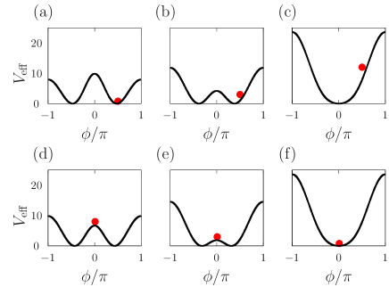
Appendix G Explanation on movies
We provide movies for the initial conformations shown in Fig. 8 in Supplemental Material SM . The bending potential of Eq. (48) is in use. The excited spring mode is , and the amplitude is for Figs. 8 (a) and (d), for (b) and (e), and for (c) and (f). The other initial conditions are described in Sec. V.2, and the system parameter values (, and ) are given in Sec. V.1. Dynamics of the system corresponding to the panels from Figs. 8(a) to (f) is demonstrated in from MovieA to MovieF, respectively. We stress that temporal evolution is well understood by the effective potential , while the bending potential [see Fig. 3(a)] does not explain it.
Appendix H From a general potential to the bending potential
The bending potential represents the interaction between the two beads of the ends, because the interction between an end and the center beads results in the spring potential. We show that the bending potential energy function of is derived from any potential which is a function of the distance , although it is assumed to be a function of only in the main text. Here is represented by using , and as
| (111) |
Substituting Eq. (9) into Eq. (111), we have and
| (112) |
As shown in Appendix C, the potential is of under the assumptions (A1) and (A2), and we expand it as
| (113) |
Therefore, the second order bending potential is derived as a function of only as
| (114) |
The effective potential is obtained from Eq. (46) by substituting the above bending potential into Eq. (42).
References
- (1) D. Koshland, Application of a theory of enzyme specificity to protein synthesis, Proc. Natl. Acad. Sci. USA 44, 98 (1958).
- (2) J. Monod, J. Wyman, and J. P. Changeux, On the nature of allosteric transitions: A plausible model, J. Mol. Biol. 12, 88 (1965).
- (3) K. Okazaki and S. Takada, Dynamic energy landscape view of coupled binding and protein conformational change: Induced-fit versus population-shift mechanisms, PNAS 105, 11182 (2008).
- (4) D. Seeliger and B. L. de Groot, Conformational transitions upon ligand binding: Holo structure prediction from apo conformations, PLoS Comput. Biol. 6, e1000634 (2010).
- (5) S. Fuchigami, H. Fujisaki, Y. Matsunaga, and A. Kidera, Protein functional motions: Basic concepts and computational methodologies, in Advancing theory for kinetics and dynamics of complex, many-dimensional systems: Clusters and Proteins: Advances in Chemical Physics, Volume 145 (Wiley, New Jersey, 2011).
- (6) H. Hauser, A. J. Ijspeert, R. M. Füchslin, R. Pfeifer, and W. Maass, Towards a theoretical foundation for morphological computation with compliant bodies, Biol. Cybern. 105, 355 (2011).
- (7) Special issue on Morphological Computation, Artificial Life 19(1) (2013).
- (8) V. C. Müller and M. Hoffmann, What Is Morphological Computation? On How the Body Contributes to Cognition and Control, Artificial Life 23, 1 (2017).
- (9) S. Collins, A. Ruina, R. Tedrake, and M. Wisse, Efficient bipedal robots based on passive-dynamic walkers, Science 307, 1082 (2005).
- (10) M. Hermans, B. Schrauwen, P. Bienstman, and J. Dambre, Automated design of complex dynamic systems, PLoS ONE 9, e86696 (2014). doi:10.1371/journal.pone.0086696
- (11) J. U. Surjadi, L. Gao, H. Du, X. Li, X. Xiong, N. X. Fang, and Y. Lu, Mechanical metamaterials and their engineering applications, Adv. Eng. Mater. 21, 1800864 (2019).
- (12) Z. Y. Wei, Z. V. Guo, L. Dudte, H. Y. Liang, and L. Mahadevan, Geometric mechanics of periodic pleated origami, Phys. Rev. Lett. 110, 215501 (2013).
- (13) A. Stephenson, XX. On induced stability, The London, Edinburgh, and Dublin Philosophical Magazine and Journal of Science 15, 233 (1908).
- (14) P. L. Kapitza, Dynamic stability of a pendulum when its point of suspension vibrates, Soviet Phys. JETP 21, 588 (1951); Collected papers of P. L. Kapitza, Vol.2, pp.714–737 (1965).
- (15) P. E. Rouse, A theory of the linear viscoelastic properties of dilute solutions of coiling polymers, J. Chem. Phys. 21, 1272 (1953).
- (16) B. H. Zimm, Dynamics of polymer molecules in dilute solution: Viscoelasticity, flow birefringence and dielectric loss, J. Chem. Phys. 24, 269 (1956).
- (17) E. Gauger and H. Stark, Numerical study of a microscopic artificial swimmer, Phys. Rev. E 74, 021907 (2006).
- (18) Y. Mirzae, B. Y. Rubinstein, K. I. Morozov, and A. M. Leshansky, Modeling propulsion of soft magnetic nanowires, Front. Robot. AI 7, 595777 (2020).
- (19) A. Saadat and B. Khomami, A new bead-spring model for simulation of semi-flexible macromolecules, J. Chem. Phys. 145, 024902 (2016).
- (20) M. Bukov, L. D’Alessio, and A. Polkovnikov, Universal high-frequency behavior of periodically driven systems: from dynamical stabilization to Floquet engineering, Advances in Physics 64, 139 (2015).
- (21) M. Grifoni and P. Hänggi, Coherent and incoherent quantum stochastic resonance, Phys. Rev. Lett. 76, 1611 (1996).
- (22) A. Wickenbrock, P. C. Holz, N. A. Abdul Wahab, P. Phoonthong, D. Cubero, and F. Renzoni, Vibrational mechanics in an optical lattice: Controlling transport via potential renormalization. Phys. Rev. Lett. 108, 020603 (2012).
- (23) V. N. Chizhevsky, E. Smeu, and G. Giacomelli, Experimental evidence of “vibrational resonance” in an optical system, Phys. Rev. Lett. 91, 220602 (2003).
- (24) V. N. Chizhevsky, Experimental evidence of vibrational resonance in a multistable system, Phys. Rev. E 89, 062914 (2014).
- (25) D. Cubero, J. P. Baltanas, and J. Casado-Pascual, High-frequency effects in the Fitzhugh-Nagumo neuron model, Phys. Rev. E 73, 061102 (2006).
- (26) M. Bordet and S. Morfu, Experimental and numerical study of noise effects in a FitzHugh–Nagumo system driven by a biharmonic signal, Chaos, Solitons & Fractals 54, 82 (2013).
- (27) S. H. Weinberg, High frequency stimulation of cardiac myocytes: A theoretical and computational study, Chaos 24, 043104 (2014).
- (28) M. Uzuntarla, E. Yilmaz, A. Wagemakers, and M. Ozer, Vibrational resonance in a heterogeneous scale free network of neurons, Commun. Nonlinear Sci. Numer. Simulat. 22, 367 (2015).
- (29) R. H. Buchanan, G. Jameson, and D. Oedjoe, Cyclic migration of bubbles in vertically vibrating liquid columns, Ind. Eng. Chem. Fund. 1, 82 (1962).
- (30) M. H. I. Baird, Resonant bubbles in a vertically vibrating liquid column, Can. J. Chem. Eng. 41, 52 (1963).
- (31) G. J. Jameson, The motion of a bubble in a vertically oscillating viscous liquid, Chem. Eng. Sci. 21, 35 (1966).
- (32) B. Apffel, F. Novkoski, A. Eddi, and E. Fort, Floating under a levitating liquid, Nature 585, 48 (2020).
- (33) R. E. Bellman, J. Bentsman, and S. M. Meerkov, Vibrational control of nonlinear systems, IEEE Trans. Automat. Contr. 31, 710 (1986).
- (34) B. Shapiro and B. T. Zinn, High-frequency nonlinear vibrational control, IEEE Trans. Automat. Contr. 42, 83 (1997).
- (35) M. Borromeo and F. Marchesoni, Artificial sieves for quasimassless particles, Phys. Rev. Lett. 99, 150605 (2007).
- (36) C. J. Richards, T. J. Smart, P. H. Jones, and D. Cubero, A microscopic Kapitza pendulum, Scientific Reports 8, 13107 (2018).
- (37) C. M. Bender and S. A. Orszag, Advanced Mathematical Methods for Scientists and Engineers I: Asymptotic Methods and Perturbation Theory (Springer, 1999).
- (38) N. M. Krylov and N. N. Bogoliubov, New Methods of Nonlinear Mechanics in their Application to the Investigation of the Operation of Electronic Generators. I (United Scientific and Technical Press, Moscow, 1934).
- (39) N. M. Krylov and N. N. Bogoliubov, Introduction to Nonlinear Mechanics (Princeton University Press, Princeton, 1947).
- (40) J. Guckenheimer and P. Holmes, Nonlinear Oscillations, Dynamical Systems, and Bifurcations of Vectgor Fields (Springer-Verlag, New York, 1983).
- (41) T. Yanagita and T. Konishi, Numerical analysis of new oscillatory mode of bead-spring model, Journal of JSCE A2 75, I_125 (2019) (in Japanese).
- (42) H. Yoshida, Construction of higher order symlectic integrators, Phys. Lett. A 190, 262 (1990).
- (43) See Supplemental Material at [URL] for movies.
- (44) Y. Y. Yamaguchi, T. Yanagita, T. Konishi, and M. Toda, Dynamically induced conformation depending on excited normal modes of fast oscillation, arXiv:2111.10025v1.
- (45) Y. Y. Yamaguchi, in preparation.
- (46) V. I. Arnold, Instability of dynamical systems with several degrees of freedom, Sov. Math.-Dokl. 5, 58 (1964).
- (47) P. Manikandan and S. Keshavamurthy, Dynamical traps lead to the slowing down of intramolecular vibrational energy flow, PNAS 111, 14354 (2014).
- (48) M. Firmbach, S. Lange, R. Ketzmerick, and A. Bäcker, Three-dimensional billiards: Visualization of regular structures and trapping of chaotic trajectories, Phys. Rev. E 98, 022214 (2018).