Dynamically encircling an exceptional point in a real quantum system
Abstract
The exceptional point, known as the non-Hermitian degeneracy, has special topological structure, leading to various counterintuitive phenomena and novel applicationsNP_Ganainy ; NPhoton_Feng ; Science_Miri ; Nat.Mater_Ozdemir , which are refreshing our cognition of quantum physics. One particularly intriguing behavior is the mode switch phenomenon induced by dynamically encircling an exceptional point in the parameter spacePRL_Lefebvre ; PRL_Atabek ; JPA_Uzdin ; JPA_Berry ; PRA_Gilary ; PRA_Thomas ; PRL_Hassan ; PRR_Pick . While these mode switches have been explored in classical systemsNature_Doppler ; Nature_Xu ; Nature_Yoon ; PRX_Zhang , the experimental investigation in the quantum regime remains elusive due to the difficulty of constructing time-dependent non-Hermitian Hamiltonians in a real quantum system. Here we experimentally demonstrate dynamically encircling the exceptional point with a single nitrogen-vacancy center in diamond. The time-dependent non-Hermitian Hamiltonians are realized utilizing a dilation method. Both the asymmetric and symmetric mode switches have been observed. Our work reveals the topological structure of the exceptional point and paves the way to comprehensively explore the exotic properties of non-Hermitian Hamiltonians in the quantum regime.
Quantum systems driven by non-Hermitian Hamiltonians exhibit exotic properties comparing to those governed by Hermitian HamiltoniansNP_Ganainy ; NPhoton_Feng . One of the distinct features is the existence of exceptional point (EP), at which both the eigenvalues and the corresponding eigenvectors coalesceCzech.J.Phys_Berry . Classical systems, such as optics and photonics, have provided fertile grounds to investigate EP-related novel phenomena and applicationsScience_Miri ; Nat.Mater_Ozdemir , such as single mode lasers with gain and lossScience_feng ; Science_Hodaei ; Science_Peng , unidirectional invisibilityPRL_Lin ; Nat.Mater_Feng , EP-enhanced mode splittingPRL_Wiersig ; Nature_Chen ; Nature_Hodael ; PRL_Liu and many othersNature_Regensburger ; PRL_Regensburger ; NatMater_Weimann ; NP_Peng . These fascinating processes were realized at or near an EP, but some other important properties of the EP can only be revealed when it is encircled in the parameter space. When the EP is encircled in a quasistatic manner, the two eigenvalues and the corresponding eigenvectors swap with each otherEur.phys_Heiss ; PRE_Heiss ; PRL_Dembowski ; Nature_Gao ; PRX_Ding . The effects due to dynamically encircling EPs have been investigated in classical systemsNature_Doppler ; Nature_Xu ; Nature_Yoon ; PRX_Zhang . Mode switching will emerge when the start points locate at different parity-time-symmetric (-symmetric) phasesPRL_Lefebvre ; PRL_Atabek ; JPA_Uzdin ; JPA_Berry ; PRA_Gilary ; PRA_Thomas ; PRL_Hassan ; PRR_Pick . These mode switches are expected to play an important role in quantum controlPRR_Pick .
We take the following non-Hermitian Hamiltonian as an example to describe the mode switching phenomenon:
| (1) |
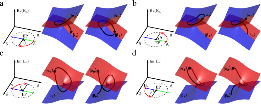
where is a constant number chosen as , and are time-dependent real numbers. Eigenenergies of this Hamiltonian are , and a pair of EPs arises when and . For different and , the real and imaginary parts of are shown in Fig. 1, which displays a complex eigenvalue topology of two intersecting Riemann sheets wrapped around the EP. Dynamically encircling the EP in the parameter space is realized by the time-dependent parameters, and , where is the encircling angle and defines the start point. The encircling direction is decided by the sign of as shown by the red arc with arrow. In Fig. 1a and b, and the start points locate at the -symmetric phase. The encircling initial state is prepared to or which is the eigenstate of the initial Hamiltonian at start point A. When the encircling direction is clockwise, both and will evolve to (Fig. 1a). When the encircling direction is counterclockwise, both and will evolve to (Fig. 1b). The encircling final state depends on the encircling direction, which is taken as the asymmetric mode switching. In Fig. 1c and d, and the start points locate at the -symmetry broken phase. The encircling initial state is prepared to or which is eigenstate of the initial Hamiltonian at start point B. Whether the encircling direction is clockwise (Fig. 1c) or counterclockwise (Fig. 1d), both and will evolve to . This exhibits the symmetric mode switching.
Experimental investigations of phenomena via dynamically encircling EPs have been realized in classical systemsNature_Doppler ; Nature_Xu ; Nature_Yoon ; PRX_Zhang , and the research has remained elusive in the quantum domain. This is because the Hamiltonian of a closed quantum system is Hermitian while the evolution of dynamically encircling an EP is governed by the time-dependent non-Hermitian Hamiltonian. Recently, there have been experiments investigating dynamics of individual quantum systems driven by non-Hermitian HamiltoniansScience_Wu ; NP_M.Naghiloo ; PRB_Partanen . In these works, the Hamiltonians are time-independent, which prevent further investigating important physics driven by time-dependent non-Hermitian Hamiltonians. To overcome this obstacle, we have utilized a dilation method to realize time-dependent non-Hermitian Hamiltonians. Then dynamically encircling an EP has been realized in a single-spin system and mode switches have been observed.
The procedure of dynamically encircling an EP is described by the Schrdinger equation . We introduce an ancilla qubit to construct the dilated state (unnormalized for convenience), where and form an orthogonal basis of the ancilla qubit, and is an appropriate operator given by the dilation method (see Supplementary Note II for details). The evolution of is embedded in the subspace of where the state of the ancilla qubit is . The state is governed by the Hermitian Hamiltonian, , which can be flexibly designed according to practical quantum systems. Here we choose
| (2) |
where , , and is a real function (see Supplementary Note II for details). During the encircling process, the inner product of the encircling state, , covers several orders of magnitude since the evolution under the non-Hermitian Hamiltonian is trace non-conservative. The probability of obtaining the ancilla qubit state , , will be small during some periods of evolution, which makes it difficult to continuously monitor the state evolution of dynamically encircling the EP though selecting the state of the ancilla qubit (see Supplementary Note III for details). To solve this problem, we introduce an alternative measurement method. The dilated state can also be rewritten as . The state of the system qubit is measured when the ancilla qubit state is , which is . Then the state is obtained by multiplying to the state with proper renormalization.
Our scheme is demonstrated in a single nitrogen-vacancy () center in diamond (Fig. 2a). With a static magnetic field applied along the NV symmetry axis, the Hamiltonian of the center can be written as , where GHz is the zero-field splitting of the electron spin, MHz is the nuclear quadrupolar interaction, and MHz is the hyperfine coupling between the electron spin and the nuclear spin. () denotes the Zeeman splitting of the electron (nuclear) spin. and are the spin-1 operators of the electron spin and the nuclear spin, respectively. The subspace spanned by and (black box in Fig. 2b) is encoded as a two-qubit system to construct Hamiltonian . The electron spin is chosen as the system qubit and the nuclear spin is selected as the ancilla qubit. By decomposing and in terms of Pauli operators, we can rewrite the Hamiltonian in Eq.2 as , where , are the decomposition coefficients, and for are Pauli operators. Two selective microwave pulses (red arrows in Fig. 2b) are applied to realize the Hamiltonian . The Hamiltonian of the pulses in the two-qubit system can be written as
| (3) | ||||
The dilated Hamiltonian can be constructed in an interaction picture when the amplitudes, angular frequencies and the phases of the two pulses satisfy the following relations, , , and (see Supplementary Note IV for details).
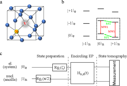
The experiment was implemented on an optically detected magnetic resonance setup. The static magnetic field was set to 500 Gauss in order to polarize the NV center to state by optical pumpingPRL_V.Jacques . When we choose , the initial state of the two-qubit system has the form . The encircling initial state was set to the eigenstate, or ( or ), of the initial Hamiltonian at start point A (B). was prepared by rotation on the nuclear spin followed by rotation on the electron spin (Fig. 2c), where , and depended on the choice of . Then the system evolved under the dilated Hamiltonian by applying two selective pulses given in Eq.3 to realize the dynamically encircling procedure. The total encircling time is set to be . Finally, a state tomography is implemented to measure the state when the ancilla qubit state is . The state is obtained by multiplying the operator on the state with the maximum likelihood estimationPRA_Fiurasek and all the experimental fidelities of and in our experiment are close to 1 (see Supplementary Note III for details).
Fig. 3 displays the results of an asymmetric mode switching when the start point locates at the -symmetric phase. The horizontal axes in Fig. 3 and 4 are rotation angle for clearly demonstration of the encircling process, where with s-1. Fig. 3a and b show the cases of clockwise encircling. In Fig. 3a, we prepared the encircling initial state, , to eigenstate . The overlaps of with and were and , respectively. The non-zero overlap between and is due to the non-orthogonality of the two eigenstates of . Then the encircling state followed the evolution of dynamically encircling the EP characterized by the overlaps with and . After the encircling process, the overlap between the encircling final state and was . This shows that eigenstate will switch to after encircling around the EP, as clarified by the sketch on the diagram. In Fig. 3b, the state was first prepared to and the results show that it returned to after the encircling process. The counterclockwise encircling cases are shown in Fig. 3c and d. The initial states were prepared to and in Fig. 3c and d, respectively. After encircling the EP, the encircling states both evolved to . All the measured evolutions in Fig. 3 show good agreement with the theoretical predictions. These results exhibit that the encircling initial state doesn’t influence the encircling final state. The encircling final state depends on the encircling direction. The evolutions displayed in Fig. 3 unambiguously certifies an asymmetric mode switching when the evolution starts from the -symmetric phase.
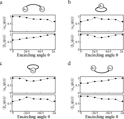
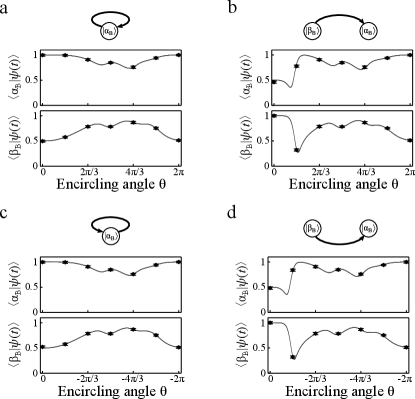
Fig. 4 exhibits the results of a symmetric mode switching when the start point locates at the -symmetry broken phase. The overlaps between the encircling state and the eigenstates, and , were used to describe the evolution. Fig. 4a and b show the cases of clockwise encircling and the initial states were prepared to and , respectively. The counterclockwise encircling cases are presented in Fig. 4c and d. For all these cases, the final states evolved to after the encircling process regardless of the initial state and the path direction. The experimental results agree well with the corresponding theoretical predictions. These results indisputably reveal a symmetric mode switching when initial Hamiltonian is -symmetry broken.
In conclusion, dynamically encircling an EP in a single-spin system has been realized to explore the topological structure of the EP, and both the symmetric and asymmetric mode conversions have been observed. These mode switches provide a robust fashion to control quantum states and thus have great potential in quantum information precessingPRR_Pick . Furthermore, our successful demonstration of engineering time-dependent non-Hermitian Hamiltonians opens a door towards future investigation of complicated dynamical processes governed by time-dependent non-Hermitian Hamiltonians in the quantum realm, such as, encircling high-order EPsJ.Phys.A_Demange ; PRA_Schnabel , researching non-Hermitian geometric phaseJ.Math.Phys_Hossein ; PRA_Gong and studying non-Hermitian topological invariantsJ.Phys_Ananya .
References
- (1) El-Ganainy, R. et al. Non-Hermitian physics and PT symmetry. Nat. Phys. 14, 11-19 (2018).
- (2) Feng, L., El-Ganainy, R. Ge, L. Non-Hermitian photonics based on parity-time symmetry. Nat. Photonics 11, 752-762 (2017).
- (3) Miri, M.-A. Al, A. Exceptional points in optics and photonics. Science 363, eaar7709 (2019).
- (4) zdemir, S. K., Rotter, S., Nori, F. Yang, L. Parity-time symmetry and exceptional points in photonics. Nat. Mater. 18, 783-798 (2019).
- (5) Lefebvre, R., Atabek, O., indelka, M. Moiseyev, N. Resonance coalescence in molecular photodissociation. Phys. Rev. Lett. 103, 123003 (2009).
- (6) Atabek, O. et al. Proposal for a laser control of vibrational cooling in Na2 using resonance coalescence. Phys. Rev. Lett. 106, 173002 (2011).
- (7) Uzdin, R., Mailybaev, A., Moiseyev, N. On the observality of adiabatic state flips generated by exceptional points. J. Phys. A 44, 435302 (2011).
- (8) Berry, M.V., Uzdin, R. Slow non-Hermitian cycling: exact solutions and the Stokes phenomenon. J. Phys. A 44, 435303 (2011).
- (9) Gilary, I., Mailybaev, A. A., Moiseyev, N. Time-asymmetric quantum-state-exchange mechanism. Phys. Rev. A 88, 010102(R) (2013).
- (10) Milburn, T. J. General description of quasiadiabatic dynamical phenomena near exceptional points. Phys. Rev. A 92 052124 (2015).
- (11) Hassan, A. U., Zhen, B., Soljai, M., Khajavikhan, M., Christodoulides, D. N. Dynamically encircling exceptional points: exact evolution and polarization state conversion. Phys. Rev. Lett. 118, 093002 (2017).
- (12) Pick, A., Silberstein, S., Moiseyev, N., Bar.-Gill, N. Robust mode conversion in NV centers using exceptional points. Phys. Rev. Research 1, 013015 (2019).
- (13) Doppler, J. et al. Dynamically encircling an exceptional point for asymmetric mode switching. Nature 537, 76-79 (2016).
- (14) Xu, H., Mason, D., Jiang, L. Harris, J. G. E. Topological energy transfer in an optomechanical system with exceptional points. Nature 548, 80-83 (2016).
- (15) Yoon, J. W. et al. Time-asymmetric loop around an exceptional point over the full optical communication band. Nature 562, 86-90 (2018).
- (16) Zhang, X.-L., Wang, S., Hou, B., Chan, C. T. Dynamically Encircling Exceptional Points: In situ Control of Enclrcling Loops and the Role of the Starting Point. Phys. Rev. X 8, 021066 (2018).
- (17) Berry, M. V. Physics of nonhermitian degeneracies. Czech. J. Phys. 54, 1039-1047 (2004).
- (18) Feng, L., Wong, Z. J., Ma, R.-M., Wang, Y., Zhang, X. Single-mode laser by parity-time symmetry breaking. Science 346, 972-975 (2014).
- (19) Hodaei, H., Miri, M.-A., Heinrich, M., Christodoulides, D. N., Khajavikhan, M. Parity-time-symmetric microring lasers. Science 346, 975-978 (2014).
- (20) Peng, B. et al. Loss-induced supression and revival of lasing. Science 346, 328-322 (2014).
- (21) Lin, Z. et al. Unidirectional invisibility induced by PT-symmetric periodic structures. Phys. Rev. Lett. 106, 213901 (2011).
- (22) Feng, L. et al. Experimental demonstration of a unidirectional reflectionless parity-time metamaterial at optical frequencies. Nat. Mater. 12, 108-113 (2013).
- (23) Wiersig, J. Enhancing the sensitivity offrequency and energy splitting detection by using exceptional points: Application to microcavity sensors for single particle detection. Phys. Rev. Lett. 112, 203901 (2014).
- (24) Chen, W., zdemir, S. K., Zhao, G., Wiersig, J. Yang, L. Exceptional points enhanced sensing in an optical microcavity. Nature 548, 192-196 (2017).
- (25) Hodael, H. et al. Enhanced sensitivity at higher-order exceptional points. Nature 548, 187-191 (2017).
- (26) Liu, Z.-P. et al. Metrology with PT symmetric cavities: Enhanced sensitivity near the PT-phase transition. Phys. Rev. Lett. 112, 203901 (2014).
- (27) Regensburger, A. et al. Parity-time synthetic photonic lattices. Nature 488, 167-171 (2012).
- (28) Regensburger, A. et al. Observation of defect states in -symmetric optical lattices. Phys. Rev. Lett. 110, 223902 (2013).
- (29) Weimann, S. et al. Topologically protected bound states in photonic parity-time-symmetric crystals. Nat. Mater. 16, 433-438 (2017).
- (30) Peng, B. et al. Parity-time-symmetric whispering-gallery microcavities. Nat. Phys. 10, 394-398 (2014).
- (31) Heiss, W. D. Phases of wave functions and level repulsion. Eur. Phys. J. D 7, 1-4 (1999).
- (32) Heiss, W. D. Repulsion of resonance states and exceptional points. Phys. Rev. E 61, 929-932 (2000).
- (33) Dembowski, C. et al. Experimental Observation of the Topological Structure of Exceptional Points Phys. Rev. Lett. 87, 787-790 (2001).
- (34) Gao, T. et al. Observation of non-Hermitian degeneracies in a chaotic exciton-polariton billiard. Nature 526, 554-558 (2015).
- (35) Ding, K., Ma, G., Xiao, M., Zhang, Z. Q., Chan, C. T. Emergence, Coalescence, and Topological Properties of Multiple Exceptional Points and Their Experimental Realization. Phys. Rev. X 6, 021007(2018).
- (36) Wu, Y. et al. Observation of parity-time symmetry breaking in a single spin system. Science 346, 878-880 (2019).
- (37) Naghiloo, M., Abbasi, M., Joglekar, Y.N., Murch, K.W. Quantum state tomography across the exceptional point in a single dissipative qubit. Nat. Phys. 15, 1232-1236 (2019).
- (38) Partanen, M. et al. Exceptional points in tunable superconducting resonators. Phys. Rev. B 100 134505 (2019).
- (39) Jacques, V. et al. Dynamic polarization of single nuclear spins by optical pumping of Nitrogen-Vacancy color centers in diamond at room temperature. Phys. Rev. Lett. 102, 057043 (2009).
- (40) Fiurek, J., Maximum-likelihood estimation of quantum measurement. Phys. Rev. A 64, 024102 (2001).
- (41) Demange, G., Graefe, E.-M. Signatures of three coalescing eigenfunctions. J. Phys. A 45, 025303 (2012).
- (42) Schnabel, J., Cartarius, H., Main, J., Wunner, G., Heiss, W. D. PT-symmetric waveguide system with evidence of a third-order exceptional point. Phys. Rev. A 82, 012103 (2010).
- (43) Mehri.-Dehnavi, H., Mostafazadeh, A. Geometric phase for non-Hermitian Hamiltonians and its holonomy interpretation. J. Math. Phys. 49, 082105 (2008).
- (44) Gong, J., Wang, Q.-h. Geometric Phase in PT-symmetric Quantum Mechanics. Phys. Rev. A 82, 012103 (2010).
- (45) Ghatak, A., Das, T. New topological invariants in non-Hermitian systems. J. Phys. Condens. Matter. 31, 263001 (2019).
.1 Acknowledgements
We thank Qing-Hai Wang for the helpful discussion. This work was supported by the National Key RD Program of China (Grants No. 2018YFA0306600 and No. 2016YFB0501603), the NNSFC (No. 11761131011), the Chinese Academy of Sciences (Grants No. GJJSTD20170001, No.QYZDY-SSW-SLH004 and No.QYZDB-SSW-SLH005), and Anhui Initiative in Quantum Information Technologies (Grant No. AHY050000). X.R. thanks the Youth Innovation Promotion Association of Chinese Academy of Sciences for the support.
.2 Method
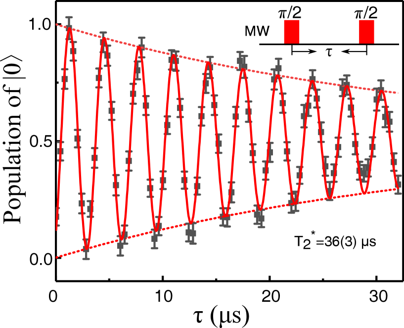
Our experiment was implemented on a NV center in a piece of face bulk diamond which is isotopically purified ([12C]=99.9%). The electron spin qubit was chosen as the system qubit. The dephasing time of the electron spin is (see Supplementary Note I for details).
The sample was placed in a confocal setup. An acousto-optic modulator (ISOMET, AOMO 3200-121) was utilized to modulate the 532 nm green laser pulses. The laser beam traveled twice through the acousto-optic modulator before going through an oil objective (Olympus, PLAPON 60*O, NA 1.42) and then focusing on the NV center. The phonon sideband fluorescence (wavelength, 650-800nm) went through the same oil objective and was collected by an avalanche photodiode (Perkin Elmer, SPCM-AQRH-14) with a counter card. The static magnetic field of 500 G was provided by a permanent magnet along the NV symmetry axis. The state of the two-qubit system can be effectively polarized to state by laser pumping. Microwave (MW) and radio-frequency (RF) pulses generated by an arbitrary waveform generator (Keysight, M8190A) were applied to manipulate the state of the two-qubit system. The MW pulses were amplified by an amplifier (AmpliTech, APTMP3-01001800-2520-D4) and fed by a coplanar waveguide. The RF pulses were carried by a RF coil after the amplification of a power amplifier (Mini-Circuits, LZY-22+).
Supplementary Material
I Note I: Sample
Our experiment was implemented on a NV center in face bulk diamond which was isotopically purified ([12C]=99.9%). The electron spin qubit was chosen as the system qubit. The dephasing time, , of the electron spin is obtained by Ramsey sequence as shown in Supplementary Fig. S1.
II Note II: Dilation method
This part gives the derivation of how the dilated Hamiltonian in equation (2) of the main text is obtained. The evolution of dynamically encircling the EP is described by the Schrdinger equation:
| (S1) |
The non-unitary evolution of the state is realized in a quantum system by a dilation method. We introduce an ancilla qubit and construct the following dilated state
| (S2) |
where , are the eigenstates of Pauli operator , which form an orthogonal basis of the ancilla qubit, and is an appropriate operator. The evolution of is embedded in the subspace of where the ancilla qubit state is . The state is governed by the dilated Hermitian Hamiltonian and its evolution follows the Schrdinger equation
| (S3) |
Once the form of the dilated Hamiltonian is obtained, we can realize dynamically encircling the EP in a quantum system.
From equation S1, the solution of the encircling state is
| (S4) |
We define an operator as
| (S5) |
where is a real function and is the initial operator of . The relation between operator and is defined as
| (S6) |
With equation S4 and S5, the denominator of the dilated state in equation S2 can be reduced to
| (S7) |
where we have chosen . Then the dilated state takes the form
| (S8) | ||||
where we have defined , and equation S4 has been taken into account. If we choose , then is the solution of the Schrdinger equation
| (S9) |
In this condition, equation S8 reduces to
| (S10) |
Comparing equations S3, S9 and S10 with equations 1-3 in the supplementary material of Science_Wu_SM , we find that can be obtained by dilating utilize the dilation method in Science_Wu_SM , as the definition of operator and here are the same as the ones in Science_Wu_SM . Considering the solution given in equation 20-21 in the supplementary material of Science_Wu_SM , we obtain the solution of have the form
| (S11) |
where
| (S12) |
which is equation (2) in the main text.
III Note III: Measurement method
This part explains the difficulty of obtaining the encircling state though measuring the system qubit state when the ancilla qubit state is and shows how we measured experimentally.
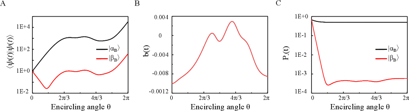
Without loss of generality, two cases are chosen as examples for demonstration. The encircling initial state is and for case I and case II, respectively. The start points of these two cases both locate at the -symmetry broken phase, and the encircling directions are all clockwise. Considering the Hamiltonian of the NV center, we multiply an overall coefficient of to the in equation (1) of the main text. The inner products of the encircling state, , are given in Supplementary Fig. S2A, where we can see that the inner products cover several orders of magnitude for both cases. The initial operators of were both set as when dilating into . The real value functions were both chosen as the form given in Supplementary Fig. S2B to keep operator positive during the dilation process. The probabilities of obtaining the ancilla qubit state , , are plotted in Supplementary Fig. S2C for both cases. Supplementary Fig. S2C shows that the in case I is big enough for measurement all the time. However, the in case II is only the magnitude of for some time and many repeat times of the experiment will be needed to measure it.
To reduce the difficulty of the experiment, we therefore introduce the measurement method in the main text. The dilated state of the two-qubit system in equation S2 can also be written as
| (S13) |
The state of the system qubit when the ancilla qubit state is is defined as
| (S14) |
We use quantum state tomography to measure state . Then state can be obtained by multiplying to state , renormalizing the state and finally using the maximum likelihood estimation PRA_Fiurasek_SM .
The four levels give rise to different photoluminescence(PL) rates PRB_Steiner_SM , labeled by , , , and , respectively. The PL rate differences can be used to readout the state of the two-qubit system. However, states with different population distributions can display the same PL rate, thus a set of pulse sequences given in Supplementary Fig. S3 were utilized to measure the dilated state.

The density matrix of the dilated state can be denoted by
| (S15) |
which means the density matrix of state is
| (S16) |
The first pulse sequence in Supplementary Fig. S3 represents direct readout of state , and the obtained PL rate was
| (S17) |
Similarly, we can write down the PL rates of the states after the effect of other pulses, this yields
| (S18) |
By solving equation S18, we can obtain that the elements of the density matrix are
| (S19) |
where , , and denote the PL rate differences between the corresponding energy levels. These PL rate differences were measured by Rabi oscillation experiments.
With equation S14, the density matrix of state can be calculated by
| (S20) |
where is a normalization coefficient, and the operator can be obtained from equation S6, that is .
The obtained density matrix may be non-physical. To solve this problem, a maximum likelihood estimation method is utilized to find the most possible physical state as the final .
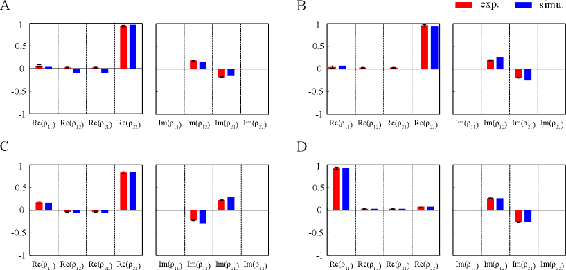
Supplementary Fig. S4 shows the results of the measured density matrix and the transformed density matrix by taking the case II as an example (Here we have replaced for t and the relation is ). The results of the encircling initial state are displayed in Supplementary Fig. S4A and B. The red bars are the experimental results and the blue bars are the simulation results which included the dephasing noise of the electron spin. The fidelities between the experimental obtained density matrixes and the simulated ones in Supplementary Fig. S4A and B are and , respectively. As for the encircling final state, the measured density matrix is depicted in Supplementary Fig. S4C and the transformed density matrix is given in Supplementary Fig. S4D. The fidelities between the experimental and simulated density matrixes in Supplementary Fig. S4C and D are and , respectively. For other encircling angles and each encircling cases, the fidelities between the experimental and simulated results are summarized in the Supplementary Table S1. The average fidelity between the experimental results and the simulated results for the measured density matrix and the transformed density matrix are both close to 1. These high fidelities show that the measured states agree well with the simulation predications.
| start point A | start point B | |||||||
| 0.98(4) | 1.00(5) | 1.00(2) | 0.99(3) | 1.00(4) | 0.97(3) | 1.00(4) | 0.98(3) | |
| 1.00(5) | 1.00(5) | 1.00(5) | 1.00(5) | 0.99(4) | 1.00(4) | 0.99(4) | 1.00(4) | |
| 0.96(3) | 0.98(4) | 0.96(3) | 0.97(3) | 0.97(2) | 0.99(2) | 0.99(1) | 0.99(3) | |
| 1.00(3) | 1.00(4) | 1.00(4) | 1.00(3) | 1.00(3) | 1.00(4) | 1.00(4) | 1.00(4) | |
| 0.99(3) | 0.99(3) | 0.98(3) | 0.96(2) | 0.99(1) | 0.98(1) | 1.00(1) | 0.99(3) | |
| 1.00(4) | 0.99(4) | 0.98(4) | 1.00(4) | 1.00(4) | 1.00(4) | 1.00(4) | 1.00(4) | |
| 0.96(1) | 0.99(3) | 0.97(4) | 0.98(1) | 0.97(1) | 1.00(1) | 0.99(1) | 0.96(3) | |
| 1.00(3) | 1.00(4) | 1.00(5) | 1.00(4) | 1.00(3) | 1.00(4) | 1.00(4) | 1.00(3) | |
| 1.00(1) | 0.97(3) | 0.99(1) | 0.97(1) | 0.99(1) | 0.99(5) | 0.97(2) | 0.98(3) | |
| 1.00(4) | 1.00(4) | 1.00(4) | 1.00(3) | 1.00(5) | 1.00(5) | 1.00(4) | 1.00(4) | |
| 0.99(2) | 0.99(1) | 0.99(1) | 0.98(1) | 0.98(2) | 0.99(1) | 0.98(1) | 0.98(2) | |
| 1.00(4) | 1.00(4) | 1.00(4) | 1.00(4) | 1.00(4) | 1.00(3) | 1.00(3) | 1.00(3) | |
| 0.99(1) | 1.00(1) | 0.99(3) | 0.99(1) | 0.98(1) | 0.99(1) | 0.99(1) | 0.99(1) | |
| 1.00(4) | 1.00(5) | 1.00(5) | 1.00(3) | 1.00(3) | 1.00(4) | 1.00(3) | 1.00(4) | |
IV Note IV: Construction of in the NV Center
This part demonstrates the construction of the dilated Hamiltonian in the NV center.
The dilated Hamiltonian we need to construct is
| (S21) |
The static Hamiltonian of the NV center has the form
| (S22) |
The subspace spanned by , , and is utilized to form a two-qubit system to perform the experiment. The static Hamiltonian of the NV center in this subspace can be simplified as
| (S23) |
To construct in this subspace, we apply two slightly detuned MW pulses to selectively drive the electron spin transitions, as depicted in Fig. 2b in the main text. The Hamiltonian of the pulses can be written as
| (S24) | ||||
where , and (, and ) are the amplitude, angular frequency and phase of the MW1 (MW2) pulse. Thus the total Hamiltonian of the NV center when applying MW pulses is
| (S25) | ||||
To construct in the NV center, we need to select an appropriate interaction picture and delicately set the parameters , , , , and .
Comparing the diagonal components of and , we can choose the interaction picture as
| (S26) |
The total Hamiltonian of the NV center in this interaction picture then transforms to
| (S27) | ||||
with () being the transition frequency between and ( and ). By choosing
| (S28) |
and in the condition of rotating wave approximation, we can simplify as
| (S29) | ||||
Comparing equation S29 with equation S21, if we choose
| (S30) |
then the dilated Hamiltonian can be realized.
References
- (1) Wu, Y. et al. Observation of parity-time symmetry breaking in a single spin system. Science 346, 878-880 (2019).
- (2) Fiurek, J., Maximum-likelihood estimation of quantum measurement. Phys. Rev. A. 64, 024102 (2001).
- (3) Steiner, M. et al. Universal Enhancement of the optical readout fidelity of single electron spins at nitrogen-vacancy centers in diamond. Phys. Rev. B 81, 035205 (2010).