Dynamically characterizing topological phases by high-order topological charges
Abstract
We propose a new theory to characterize equilibrium topological phase with non-equilibrium quantum dynamics by introducing the concept of high-order topological charges, with novel phenomena being predicted. Through a dimension reduction approach, we can characterize a -dimensional (D) integer-invariant topological phase with lower-dimensional topological number quantified by high-order topological charges, of which the th-order topological charges denote the monopoles confined on the th-order band inversion surfaces (BISs) that are D momentum subspaces. The bulk topology is determined by the th order topological charges enclosed by the th-order BISs. By quenching the system from trivial phase to topological regime, we show that the bulk topology of post-quench Hamiltonian can be detected through a high-order dynamical bulk-surface correspondence, in which both the high-order topological charges and high-order BISs are identified from quench dynamics. This characterization theory has essential advantages in two aspects. First, the highest (th) order topological charges are characterized by only discrete signs of spin-polarization in zero dimension (i.e. the th Chern numbers), whose measurement is much easier than the st-order topological charges that are characterized by the continuous charge-related spin texture in higher dimensional space. Secondly, a more striking result is that a first-order high integer-valued topological charge always reduces to multiple highest-order topological charges with unit charge value, and the latter can be readily detected in experiment. The two fundamental features greatly simplify the characterization and detection of the topological charges and also topological phases, which shall advance the experimental studies in the near future.
I Introduction
Topological quantum phases have become a mainstream of research in various areas, including condensed matter physics Klitzing et al. (1980); Tsui et al. (1982); Hasan and Kane (2010); Qi and Zhang (2011); Elliott and Franz (2015); Wen (2017); Kosterlitz (2017), ultracold atoms Greiner et al. (2002); Bloch et al. (2008); Miyake et al. (2013); Atala et al. (2013); Aidelsburger et al. (2013); Liu et al. (2014); Jotzu et al. (2014); Aidelsburger et al. (2015); Wu et al. (2016); Goldman et al. (2016); Lohse et al. (2018); Song et al. (2018), and photonic systems Verbin et al. (2013); Lu et al. (2016); Mittal et al. (2019). In equilibrium theory a topological phase is characterized by the bulk topological invariant defined in the ground state of the system and host protected boundary modes through the bulk-boundary correspondence. Based upon the equilibrium characterization the topological phases can be detected in experiment from the bulk-boundary correspondence, e.g. by resolving the boundary modes with angle-resolved photoelectron spectroscopy (ARPES) or transport measurements, which identify the equilibrium topological features König et al. (2007); Hsieh et al. (2008); Xia et al. (2009). The great success has been achieved in discovering the topological matter, such as topological insulators Fu et al. (2007); Fu and Kane (2007); Fu (2011); Chang et al. (2013), topological semimetals Burkov and Balents (2011); Young et al. (2012); Xu et al. (2015); Lv et al. (2015), and topological superconductors Qi et al. (2009); Bernevig and Hughes (2013); Ando and Fu (2015); Sato and Ando (2017); Zhang et al. (2018a).
Recently, as a momentum-space counterpart of the bulk-boundary correspondence, a dynamical bulk-surface correspondence was proposed for generic -dimensional (D) topological phases with integer invariants, and connects the bulk topology of such equilibrium topological phase and nontrivial dynamical pattern of quench-induced quantum dynamics emerging on the so-called band inversion surfaces (BISs) Zhang et al. (2018b, 2019a). The BISs are D interfaces in Brillouin zone (BZ) where the band inversion occurs, and are characterized by that the coupling between momentum and one (pseudo)spin component in the Hamiltonian vanishes Zhang et al. (2018b). By suddenly tuning the system from initially trivial phase to topological regime, the induced quench dynamics exhibit novel dynamical topological pattern on the D BISs, which is uniquely related to the bulk topology of the D equilibrium phase of the post-quench Hamiltonian. The dynamical bulk-surface correspondence establishes a universal correspondence between the equilibrium topological phases and far-from-equilibrium quantum dynamics. It provides conceptually new schemes to characterize and detect with high precision the equilibrium topological phases via non-equilibrium quench dynamics, which have been widely studied in the recent experiments with ultracold atoms Sun et al. (2018a, b); Yi et al. (2019); Song et al. (2019); Wang et al. , solid state spin systems Wang et al. (2019a); Ji et al. (2020); Xin et al. (2020), and superconducting circuits Niu et al. . Many novel issues have been further investigated in theory, such as the dynamical characterization of both symmetry-breaking order and topological phases in correlated systems Zhang et al. , the topological phases in non-Hermitian systems Zhou and Gong (2018); Qiu et al. (2019); Wang et al. (2019b); Zhu et al. (2020) and Floquet bands Zhang et al. (2020); Hu et al. (2020), generalization to generic quenches from a trivial or nontrivial phase via loop unitary construction Hu and Zhao (2020), and to the regime with slow nonadiabatic quantum quenches Ye and Li (2020). These studies also benefit from the high controllability of the synthetic quantum systems, which facilitates the exploration of non-equilibrium quantum dynamics Caio et al. (2015); Hu et al. (2016); Wang et al. (2017); Fläschner et al. (2018); Qiu et al. (2018); McGinley and Cooper (2019); Yang and Chen (2019); Tian et al. (2019); Xiong et al. (2020); Chen et al. (2020); Lu et al. (2020); Su et al. (2020).
The topology emerging on BISs can also be characterized by the topological charges enclosed in the BISs Zhang et al. (2019b), as an analogy to the Gaussian theorem, and such topological charges are dual to BISs and denote the monopole charges located at the nodes of the (pseudo)spin-orbit (SO) couplings Wang et al. (2019a); Ji et al. (2020); Yi et al. (2019). In this picture the topological invariant is viewed as the quantized flux of the monopoles through the BISs, which provides an intuitive perspective for the nontrivial bulk topology. More recently, the high-order BISs are proposed based on a dimension reduction approach Yu et al. , and the th-order BIS correspond to D momentum subspace which is reduced from -order BIS by further taking the coupling between momentum and the th (pseudo)spin component to be zero. In the quench dynamics the equilibrium topological phase can be characterized by the dynamical topology emerging on arbitrary high-order BISs. Since the higher-order BISs can be determined with less information, the dynamical theory based on high-order BISs can simplify the characterization of topological phases Yu et al. . The concept of high-order BIS is novelly extended by Li etal Li et al. to characterize the high-order topological phases Benalcazar et al. (2017a, b); Schindler et al. (2018). An interesting consideration is to extend the topological charges to the high-order regime based on the dimension reduction approach, which are dual to the high-order BISs and may have exceptional features and advantages in the dynamical characterization of topological phases, but have yet to be studied.
In this article, we introduce the concept of high-order topological charges, with which we propose a new dynamical characterization theory of topological phases. The equilibrium bulk topology is generically determined by the total th-order topological charges confined on the th-order BISs and enclosed in the th-order BISs. By quenching the system from trivial phase to topological regime, we further show that the topological phase of post-quench Hamiltonian can be detected through a high-order dynamical bulk-surface correspondence, in which both the high-order topological charges and high-order BISs are identified from quench dynamics. The proposed new characterization theory has two essential advantages: (i) Unlike the st-order topological charge whose characterization necessitates to measure the continuous charge-related (pseudo)spin texture in D space, which could be tedious, the highest (th) order topological charges are characterized by only discrete signs of spin-polarization in the zero dimension. (ii) A high integer-valued topological charge of the first order always reduces to multiple highest-order topological charges with unit charge value. Then the high integer-valued topological invariant can be read by the summation of the highest-order topological charges enclosed by the highest-order BISs. The two fundamental features greatly simplify the characterization and detection the equilibrium topological phases. Finally, these advantages of the dynamical characterization are illustrated with concrete examples.
The remaining part of this paper is organized as follows. In Sec. II, we introduce the generic theory of the new dynamical characterization. In Sec. III, our dynamical scheme is applied to two realistic models. In Sec. IV, we show the decomposition of high integer-valued topological charges. Finally, we summarize the main results and provide the brief discussion in Sec. V.
II Generic Theory
II.1 Model Hamiltonian and dimension reduction
We start with the basic Hamiltonian describing a -dimensional (D) gapped topological phase with integer invariant, which can be written in the elementary representation matrices of Clifford algebra Morimoto and Furusaki (2013); Chiu et al. (2016) as
| (1) |
where the vector field describes a D Zeeman field depending on the Bloch momentum in BZ. The matrices obey anti-commutation relations for , and their dimensionality is (or ) if is odd (or even), which is the minimal requirement to open a topological gap for the D topological phase. For 1D/2D case Su et al. (1980); Haldane (1988); Chiu et al. (2013), the matrices simply reduce to the Pauli matrices. For 3D/4D system Zhang and Hu (2001); Schnyder et al. (2008), the matrices are constructed as the tensor product of the Pauli matrices. The topology of this basic Hamiltonian is characterized by the D (or -th) winding number (or Chern number) if is odd (or even), which counts the coverage times of the mapping from the BZ torus to the D spherical surface Fruchart and Carpentier (2013).
Now we perform dimension reduction for the above Hamiltonian, and bulk topology will be reduced into the lower-dimensional subsystem. One can choose an arbitrary -component, say , to characterize the dispersion of the decoupled bands of . Accordingly, the remaining -components are denoted as the SO vector field . The SO vector field opens a topological gap at the band-crossing with , which is defined as the (first-order) BISs, namely . The bulk-surface duality has manifested that the bulk topology can be reduced to the winding of the D SO vector field on the D first-order BISs Zhang et al. (2018b). This lower-dimensional topology can be treated in an effective D gapped Hamiltonian on the first-order BISs,
| (2) |
where are the corresponding gamma matrices on the D subspace. The topological number of Hamiltonian (2) is given by the coverage times of the mapping from to . Now we can also define BISs for , which is called the second-order BISs Yu et al. . Without loss of generality, the component is used to define the D second-order BISs as . Then the bulk topology is reduced to the winding of the D effective SO vector field on the second-order BISs.
By repeating the above dimension reduction procedure, the D bulk topology can be reduced to the integer invariant of D effective Hamiltonian on the th-order BISs ,
| (3) |
where are the corresponding Gamma matrices on the D subspace. Thus component further defines the D th-order BISs as
| (4) |
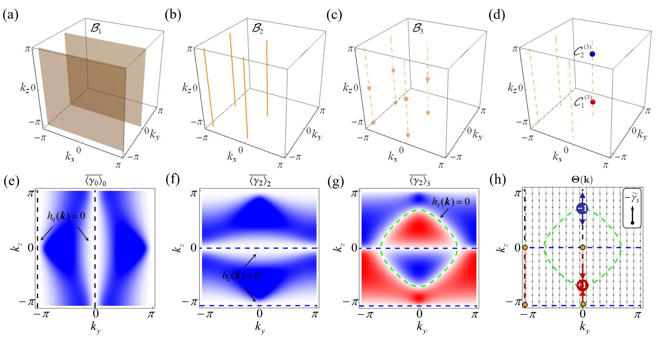
for [see Fig. 1(a)], and the remaining components represent the corresponding D effective SO vector field . The topological number is given by the winding of the D SO vector field on the th-order BISs [see Fig. 1(b)].
II.2 High-order topological charges
As an analogy to the Gaussian theorem, the bulk topology can also be characterized by the topological charges enclosed in the BISs, and such topological charges are dual to BISs and denote the monopole charges located at the nodes of the SO couplings Zhang et al. (2018b, 2019a, 2019b); Wang et al. (2019a); Ji et al. (2020); Yi et al. (2019). In this picture the topological invariant of is simply viewed as the quantized flux of the monopoles through the th-order BISs.

We introduce the th-order topological charges
| (5) |
which are located at the nodes of the D effective SO vector field with and characterize the corresponding monopoles. Here denotes a D interface on th-order BISs, enclosing the th monopole . In the typical case where is linear near the monopole, the th-order topological charges can be simplified as , where is Jacobian determinant with . However, when a monopole does not have the linear dispersion, the Jacobian is zero and the charge value is in fact larger than one.
We emphasize that the th-order topological charges are confined on the th-order BISs [see Fig. 1(a)] and are characterized by the all components of D effective SO vector field . Thus the properties (charge value and chirality) of th-order topological charges can be read out by measuring the (pseudo)spin structure of at in the (pseudo)spin subspace of coordinate system [see Fig. 1(c)]. In particular, one can find that the highest (th) order topological charges are only characterized by the discrete signs of at , i.e. the th Chern numbers Yu et al. . This intrinsic property determines that whose charge value is only . Moreover, a high integer-valued topological charge can always reduce to multiple highest-order topological charges with unit charge value by the dimension reduction procedure. This two fundamental features of highest-order topological charges can greatly simplify the characterization and detection the equilibrium topological phases, which avoids the redundant measurements of the continuous charge-related (pseudo)spin texture in high dimensional space and provides the easy measurements in experiments (See sections III and IV for details). This is one of the key ideas of this paper.
Besides, three points are worthwhile to mention: (i) The order of topological charge is actually the number of dimension reduction for bulk Hamiltonian. (ii) The real dimensionality for the arbitrary high-order topological charge is zero, because the topological charges are the nodes of effective SO vector field in momentum subspace. (iii) The configurations of high-order BISs are sharply different for choosing different -components of the Hamiltonian, thus the location of the corresponding high-order topological charges should be different. Nevertheless, this does not affect the results of topological characterization (see Appendix C).
II.3 High-order dynamical bulk-surface correspondence
We further propose to use quench dynamics to detect the high-order topological charges and the corresponding high-order BISs, which establishes the high-order dynamical bulk-surface correspondence to characterize the equilibrium topological phases. We consider a series of deep quench process (see Appendix A) along all axes with while only measure a single (pseudo)spin component , which is well measurable in cold atom experiments Sun et al. (2018a, b); Zhang et al. (2019a). Then the time-averaged (pseudo)spin polarization (TASP) is given by
| (6) |
where is the energy of the post-quenched Hamiltonian. Note that the TASP vanishes both on the momentum space with and .

Now the high-order topological charges and high-order BISs can be identified by measuring TASP. We define a set for , which includes the momenta with but . Then the closure also contains the momenta with . After setting , the vanishing TASP gives the th-order BISs when quenching the axes , i.e.
| (7) |
Correspondingly, the location of the th-order topological charges can be determined by the momenta . We further define the dynamical field
| (8) |
in (pseudo)spin subspace of coordinate system, where is a normalization factor and . Near the monopole charges, the dynamic field satisfies
| (9) |
whose (pseudo)spin structures intuitively give the properties of the th-order topological charges.
Finally, the bulk topology can be read out by the total th-order topological charges in the regions with enclosed by the th-order BISs, namely
| (10) |
The results of Eqs. (7)-(10) manifest a high-order dynamical bulk-surface correspondence, and provide the direct measurements of bulk topology via the well-resolved TASP in experiments. In addition, it is worth mentioning that we also provide another dynamical characterization scheme by quenching all (pseudo)spin axes and measuring multiple (pseudo)spin axis in Appendix C. Although the measurements of multiple (pseudo)spin components are challenging in recent experiments, this scheme is easier to determine high-order BISs and high-order topological charges, and then the equilibrium topological phase, which may has broader applications in the future.

III Application to the realistic models
We consider a simple D model with
| (11) |
which can be realized with recent advances. Here is the D momentum, and are the effective Zeeman coupling, and , are the nearest-neighbor spin-conserved and spin-flipped hopping coefficients, respectively.
The 2D quantum anomalous Hall (QAH) model with is considered first, which has been realized in cold atoms experiments Liu et al. (2014); Wu et al. (2016); Wang et al. (2018) and widely studied Zhang and Yi (2013); Pan et al. (2016); Liu et al. (2016); Poon and Liu (2018); Jia et al. (2019). The matrices are Pauli matrices . For , the bulk topology is characterized by the 1st Chern number (), where the topological phase corresponds to with , but the trivial phases are for with . We perform the quench by suddenly varying from to for , from to for , and from to for . The time evolution of spin polarization for -component only needs to be measured, which can present the second-order BISs and second-order topological charges and then gives the information of bulk topology.
A ring structure characterizes the first-order BIS with is observed from the vanishing TASP in Fig. 2(a). The vanishing polarization in Fig. 2(b) shows the surfaces of and , where the second-order BISs are given by on the first-order BIS and present two points when taking . Moreover, the second-order topological charges determined by sit on the first-order BIS and are obtained by the vanishing polarization , as shown in Fig. 2(c). Because the effective BZ is reduced as (or say ) and the bottom half-ring of first-order BIS holds , the second-order topological charge is enclosed into by the second-order BISs, which gives the 1st Chern number and is shown in Fig. 2(e). Compared with the dynamical characterization by using the first-order topological charges in Fig. 2(d), the spin textures around second-order topological charges are determined by the sign of at two sides of monopoles, which is more convenient for the experimental measurement.

We further consider the application to a 3D chiral topological insulator with , which has been simulated by using nitrogen-vacancy center Ji et al. (2020). The matrices are taken as , , , and , where and are both Pauli matrices. For , the topological phases are classified by the 3D winding number and are distinguished as: (i) with winding number ; (ii) with ; and (iii) with . Beyond these regions the phase is trivial. We perform the quench by suddenly varying from to for , from to for (tuning to and keeping ), then the bulk topology in region (i) can be read out by measuring the time evolution of pseudospin polarization of the -component.
The vanishing in six 2D planes of BZ implies , but the spherical-like surface is for , which identifies the first-order BIS [see Fig. 3(a)]. When taking the effective SO vector field as , the second-order BIS presents the ring-shape structure produced by in vanishing polarization of , which are confined on the first-order BIS [see Fig. 3(b)]. The corresponding second-order topological charges with are determined by the vanishing polarization of on the first-order BIS . The second-order topological charge is enclosed by the second-order BIS , giving the 3D winding number . Moreover, when the effective SO vector field is taken, the third-order BISs are produced by in vanishing polarization of , which are confined on the second-order BIS and present two points [see Fig. 3(c)]. The effective BZ is reduced as (or say ) and the front half-ring structure of the second-order BIS holds . Therefore, the 3D winding number is given by . Similarly, the observation of third-order topological charges are simpler to determine the bulk topology.
Particularly, here we can also identify the third-order topological charges by a minimum measurement scheme (see Appendix B) with advantage in future experiments. By measuring the TASP on some 2D planes of BZ, is for all momentum on the 2D plane of (The 2D plane of is failed to identify the third-order BISs ). Thus on this plane reflects the locations of the second-order BISs and third-order BISs [see Figs. 3(d1) and 3(d2)]. Therefore, the TASP and the normalized dynamic field on 2D plane of give the properties of the third-order topological charges and the topological number of the system [see Figs. 3(d3) and 3(d4)].

IV Decomposition of high integer-valued topological charges
For a monopole charge without linear dispersion, the charge value is larger than one and the system has a high-valued winding or Chern number. If detecting the topological charges with high charge value to identify the topological phases, it is cumbersome for the measurements of the continuous charge-related (pseudo)spin texture. Nevertheless, we can avoid these redundant measurements by reducing the high integer-valued topological charges to multiple highest-order topological charges with unit charge value. This essential advantage of the highest-order topological charge greatly simplifies topological characterization, especially for high-dimensional systems. Next we use two extended models to illustrate this point.
We first extend the 2D QAH model as follows:
| (12) |
with positive integer . For , the topological phase corresponds to with , but the trivial phase is still for . By quenching the system with in the same parameters as 2D QAH model, a ring-shape structure is identified as the first-order BIS from the vanishing polarization [see Fig. 4(a)]. Further, four first-order topological charges with high charge value are given by [see Fig. 4(b)]. Thus the bulk topology is determined by the summation of the first-order topological charges enclosed by the first-order BIS , i.e. [see Fig. 4(d)].
After taking for the dimension reduction, we observe the second-order BISs from the vanishing polarization , which is confined on the first-order BIS [see Fig. 4(b)]. Correspondingly, four second-order topological charges are obtained by the vanishing polarization [see Fig. 4(c)]. We emphasize that now each second-order topological charge has unit charge value , and then the bulk topology is calculated by the summation of second-order topological charges enclosed by the second-order BISs , i.e. [see Fig. 4(e)]. One can find that a first-order topological charge is separated into two second-order topological charges with unit negative charge by dimension reduction, and the total contribution of the remaining first-order topological charges is equivalent to two second-order topological charges with unit positive charge [see Fig. 4(f)]. The 2D topology with high integer-valued is transformed to 0D topology given by the summation of two 0th Chern numbers with , i.e. .
Similarly, we extend the 3D chiral topological insulator model as the following case,
| (13) |
For , the topological phases are classified by: (i) with ; (ii) with ; and (iii) with . By taking the quenched parameters as the same as 3D chiral topological insulator model, eight first-order topological charges with high charge value and a spherical-like first-order BIS [see Figs. 5(a) and 5(b)] can be observed by vanishing polarization of when taking . Thus the bulk topology is determined by the summation of first-order topological charges enclosed by the first-order BISs , i.e. .
After taking for the dimension reduction, six third-order topological charges sit on the second-order BISs [see Fig. 5(c)]. Each third-order topological charge has unit charge value , and then the bulk topology is given by the summation of third-order topological charges enclosed by the third-order BISs , i.e. [see Fig. 5(d)]. Similarly, a first-order topological charge is separated into three third-order topological charges with unit positive charge, and the total contribution of the remaining first-order topological charges is equivalent to the summation of three third-order topological charges with unit negative charge [see Fig. 5(e)]. Thus a high integer-valued D winding number with is transformed to the sum of three th Chern numbers, i.e. .
The above results strongly demonstrate the advantages of the highest-order topological charge in characterization of topological phases. Although the definition of topological charge depends on the selection of the -components, choosing a different -component to define the highest-order topological charge will not change the essence of its unit charge value, which is different from the first-order topological charge. Therefore, for a more general system, we only need to measure the properties of the highest-order topological charge to determine the bulk topology.
V Conclusion and discussion
In conclusion, we have proposed a new dynamical scheme to characterize the equilibrium topological phases based on the high-order topological charges, which correspond to monopoles confined in low dimensional subspaces. Through a dimensional reduction approach for a D bulk Hamiltonian, the topology of the D system can be determined by the arbitrary th order topological charges enclosed by the th-order BISs. In quenching the system from a trivial phase to a topologically nontrivial regime, both the high-order BISs and the high-order topological charges are directly observed by the quench induced (pseudo)spin dynamics, for which the topological phases of post-quench Hamiltonian can be detected dynamically.
The high-order topological charges have essential advantages in characterizing topological phases due to their intrinsic features. We compare the first-order and highest-order topological charges. For the first-order topological charge with unit or high charge value, as defined in D momentum space, its characterization generically necessitates to measure the continuous charge-related (pseudo)spin texture in D space. In comparison, the highest-order topological charges are defined in the zero dimension, and are characterized by the discrete signs of spin-polarization in zero dimension. This intrinsic feature determines that the charge value of a highest-order topological charge only takes . Accordingly, a high integer-valued lower-order topological charge can always reduce to multiple highest-order topological charges with unit charge value, which can be easily measured in experiment, hence simplifying the characterization and detection of topological phases.
ACKNOWLEDGEMENT
This work was supported by National Natural Science Foundation of China (Grants No. 11761161003, No. 11825401, and No. 11921005), the National Key R& D Program of China (Project No. 2016YFA0301604), Strategic Priority Research Program of the Chinese Academy of Science (Grant No. XDB28000000), and by the Open Project of Shenzhen Institute of Quantum Science and Engineering (Grant No.SIQSE202003).
Appendix A Deep quench process
In quenching the axis , we initialize a fully polarized state along the opposite axis by introducing a very large constant magnetization such that for . After , the magnetization is suddenly tuned to the topological regime, and the momentum-linked (pseudo)spin expectation will process around . The quantum dynamics is governed by the unitary evolution operator with the post-quenched Hamiltonian . We can measure the time-averaged (pseudo)spin polarization (TASP) of the component ,
| (14) |
where is the energy of the post-quenched Hamiltonian.
Appendix B Minimal measurement scheme
We provide a minimal dynamical scheme for the topological systems, in which the bulk topology is determined by the th-order topological charges enclosed by the D th-order BISs . This scheme greatly simplifies the characterization of bulk topological phases, especially for . We consider the topological systems with at least one plane-type component, say , which means that the momenta satisfying form planes. Note that both the th-order topological charges and the th-order BISs sit on the D th-order BISs consisting of momenta with . Since is plane-type, the th-order BISs also belong to the plane determined by . With these observations, to identify the th-order topological charges and the corresponding BISs, we can first extract the planes specified by from the TASP with vanishing values. On these planes, further determine the th order BISs . Finally, the th-order BISs and the th-order topological charges shall be found by observing and in the th BISs.

Appendix C Another dynamical characterization scheme
We provide another dynamical characterization scheme by quenching all (pseudo)spin axes and measuring multiple (pseudo)spin axis. On the other hand, we notice that the configurations of the high-order BISs and high-order topological charges are sharply different if choosing different components () of the Hamiltonian for definition. Here we take the different -components to define the high-order topological charges compared with the previous results.
We quench axes and measure the same axes for determination of th-order high-order BISs through TASP,
| (15) |
and then the th-order topological charges are identified by quenching the remaining axes and only measuring the component, i.e. with . We further define
| (16) |
in (pseudo)spin subspace with the coordinate system , where is a normalization factor. Near the monopole charge, the dynamic field satisfies , thus the high-order topological charge is determined directly by in the linear case. Note that the above dynamical characterization scheme is same with that in previous results for the determination of first-order topological charges. We next numerically examine the 2D QAH model and 3D chiral topological insulator model, and only consider the highest-order cases.
For 2D QAH model , we reselect
| (17) |
By quenching from to for and measuring the spin polarization of -component, the TASP is obtained. We observe that the first-order BISs are identified by , which are two lines in Fig. 6(a). Further, we quench the of system from to for and from to for . After only measuring the spin polarization of -component, the TASP are obtained. We observe that the second-order BISs present four points at , , , and , which are given by on the first-order BISs in Fig. 6(b). Finally, two second-order topological charges and at and are determined by of on the first-order BISs , as shown in Fig. 6(c). The bulk topology is determined by enclosed by the second-order BISs , i.e. .
We further consider the 3D chiral topological insulator model and reselect the component as follows:
| (18) |
where the matrices are taken as , , , and . When the quench is firstly performed by suddenly varying from to for and then the pseudospin polarization of -component is measured, we observe that the first-order BISs are identified by , which are two planes of and , as shown in Fig. 7(a). Secondly, we quench from to for and measure the pseudospin polarization of -component, the second-order BISs are identified by , which are four lines on the first-order BISs at and , as shown in Fig. 7(b). Thirdly, we quench from to for and from to for . By only measuring the pseudospin polarization of -component, the TASP are obtained. We observe that the third-order BISs present eight points given by on the second-order BISs , as shown in Fig. 7(c). Finally, two third-order topological charges and at and are determined by of on the second-order BISs , as shown in Fig. 7(d). Thus the bulk topology is determined by enclosed by the third-order BISs , i.e. .
Besides, we also give the 2D measurement to determine the bulk topology based on the minimal scheme of Appendix B. For this 3D model, the second-order BISs must be on 2D planes. One can measure the TASP on 2D planes after quench, then is for all on 2D planes of and . Therefore, the third-order BISs and the corresponding third-order topological charges are obtained by the TASP and , as shown in Figs. 7(e-g). The bulk topology is characterized by , as shown in Fig. 7(h).
References
- Klitzing et al. (1980) K. v. Klitzing, G. Dorda, and M. Pepper, Phys. Rev. Lett. 45, 494 (1980).
- Tsui et al. (1982) D. C. Tsui, H. L. Stormer, and A. C. Gossard, Phys. Rev. Lett. 48, 1559 (1982).
- Hasan and Kane (2010) M. Z. Hasan and C. L. Kane, Rev. Mod. Phys. 82, 3045 (2010).
- Qi and Zhang (2011) X.-L. Qi and S.-C. Zhang, Rev. Mod. Phys. 83, 1057 (2011).
- Elliott and Franz (2015) S. R. Elliott and M. Franz, Rev. Mod. Phys. 87, 137 (2015).
- Wen (2017) X.-G. Wen, Rev. Mod. Phys. 89, 041004 (2017).
- Kosterlitz (2017) J. M. Kosterlitz, Rev. Mod. Phys. 89, 040501 (2017).
- Greiner et al. (2002) M. Greiner, O. Mandel, T. Esslinger, T. W. Hänsch, and I. Bloch, Nature 415, 39 (2002).
- Bloch et al. (2008) I. Bloch, J. Dalibard, and W. Zwerger, Rev. Mod. Phys. 80, 885 (2008).
- Miyake et al. (2013) H. Miyake, G. A. Siviloglou, C. J. Kennedy, W. C. Burton, and W. Ketterle, Phys. Rev. Lett. 111, 185302 (2013).
- Atala et al. (2013) M. Atala, M. Aidelsburger, J. T. Barreiro, D. Abanin, T. Kitagawa, E. Demler, and I. Bloch, Nat. Phys. 9, 795 (2013).
- Aidelsburger et al. (2013) M. Aidelsburger, M. Atala, M. Lohse, J. T. Barreiro, B. Paredes, and I. Bloch, Phys. Rev. Lett. 111, 185301 (2013).
- Liu et al. (2014) X.-J. Liu, K. Law, and T. Ng, Phys. Rev. Lett. 112, 086401 (2014).
- Jotzu et al. (2014) G. Jotzu, M. Messer, R. Desbuquois, M. Lebrat, T. Uehlinger, D. Greif, and T. Esslinger, Nature 515, 237 (2014).
- Aidelsburger et al. (2015) M. Aidelsburger, M. Lohse, C. Schweizer, M. Atala, J. T. Barreiro, S. Nascimbène, N. Cooper, I. Bloch, and N. Goldman, Nat. Phys. 11, 162 (2015).
- Wu et al. (2016) Z. Wu, L. Zhang, W. Sun, X.-T. Xu, B.-Z. Wang, S.-C. Ji, Y. Deng, S. Chen, X.-J. Liu, and J.-W. Pan, Science 354, 83 (2016).
- Goldman et al. (2016) N. Goldman, J. C. Budich, and P. Zoller, Nat. Phys. 12, 639 (2016).
- Lohse et al. (2018) M. Lohse, C. Schweizer, H. M. Price, O. Zilberberg, and I. Bloch, Nature 553, 55 (2018).
- Song et al. (2018) B. Song, L. Zhang, C. He, T. F. J. Poon, E. Hajiyev, S. Zhang, X.-J. Liu, and G.-B. Jo, Sci. Adv. 4, eaao4748 (2018).
- Verbin et al. (2013) M. Verbin, O. Zilberberg, Y. E. Kraus, Y. Lahini, and Y. Silberberg, Phys. Rev. Lett. 110, 076403 (2013).
- Lu et al. (2016) L. Lu, J. D. Joannopoulos, and M. Soljačić, Nat. Phys. 12, 626 (2016).
- Mittal et al. (2019) S. Mittal, V. V. Orre, G. Zhu, M. A. Gorlach, A. Poddubny, and M. Hafezi, Nat. Photonics 13, 692 (2019).
- König et al. (2007) M. König, S. Wiedmann, C. Brüne, A. Roth, H. Buhmann, L. W. Molenkamp, X.-L. Qi, and S.-C. Zhang, Science 318, 766 (2007).
- Hsieh et al. (2008) D. Hsieh, D. Qian, L. Wray, Y. Xia, Y. S. Hor, R. J. Cava, and M. Z. Hasan, Nature 452, 970 (2008).
- Xia et al. (2009) Y. Xia, D. Qian, D. Hsieh, L. Wray, A. Pal, H. Lin, A. Bansil, D. Grauer, Y. S. Hor, R. J. Cava, et al., Nat. Phys. 5, 398 (2009).
- Fu et al. (2007) L. Fu, C. L. Kane, and E. J. Mele, Phys. Rev. Lett. 98, 106803 (2007).
- Fu and Kane (2007) L. Fu and C. L. Kane, Phys. Rev. B 76, 045302 (2007).
- Fu (2011) L. Fu, Phys. Rev. Lett. 106, 106802 (2011).
- Chang et al. (2013) C.-Z. Chang, J. Zhang, X. Feng, J. Shen, Z. Zhang, M. Guo, K. Li, Y. Ou, P. Wei, L.-L. Wang, et al., Science 340, 167 (2013).
- Burkov and Balents (2011) A. Burkov and L. Balents, Phys. Rev. Lett. 107, 127205 (2011).
- Young et al. (2012) S. M. Young, S. Zaheer, J. C. Teo, C. L. Kane, E. J. Mele, and A. M. Rappe, Phys. Rev. Lett. 108, 140405 (2012).
- Xu et al. (2015) S.-Y. Xu, I. Belopolski, N. Alidoust, M. Neupane, G. Bian, C. Zhang, R. Sankar, G. Chang, Z. Yuan, C.-C. Lee, et al., Science 349, 613 (2015).
- Lv et al. (2015) B. Lv, H. Weng, B. Fu, X. Wang, H. Miao, J. Ma, P. Richard, X. Huang, L. Zhao, G. Chen, et al., Phys. Rev. X 5, 031013 (2015).
- Qi et al. (2009) X.-L. Qi, T. L. Hughes, S. Raghu, and S.-C. Zhang, Phys. Rev. Lett. 102, 187001 (2009).
- Bernevig and Hughes (2013) B. A. Bernevig and T. L. Hughes, Topological insulators and topological superconductors (Princeton university press, 2013).
- Ando and Fu (2015) Y. Ando and L. Fu, Annu. Rev. Condens. Matter Phys. 6, 361 (2015).
- Sato and Ando (2017) M. Sato and Y. Ando, Rep. Prog. Phys. 80, 076501 (2017).
- Zhang et al. (2018a) P. Zhang, K. Yaji, T. Hashimoto, Y. Ota, T. Kondo, K. Okazaki, Z. Wang, J. Wen, G. Gu, H. Ding, et al., Science 360, 182 (2018a).
- Zhang et al. (2018b) L. Zhang, L. Zhang, S. Niu, and X.-J. Liu, Sci. Bull. 63, 1385 (2018b).
- Zhang et al. (2019a) L. Zhang, L. Zhang, and X.-J. Liu, Phys. Rev. A 100, 063624 (2019a).
- Sun et al. (2018a) W. Sun, B.-Z. Wang, X.-T. Xu, C.-R. Yi, L. Zhang, Z. Wu, Y. Deng, X.-J. Liu, S. Chen, and J.-W. Pan, Phys. Rev. Lett. 121, 150401 (2018a).
- Sun et al. (2018b) W. Sun, C.-R. Yi, B.-Z. Wang, W.-W. Zhang, B. C. Sanders, X.-T. Xu, Z.-Y. Wang, J. Schmiedmayer, Y. Deng, X.-J. Liu, et al., Phys. Rev. Lett. 121, 250403 (2018b).
- Yi et al. (2019) C.-R. Yi, L. Zhang, L. Zhang, R.-H. Jiao, X.-C. Cheng, Z.-Y. Wang, X.-T. Xu, W. Sun, X.-J. Liu, S. Chen, et al., Phys. Rev. Lett. 123, 190603 (2019).
- Song et al. (2019) B. Song, C. He, S. Niu, L. Zhang, Z. Ren, X.-J. Liu, and G.-B. Jo, Nat. Phys. 15, 911 (2019).
- (45) Z.-Y. Wang, X.-C. Cheng, B.-Z. Wang, J.-Y. Zhang, Y.-H. Lu, C.-R. Yi, S. Niu, Y. Deng, X.-J. Liu, S. Chen, et al., arXiv:2004.02413.
- Wang et al. (2019a) Y. Wang, W. Ji, Z. Chai, Y. Guo, M. Wang, X. Ye, P. Yu, L. Zhang, X. Qin, P. Wang, et al., Phys. Rev. A 100, 052328 (2019a).
- Ji et al. (2020) W. Ji, L. Zhang, M. Wang, L. Zhang, Y. Guo, Z. Chai, X. Rong, F. Shi, X.-J. Liu, Y. Wang, et al., Phys. Rev. Lett. 125, 020504 (2020).
- Xin et al. (2020) T. Xin, Y. Li, Y.-a. Fan, X. Zhu, Y. Zhang, X. Nie, J. Li, Q. Liu, and D. Lu, Phys. Rev. Lett. 125, 090502 (2020).
- (49) J. Niu, T. Yan, Y. Zhou, Z. Tao, X. Li, W. Liu, L. Zhang, S. Liu, Z. Yan, Y. Chen, et al., arXiv:2001.03933.
- (50) L. Zhang, L. Zhang, Y. Hu, S. Niu, and X.-J. Liu, arXiv:1903.09144.
- Zhou and Gong (2018) L. Zhou and J. Gong, Phys. Rev. B 98, 205417 (2018).
- Qiu et al. (2019) X. Qiu, T.-S. Deng, Y. Hu, P. Xue, and W. Yi, iScience 20, 392 (2019).
- Wang et al. (2019b) K. Wang, X. Qiu, L. Xiao, X. Zhan, Z. Bian, W. Yi, and P. Xue, Phys. Rev. Lett. 122, 020501 (2019b).
- Zhu et al. (2020) B. Zhu, Y. Ke, H. Zhong, and C. Lee, Phys. Rev. Research 2, 023043 (2020).
- Zhang et al. (2020) L. Zhang, L. Zhang, and X.-J. Liu, Phys. Rev. Lett. 125, 183001 (2020).
- Hu et al. (2020) H. Hu, B. Huang, E. Zhao, and W. V. Liu, Phys. Rev. Lett. 124, 057001 (2020).
- Hu and Zhao (2020) H. Hu and E. Zhao, Phys. Rev. Lett. 124, 160402 (2020).
- Ye and Li (2020) J. Ye and F. Li, Phys. Rev. A 102, 042209 (2020).
- Caio et al. (2015) M. Caio, N. R. Cooper, and M. Bhaseen, Phys. Rev. Lett. 115, 236403 (2015).
- Hu et al. (2016) Y. Hu, P. Zoller, and J. C. Budich, Phys. Rev. Lett. 117, 126803 (2016).
- Wang et al. (2017) C. Wang, P. Zhang, X. Chen, J. Yu, and H. Zhai, Phys. Rev. Lett. 118, 185701 (2017).
- Fläschner et al. (2018) N. Fläschner, D. Vogel, M. Tarnowski, B. Rem, D.-S. Lühmann, M. Heyl, J. Budich, L. Mathey, K. Sengstock, and C. Weitenberg, Nat. Phys. 14, 265 (2018).
- Qiu et al. (2018) X. Qiu, T.-S. Deng, G.-C. Guo, and W. Yi, Phys. Rev. A 98, 021601 (2018).
- McGinley and Cooper (2019) M. McGinley and N. R. Cooper, Phys. Rev. B 99, 075148 (2019).
- Yang and Chen (2019) C. Yang and S. Chen, Acta Phys. Sin. 68, 220304 (2019).
- Tian et al. (2019) T. Tian, Y. Ke, L. Zhang, S. Lin, Z. Shi, P. Huang, C. Lee, and J. Du, Phys. Rev. B 100, 024310 (2019).
- Xiong et al. (2020) Z. Xiong, D.-X. Yao, and Z. Yan, Phys. Rev. B 101, 174305 (2020).
- Chen et al. (2020) X. Chen, C. Wang, and J. Yu, Phys. Rev. A 101, 032104 (2020).
- Lu et al. (2020) Y.-H. Lu, B.-Z. Wang, and X.-J. Liu, Sci. Bull. 65, 2080 (2020).
- Su et al. (2020) K. Su, Z.-H. Sun, and H. Fan, Phys. Rev. A 101, 063613 (2020).
- Zhang et al. (2019b) L. Zhang, L. Zhang, and X.-J. Liu, Phys. Rev. A 99, 053606 (2019b).
- (72) X.-L. Yu, L. Zhang, J. Wu, and X.-J. Liu, arXiv:2004.14930.
- (73) L. Li, W. Zhu, and J. Gong, arXiv:2007.05759.
- Benalcazar et al. (2017a) W. A. Benalcazar, B. A. Bernevig, and T. L. Hughes, Science 357, 61 (2017a).
- Benalcazar et al. (2017b) W. A. Benalcazar, B. A. Bernevig, and T. L. Hughes, Phys. Rev. B 96, 245115 (2017b).
- Schindler et al. (2018) F. Schindler, A. M. Cook, M. G. Vergniory, Z. Wang, S. S. Parkin, B. A. Bernevig, and T. Neupert, Sci. Adv. 4, 0346 (2018).
- Morimoto and Furusaki (2013) T. Morimoto and A. Furusaki, Phys. Rev. B 88, 125129 (2013).
- Chiu et al. (2016) C.-K. Chiu, J. C. Teo, A. P. Schnyder, and S. Ryu, Rev. Mod. Phys. 88, 035005 (2016).
- Su et al. (1980) W.-P. Su, J. Schrieffer, and A. Heeger, Phys. Rev. B 22, 2099 (1980).
- Haldane (1988) F. D. M. Haldane, Phys. Rev. Lett. 61, 2015 (1988).
- Chiu et al. (2013) C.-K. Chiu, H. Yao, and S. Ryu, Phys. Rev. B 88, 075142 (2013).
- Zhang and Hu (2001) S.-C. Zhang and J. Hu, Science 294, 823 (2001).
- Schnyder et al. (2008) A. P. Schnyder, S. Ryu, A. Furusaki, and A. W. Ludwig, Phys. Rev. B 78, 195125 (2008).
- Fruchart and Carpentier (2013) M. Fruchart and D. Carpentier, C. R. Phys. 14, 779 (2013).
- Wang et al. (2018) B.-Z. Wang, Y.-H. Lu, W. Sun, S. Chen, Y. Deng, and X.-J. Liu, Phys. Rev. A 97, 011605 (2018).
- Zhang and Yi (2013) W. Zhang and W. Yi, Nat. Commun. 4, 2711 (2013).
- Pan et al. (2016) J.-S. Pan, W. Zhang, W. Yi, and G.-C. Guo, Phys. Rev. A 94, 043619 (2016).
- Liu et al. (2016) X.-J. Liu, Z.-X. Liu, K. T. Law, W. V. Liu, and T. K. Ng, New J. Phys. 18, 035004 (2016).
- Poon and Liu (2018) T. F. J. Poon and X.-J. Liu, Phys. Rev. B 97, 020501 (2018).
- Jia et al. (2019) W. Jia, Z.-H. Huang, X. Wei, Q. Zhao, and X.-J. Liu, Phys. Rev. B 99, 094520 (2019).