Dynamical Generation of Epsilon-Near-Zero Behaviour via Tracking and Feedback Control

One of the principal research goals of the twenty first century optics has been the development and application of epsilon-near-zero (ENZ) materials. These form a subclass of near zero index (NZI) materials, whose common feature is the extraordinary optical properties they possess [1, 2, 3, 4, 5, 6]. Such materials exhibit a near zero permittivity or permeability at a given frequency, leading to a decoupling of the electric and magnetic fields [3, 4, 7, 2, 8]. Such behaviour has exceptional potential to further our capabilities in the generation and manipulation of nonlinear optical effects at the nanoscale [9], and represent a vital element in many proposed quantum technologies. For example, ENZ materials can be used to control the phase and direction of emission in antennas [10, 11, 12], while in optical circuits, the can behave effectively as components such as switches [13, 14, 15, 16, 17, 18] and modulators [19, 20, 21, 22, 23, 24, 25].

To date, experimental realization of these materials is primarily achieved through the construction of artificially constructed metamaterials [26, 27, 28, 29, 30, 31, 32, 33, 34] and at the plasma frequency in materials with a Drude dispersion relation [35, 36, 37, 38, 39, 40, 41, 42, 43]. Though convenient and compatible with complementary metal oxide semiconductor (CMOS) devices [1], there are large intrinsic loses in the metals and semiconductors in which irradiation at the plasma frequency induces an ENZ response [3]. This is precisely a consequence of the definitional property of an ENZ, namely its near-zero dielectric permittivity [44]. Moreover, the bandwidth of current metamaterials is narrow, limiting ENZ metamaterials’ usefulness in real-world applications [45, 46, 47, 48]. Recent work has shown however that coupling metamaterials to circuits with negative reactance, so-called non-Foster circuits [49], can increase their bandwidth and ameliorate this issue [45, 50, 51].

Given the current limitations of metamaterial design and fabrication, one might ask if there is an alternative route to achieving the sought-for optical properties exhibited by an ENZ material. Since this behaviour characterises the response of a material to optical driving, an alternative to engineering the equilibrium properties of materials might be to instead consider how the relationship between driving and response can characterised and manipulated. Specifically, we ask whether an ENZ-like response be generated dynamically by designing a driving field whose response functionally emulates that expected from an ENZ, namely an infinite phase velocity.

To achieve this objective, it is necessary to import techniques from the field of quantum control [52, 53]. In particular, tracking control [54, 55, 56, 57, 58, 59, 60, 61] provides a method for calculating driving fields such that the evolution of a given observable tracks a specified trajectory. These methods have been deployed profitably in the context of atomic [57], molecular [55, 62, 63] and solid-state systems [60, 61, 64, 65]. Complementary to this method is feedback control [66]. This has been implemented in a wide variety of systems for applications ranging from cruise control [67, 68, 69] to computer network protocols [70, 71, 72, 73] and atomic force microscopy [74, 75]. Recently the concept of feedback control has been further extended into the realm of quantum algorithm optimisation [76, 77], but to date has not been applied to the manipulation of quantum system’s nonlinear optical properties.

In this letter, we demonstrate that using either tracking or feedback control allows for the dynamical generation of an ENZ response in a many-body system. Furthermore, we show that this behaviour mimics that of an ideal inductor, raising the possibility that feedback control mechanisms can be used to create optical analogues to the fundamental components of electrical circuitry. Significantly, the proposed method admits the possibility of negative inductances, furnishing precisely the type of non-Foster behaviour necessary for increasing the bandwidth of metamaterials.

We begin by outlining the procedure for tracking control, and detail how this is applied to generate an ENZ response in a many-body system. We consider a one-dimensional model throughout this letter for the sake of simplicity, but the following analysis can be generalized to higher dimensions. We take as a model a general many-body fermionic system in which $N_{e}$ electrons are localized to lattice sites $j=1,...,N_{s}$ with spin $\sigma=\uparrow,\downarrow$. The kinetic energy is described by the hopping parameter $t_{0}$, acting as an effective single band system coupled to a driving laser via the dipole approximation. The effect of this is to introduce a phase $\exp[\pm i\Phi(t)]$ onto the hopping parameter, where $\Phi(t)$ is the Peierls phase [78, 79]. The Hamiltonian is then described by (in atomic units):

$$\hat{H}(t)=-t_{0}\sum_{j,\sigma}\left(e^{-i\Phi(t)}\hat{c}^{\dagger}_{j,\sigma}\hat{c}_{j+1,\sigma}+\mathrm{h.c.}\right)+\hat{U}$$

(1)

where $\hat{c}^{{\dagger}}_{j,\sigma}$ and $\hat{c}_{j,\sigma}$ are, respectively, the canonical fermionic creation and annihilation operators, and $\hat{U}$ describes the potential resulting from electron-electron repulsion.

Optical driving induces a current in the system which is calculated by the expectation of the current operator. The current operator is derived by a continuity equation [60, 61, 64], giving:

$$\hat{J}(t)=-iat_{0}\sum_{j,\sigma}\left(e^{-i\Phi(t)}\hat{c}^{\dagger}_{j,\sigma}\hat{c}_{j+1,\sigma}-\mathrm{h.c.}\right)$$

(2)

where $a$ is the lattice constant. The optical emission of a driven material is determined exclusively by this current, and forms the basis for the study of optical response in the solid state [80, 81, 82, 83]. This is due to the fact that under the dipole approximation, the emitted field is proportional to the dipole acceleration $\frac{dJ(t)}{dt}$, where $J(t)\equiv\langle\psi(t)|\hat{J}(t)|\psi(t)\rangle$. For this reason, it is via the control of this observable that an ENZ response can be generated.

The condition for an ENZ response can be formulated in terms of the relationship between the driving field and response. The infinite phase velocity implied by a near-zero dielectric permittivity implies a zero lag between the applied and emitted electrical fields, i.e. $E_{\mathrm{out}}(t)\propto E_{\mathrm{in}}(t)$. This relationship can be expressed in terms of $\Phi(t)$ and $J$ by recalling that $E_{\mathrm{in}}(t)=-\frac{1}{a}\frac{d\Phi(t)}{dt}$ [60]. Thus, the ENZ criteria can be succinctly represented by

$$\frac{\mathrm{d}J(t)}{\mathrm{d}t}=-\frac{1}{a\mathfrak{L}}\frac{\mathrm{d}\Phi(t)}{\mathrm{d}t},$$

(3)

where $\mathfrak{L}$ is a non-zero real constant. Integrating both sides with respect to time, we obtain a condition for an ENZ response $J_{\rm ENZ}$,

$$J_{\rm ENZ}(t)=-\frac{1}{a\mathfrak{L}}\Phi_{\rm ENZ}(t)+C$$

(4)

which can be implemented directly in a tracking control framework.

The laser field $-\frac{1}{a}d\Phi_{\rm ENZ}(t)/dt$ that induces an ENZ response is given by the solution to the implicit equation

$$\begin{split}\frac{1}{a\mathfrak{L}}\Phi_{\rm ENZ}(\psi)=2at_{0}R(\psi)\sin\left[\Phi_{\rm ENZ}(\psi)-\theta(\psi)\right]+J(0).\end{split}$$

(5)

Here, $J(0)$ is the current expectation of the initial state, and $R(\psi)$ and $\theta(\psi)$ are, respectively, the real and imaginary components of the nearest neighbor expectation $\langle\sum_{j,\sigma}\hat{c}^{\dagger}_{j,\sigma}\hat{c}_{j+1,\sigma}\rangle$. The derivation of Eq. (5) is provided in Sec. I of the supplemental materials, and the existence of such a field and the conditions under which it is unique are demonstrated in Sec. II [84]. Finally, it is worth noting that the physical validity of this tracking equation in the $\mathrm{d}t\rightarrow 0$ limit can be checked by comparison to the Ehrenfest theorem for $J(t)$ (see e.g. [61]).

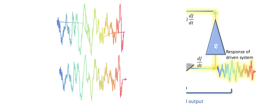
An alternative route to obtaining an ENZ response can be obtained by using the material’s own response to control the input field. Here, we implement a simple form of feedback control known as proportional feedback control, a schematic for which is given in Fig. 1. In this scenario, we begin by applying a transform limited pulse with electric field $E_{\rm tl}(t)$ which is subsequently modified by the introduction of the control field

$$u(t)=k_{p}\left(\mathfrak{L}\frac{\mathrm{d}J(t)}{\mathrm{d}t}-E_{\rm in}(t)\right)$$

(6)

where $k_{p}$ is a positive constant representing the amplification gain. The control field enforces the ENZ condition (3) by correcting the input field when the error $e=\mathfrak{L}\frac{\mathrm{d}J}{dt}-E_{\rm in}$ is nonzero.

The combined input to the system when we correct the transform limited field with the control field (6) is then

$$E_{\rm in}(t)=E_{\rm tl}(t)+u(t).$$

(7)

Substituting $E_{\rm in}(t)$ as given above into Eq. (6) together with some algebraic rearrangement allows us to express it as

$$u(t)=\frac{k_{p}}{1+k_{p}}\left(\mathfrak{L}\frac{\mathrm{d}J(t)}{\mathrm{d}t}-E_{\rm tl}(t)\right),$$

(8)

which in the limit $k_{p}\rightarrow\infty$, gives $u(t)=\mathfrak{L}\frac{\mathrm{d}J(t)}{\mathrm{d}t}-E_{\rm tl}(t)$. Then, by Eq. (7), the input field approaches

$$E_{\rm in}(t)\to E_{\rm ENZ}(t)=\mathfrak{L}\frac{\mathrm{d}J(t)}{\mathrm{d}t},$$

(9)

the ENZ condition. Hence, given sufficiently strong amplification $k_{p}$, the feedback scheme Fig. 1 will drive any system to produce ENZ response.

To computationally illustrate this, we calculate the Peierls phase by multiplying Eq. (7) by $-a$ and integrating over time:

$$\Phi_{\rm in}(t)=\Phi_{\rm tl}(t)+\frac{k_{p}}{1+k_{p}}\left[-a\mathfrak{L}\left(J(t)-J(0)\right)-\Phi_{\rm tl}(t)\right].$$

(10)

A natural question is how the free parameter $\mathfrak{L}$ should be interpreted. When considering Eq. (3), it bears a strong resemblance to the dynamics of an inductor [85]. For an inductor with intrinsic inductance $L$ and length $d$ subject to a homogeneous time dependent electric field $E(t)$, we have

$$\frac{\mathrm{d}I(t)}{\mathrm{d}t}=\frac{d}{L}E(t)$$

(11)

Here, $I(t)$ is the macroscopic current which varies only in time. The total energy $\mathcal{E}$ stored by an inductor at time $t$ is

$$\mathcal{E}(t)-\mathcal{E}(0)=\frac{L}{2}\left[I^{2}(t)-I^{2}(0)\right].$$

(12)

In the scenario we consider, the dynamics take place on the nanoscale, so we substitute the macroscopic current for the current expectation $J(x,t)=\langle\hat{J}(x,t)\rangle$. Then, we discretise with $J(x,t)\rightarrow\frac{1}{a}J_{j}(t)$ and $\int\mathrm{d}x\rightarrow a\sum_{j}$ to obtain the relationship between energy and current in a system defined by Eq. (1). The power stored by the solid-state system will be

$$P(t)=E(t)\sum_{j}J_{j}(t)=E(t)J(t),$$

(13)

which after time integration yields

$$\mathcal{E}(t)-\mathcal{E}(0)=-\frac{1}{a}\int_{0}^{t}\frac{{\rm d}\Phi(t^{\prime})}{{\rm d}t^{\prime}}J(t^{\prime})\mathrm{d}t^{\prime}.$$

(14)

Upon inserting the specific form of $\Phi(t)$ imposed by the ENZ condition given in Eq. (4), we obtain an identical energy-current relationship to that of the inductor shown in Eq. (12):

$$\mathcal{E}(t)-\mathcal{E}(0)=\frac{\mathfrak{L}}{2}\left[J^{2}(t)-J^{2}(0)\right],$$

(15)

and hence we are able to identify the value of $\mathfrak{L}$ chosen as an effective inductance.

We now demonstrate that both tracking and feedback control induce the desired ENZ response via numerical calculations. Though the Hamiltonian in Eq. (1) and subsequent analysis of the field required to induce an ENZ response are valid for any $\hat{U}$ that will commute with electron number operators [64, 65], for simulations we take our system to be a half-filled Fermi-Hubbard model ($N_{s}=N_{e}$) [86], where $N_{\uparrow}=N_{\downarrow}$ and onsite interaction of the form

$$\hat{U}=U\sum_{j=1}^{N}\hat{n}_{j,\uparrow}\hat{n}_{j,\downarrow}$$

(16)

where $U$ parametrises interaction energy and $\hat{n}_{j,\sigma}=\hat{c}^{\dagger}_{j,\sigma}\hat{c}_{j,\sigma}$ is the number operator for site $j$ and spin $\sigma$.

Numerical simulations of both types of control are performed using the QuSpin package in Python [87]. To avoid trivial solutions of zero field and current, after initialising the simulation in the ground state of the system, we then excite it with 10 cycles of a transform limited pump pulse of strength $F_{0}=10\frac{\mathrm{MV}}{\mathrm{cm}}$ and frequency $\omega_{0}=32.9$ THz. After this pre-pump, we implement the chosen control procedure. The system is evolved using the DOP853 algorithm [88] implemented in SciPy [89] for a total time equal to the duration of the pump pulse $T=\frac{2\pi M}{\omega_{0}}$ where $M$ is the number of cycles. At each time step, we solve Eq. (5) for tracking control and Eq. (10) for feedback control.

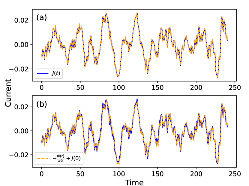
A specific example of tracking and feedback control is shown in Fig. 2. Most importantly, when $\left|2a^{2}t_{0}N_{s}\mathfrak{L}\right|\leq 1$ we expect the ENZ response to be unique (see Sec. II of the supplemental material [84]), and consequently we find that both feedback and tracking control yield identical solutions. Note that the derived driving field exhibits a high degree of complexity and bandwidth, which would be challenging to reproduce with current pulse shaping technology. There is a real prospect, however, of controlling the input electric field using the materials own response via feedback control.

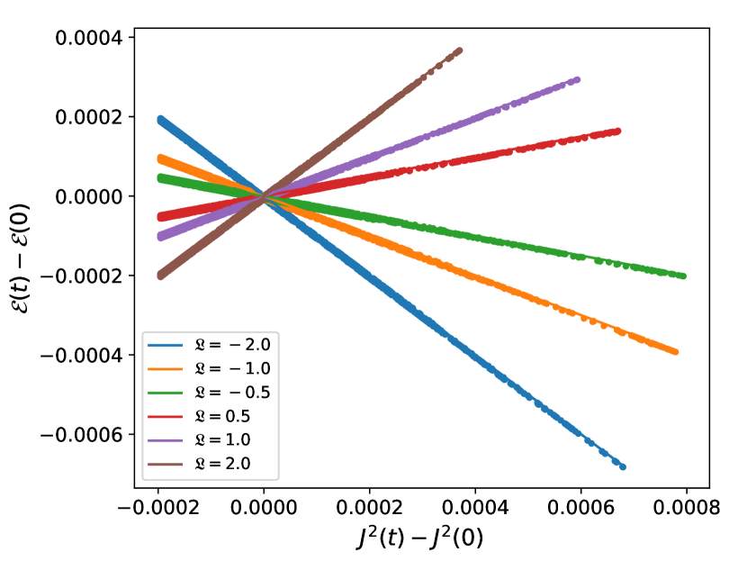
As predicted by Eq. (15) and demonstrated in Fig. 3, the relationship between the change in energy and the change in the square of the current is exactly linear and the slope increases with increasing $\mathfrak{L}$. The relationship holds for positive as well as negative values of $\mathfrak{L}$, and thus allows us to induce a non-Foster response by specifying $\mathfrak{L}<0$.

In this letter, we have demonstrated the possibility of inducing an ENZ response in a large class of solid-state systems using either tracking or feedback control. Tracking control gives extremely precise control over the induced current, but faces significant hurdles to practical implementation due to the bandwidth of driving pulses. In contrast, feedback control replaces pulse shaping with amplification, and can therefore be implemented relatively straightforwardly. In the current work, we have assumed an instantaneous feedback, but this can easily be adapted to a finite optical path by preparing two identical copies of the system, and using feeding the response of one system to the initial pulse into the input of the second at a suitable time delay. Given the equivalence in the solutions they predict, it is possible that the most direct route to implementing many tracking control proposals will be to adapt them to a feedback procedure. It is also worth noting that the particular response one obtains from tracking will depend on the initial state, and hence the specific pump profile one applies before tracking. This offers a route to tailoring the response obtained. For example, one could generate a maximum or minimum bandwidth for the response by performing an optimisation over pump pulse parameters, conditioned on the desired property.

The equations developed here allow one to tune the scaling of the system response relative to the input field by a factor $\mathfrak{L}$. Analytically, this parameter is shown to be analogous to macroscopic inductance (15), and we demonstrate that the predicted energy-current relationship is realized in simulations in Fig. 3. There are no restrictions on the sign of this inductance can take, meaning it is possible to specify $\mathfrak{L}<0$ to induce a non-Foster reactance. Since coupling negative inductance materials to metamaterials has been shown to increase metamaterials’ bandwidth, not only can we drive an ENZ response in these materials, but optical feedback control may offer an indirect route to realising ENZ behaviour in metamaterials by broadening their bandwidth.

The mapping between the ENZ response and an ideal inductor also hints at the possibility that feedback control may be employed to develop quantum optical analogs to other basic components of classical electrical circuits, such as resistance and capacitance. The possibility of an all optical computation has already been demonstrated in [90], and with the limit of Moore’s law being approached [91], the need for alternative computing platforms is pressing. Optical feedback control therefore represents a potential opportunity to take advantage of the inherent nonlinearities present in quantum optics, in order to develop computing at the nanoscale.

Acknowledgement. This work was supported by the W. M. Keck Foundation and by Army Research Office (ARO) (grant W911NF-19-1-0377, program manager Dr. James Joseph, and cooperative agreement W911NF-21-2-0139). The views and conclusions contained in this document are those of the authors and should not be interpreted as representing the official policies, either expressed or implied, of ARO or the U.S. Government. The U.S. Government is authorized to reproduce and distribute reprints for Government purposes notwithstanding any copyright notation herein.

References

- Wu et al. [2021] J. Wu, Z. T. Xie, Y. Sha, H. Y. Fu, and Q. Li, Epsilon-near-zero photonics: infinite potentials, Photon. Res. 9, 1616 (2021).
- Ziolkowski [2004] R. W. Ziolkowski, Propagation in and scattering from a matched metamaterial having a zero index of refraction, Physical Review E 70, 046608 (2004).
- Niu et al. [2018] X. Niu, X. Hu, S. Chu, and Q. Gong, Epsilon-near-zero photonics: A new platform for integrated devices, Advanced Optical Materials 6, 1701292 (2018), https://onlinelibrary.wiley.com/doi/pdf/10.1002/adom.201701292 .
- Liberal and Engheta [2017a] I. Liberal and N. Engheta, Near-zero refractive index photonics, Nature Photonics 11, 149 (2017a).
- Liberal and Engheta [2017b] I. Liberal and N. Engheta, The rise of near-zero-index technologies, Science 358, 1540 (2017b), https://www.science.org/doi/pdf/10.1126/science.aaq0459 .
- Kinsey et al. [2019] N. Kinsey, C. DeVault, A. Boltasseva, and V. M. Shalaev, Near-zero-index materials for photonics, Nature Reviews Materials 4, 742 (2019).
- Engheta and Ziolkowski [2006] N. Engheta and R. W. Ziolkowski, Metamaterials: physics and engineering explorations (John Wiley & Sons, 2006).
- Engheta [2013] N. Engheta, Pursuing near-zero response, Science 340, 286 (2013).
- Vincenti et al. [2020] M. A. Vincenti, D. de Ceglia, and M. Scalora, ENZ materials and anisotropy: enhancing nonlinear optical interactions at the nanoscale, Opt. Express 28, 31180 (2020).
- Tong et al. [2020] S. Tong, C. Ren, J. Tao, and W. Tang, Anisotropic index-near-zero metamaterials for enhanced directional acoustic emission, Journal of Physics D: Applied Physics 53, 265102 (2020).
- Vlasov et al. [2001] Y. A. Vlasov, X.-Z. Bo, J. C. Sturm, and D. J. Norris, On-chip natural assembly of silicon photonic bandgap crystals, Nature 414, 289 (2001).
- Enoch et al. [2002] S. Enoch, G. Tayeb, P. Sabouroux, N. Guérin, and P. Vincent, A metamaterial for directive emission, Phys. Rev. Lett. 89, 213902 (2002).
- Guo et al. [2017] Q. Guo, Y. Cui, Y. Yao, Y. Ye, Y. Yang, X. Liu, S. Zhang, X. Liu, J. Qiu, and H. Hosono, A solution-processed ultrafast optical switch based on a nanostructured epsilon-near-zero medium, Advanced Materials 29, 1700754 (2017), https://onlinelibrary.wiley.com/doi/pdf/10.1002/adma.201700754 .
- Xie et al. [2020] Z. T. Xie, J. Wu, H. Y. Fu, and Q. Li, Tunable electro- and all-optical switch based on epsilon-near-zero metasurface, IEEE Photonics Journal 12, 1 (2020).
- Bohn et al. [2021] J. Bohn, T. S. Luk, C. Tollerton, S. W. Hutchings, I. Brener, S. Horsley, W. L. Barnes, and E. Hendry, All-optical switching of an epsilon-near-zero plasmon resonance in indium tin oxide, Nature Communications 12, 1017 (2021).
- Kuttruff et al. [2020] J. Kuttruff, D. Garoli, J. Allerbeck, R. Krahne, A. De Luca, D. Brida, V. Caligiuri, and N. Maccaferri, Ultrafast all-optical switching enabled by epsilon-near-zero-tailored absorption in metal-insulator nanocavities, Communications Physics 3, 114 (2020).
- Zhang et al. [2020] C. Zhang, Y. Zu, W. Yang, S. Jiang, and J. Liu, Epsilon-near-zero medium for optical switches in ho solid-state laser at 2.06 μm, Optics & Laser Technology 129, 106271 (2020).
- Zhang et al. [2019] Z. Zhang, J. Liu, Q. Hao, and J. Liu, Sensitive saturable absorber and optical switch of epsilon-near-zero medium, Applied Physics Express 12, 065504 (2019).
- Lu et al. [2012] Z. Lu, W. Zhao, and K. Shi, Ultracompact electroabsorption modulators based on tunable epsilon-near-zero-slot waveguides, IEEE Photonics Journal 4, 735 (2012).
- Zhao et al. [2015] H. Zhao, Y. Wang, A. Capretti, L. D. Negro, and J. Klamkin, Broadband electroabsorption modulators design based on epsilon-near-zero indium tin oxide, IEEE Journal of Selected Topics in Quantum Electronics 21, 192 (2015).
- Koch et al. [2016] U. Koch, C. Hoessbacher, J. Niegemann, C. Hafner, and J. Leuthold, Digital plasmonic absorption modulator exploiting epsilon-near-zero in transparent conducting oxides, IEEE Photonics Journal 8, 1 (2016).
- Baek et al. [2015] J. Baek, J.-B. You, and K. Yu, Free-carrier electro-refraction modulation based on a silicon slot waveguide with ito, Opt. Express 23, 15863 (2015).
- Lee et al. [2014] H. W. Lee, G. Papadakis, S. P. Burgos, K. Chander, A. Kriesch, R. Pala, U. Peschel, and H. A. Atwater, Nanoscale conducting oxide plasmostor, Nano Letters 14, 6463 (2014).
- Vasudev et al. [2013] A. P. Vasudev, J.-H. Kang, J. Park, X. Liu, and M. L. Brongersma, Electro-optical modulation of a silicon waveguide with an “epsilon-near-zero” material, Opt. Express 21, 26387 (2013).
- Liu et al. [2018] X. Liu, K. Zang, J.-H. Kang, J. Park, J. S. Harris, P. G. Kik, and M. L. Brongersma, Epsilon-near-zero si slot-waveguide modulator, ACS Photonics 5, 4484 (2018).
- Rizza et al. [2011] C. Rizza, A. Di Falco, and A. Ciattoni, Gain assisted nanocomposite multilayers with near zero permittivity modulus at visible frequencies, Applied Physics Letters 99, 221107 (2011), https://doi.org/10.1063/1.3665414 .
- Maas et al. [2013] R. Maas, J. Parsons, N. Engheta, and A. Polman, Experimental realization of an epsilon-near-zero metamaterial at visible wavelengths, Nature Photonics 7, 907 (2013).
- Zhao and Xie [2019] L. Zhao and H. Xie, A novel optical \textepsilon-near-zero material realized by multi-layered ag/sic film structures, Optik 183, 513 (2019).
- Kelley et al. [2019] K. P. Kelley, E. L. Runnerstrom, E. Sachet, C. T. Shelton, E. D. Grimley, A. Klump, J. M. LeBeau, Z. Sitar, J. Y. Suen, W. J. Padilla, and J.-P. Maria, Multiple epsilon-near-zero resonances in multilayered cadmium oxide: Designing metamaterial-like optical properties in monolithic materials, ACS Photonics 6, 1139 (2019).
- Dai and Zhang [2015] D. Dai and M. Zhang, Mode hybridization and conversion in silicon-on-insulator nanowires with angled sidewalls, Opt. Express 23, 32452 (2015).
- Caligiuri et al. [2019] V. Caligiuri, M. Palei, G. Biffi, and R. Krahne, Nanophotonics 8, 1505 (2019).
- Rashed et al. [2020] A. R. Rashed, B. C. Yildiz, S. R. Ayyagari, and H. Caglayan, Hot electron dynamics in ultrafast multilayer epsilon-near-zero metamaterials, Phys. Rev. B 101, 165301 (2020).
- Koivurova et al. [2020] M. Koivurova, T. Hakala, J. Turunen, A. T. Friberg, M. Ornigotti, and H. Caglayan, Metamaterials designed for enhanced enz properties, New Journal of Physics 22, 093054 (2020).
- Lee and Kee [2021] Y. G. Lee and C.-S. Kee, Constant cutoff frequency of a two-dimensional photonic crystal composed of metallic rods and epsilon-near-zero materials, Physica B: Condensed Matter 600, 412598 (2021).
- Anderegg et al. [1971] M. Anderegg, B. Feuerbacher, and B. Fitton, Optically excited longitudinal plasmons in potassium, Physical Review Letters 27, 1565 (1971).
- Spitzer et al. [1959] W. Spitzer, D. Kleinman, and D. Walsh, Infrared properties of hexagonal silicon carbide, Physical Review 113, 127 (1959).
- Korobkin et al. [2006] D. Korobkin, Y. Urzhumov, and G. Shvets, Enhanced near-field resolution in midinfrared using metamaterials, JOSA B 23, 468 (2006).
- Caldwell et al. [2015] J. D. Caldwell, L. Lindsay, V. Giannini, I. Vurgaftman, T. L. Reinecke, S. A. Maier, and O. J. Glembocki, Low-loss, infrared and terahertz nanophotonics using surface phonon polaritons, Nanophotonics 4, 44 (2015).
- Kim et al. [2016] J. Kim, A. Dutta, G. V. Naik, A. J. Giles, F. J. Bezares, C. T. Ellis, J. G. Tischler, A. M. Mahmoud, H. Caglayan, O. J. Glembocki, et al., Role of epsilon-near-zero substrates in the optical response of plasmonic antennas, Optica 3, 339 (2016).
- Naik et al. [2011] G. V. Naik, J. Kim, and A. Boltasseva, Oxides and nitrides as alternative plasmonic materials in the optical range, Optical materials express 1, 1090 (2011).
- Naik et al. [2013] G. V. Naik, V. M. Shalaev, and A. Boltasseva, Alternative plasmonic materials: beyond gold and silver, Advanced Materials 25, 3264 (2013).
- Kinsey et al. [2015] N. Kinsey, C. DeVault, J. Kim, M. Ferrera, V. Shalaev, and A. Boltasseva, Epsilon-near-zero al-doped zno for ultrafast switching at telecom wavelengths, Optica 2, 616 (2015).
- Ou et al. [2014] J.-Y. Ou, J.-K. So, G. Adamo, A. Sulaev, L. Wang, and N. I. Zheludev, Ultraviolet and visible range plasmonics in the topological insulator bi1. 5sb0. 5te1. 8se1. 2, Nature communications 5, 1 (2014).
- Javani and Stockman [2016] M. H. Javani and M. I. Stockman, Real and imaginary properties of epsilon-near-zero materials, Phys. Rev. Lett. 117, 107404 (2016).
- Avignon-Meseldzija et al. [2017] E. Avignon-Meseldzija, T. Lepetit, P. M. Ferreira, and F. Boust, Negative inductance circuits for metamaterial bandwidth enhancement, EPJ Applied Metamaterials 4, 11 (2017).
- Youla et al. [1959] D. Youla, L. Castriota, and H. Carlin, Bounded real scattering matrices and the foundations of linear passive network theory, IRE Transactions on Circuit Theory 6, 102 (1959).
- Tretyakov [2001] S. Tretyakov, Meta-materials with wideband negative permittivity and permeability, Microwave and Optical Technology Letters 31, 163 (2001).
- Tretyakov and Maslovski [2007] S. A. Tretyakov and S. I. Maslovski, Veselago materials: What is possible and impossible about the dispersion of the constitutive parameters, IEEE Antennas and Propagation Magazine 49, 37 (2007).
- Montgomery et al. [1987] C. G. Montgomery, R. H. Dicke, E. M. Purcell, and E. M. Purcell, Principles of microwave circuits, 25 (Iet, 1987).
- Hrabar et al. [2011] S. Hrabar, I. Krois, I. Bonic, and A. Kiricenko, Negative capacitor paves the way to ultra-broadband metamaterials, Applied Physics Letters 99, 254103 (2011), https://doi.org/10.1063/1.3671366 .
- Hrabar et al. [2010] S. Hrabar, I. Krois, and A. Kiricenko, Towards active dispersionless enz metamaterial for cloaking applications, Metamaterials 4, 89 (2010).
- d’Alessandro [2021] D. d’Alessandro, Introduction to quantum control and dynamics (Chapman and hall/CRC, 2021).
- Dong and Petersen [2010] D. Dong and I. R. Petersen, Quantum control theory and applications: a survey, IET control theory & applications 4, 2651 (2010).
- Rothman et al. [2005] A. Rothman, T.-S. Ho, and H. Rabitz, Observable-preserving control of quantum dynamics over a family of related systems, Phys. Rev. A 72, 023416 (2005).
- Magann et al. [2018] A. Magann, T.-S. Ho, and H. Rabitz, Singularity-free quantum tracking control of molecular rotor orientation, Phys. Rev. A 98, 043429 (2018).
- Caneva et al. [2011] T. Caneva, T. Calarco, and S. Montangero, Chopped random-basis quantum optimization, Phys. Rev. A 84, 022326 (2011).
- Campos et al. [2017] A. G. Campos, D. I. Bondar, R. Cabrera, and H. A. Rabitz, How to make distinct dynamical systems appear spectrally identical, Phys. Rev. Lett. 118, 083201 (2017).
- Zhu and Rabitz [2003] W. Zhu and H. Rabitz, Quantum control design via adaptive tracking, The Journal of Chemical Physics 119, 3619 (2003), https://doi.org/10.1063/1.1582847 .
- Zhu et al. [1999] W. Zhu, M. Smit, and H. Rabitz, Managing singular behavior in the tracking control of quantum dynamical observables, The Journal of Chemical Physics 110, 1905 (1999), https://doi.org/10.1063/1.477857 .
- McCaul et al. [2020a] G. McCaul, C. Orthodoxou, K. Jacobs, G. H. Booth, and D. I. Bondar, Driven imposters: Controlling expectations in many-body systems, Phys. Rev. Lett. 124, 183201 (2020a).
- McCaul et al. [2020b] G. McCaul, C. Orthodoxou, K. Jacobs, G. H. Booth, and D. I. Bondar, Controlling arbitrary observables in correlated many-body systems, Phys. Rev. A 101, 053408 (2020b).
- Magann et al. [2022a] A. B. Magann, G. McCaul, H. A. Rabitz, and D. I. Bondar, Sequential optical response suppression for chemical mixture characterization, Quantum 6, 626 (2022a).
- Magann et al. [2023] A. B. Magann, T.-S. Ho, C. Arenz, and H. A. Rabitz, Quantum tracking control of the orientation of symmetric top molecules (2023), arXiv:2301.04255 .
- McCaul et al. [2021] G. McCaul, A. F. King, and D. I. Bondar, Optical indistinguishability via twinning fields, Phys. Rev. Lett. 127, 113201 (2021).
- McCaul et al. [2022] G. McCaul, A. F. King, and D. I. Bondar, Non-uniqueness of driving fields generating non-linear optical response, Annalen der Physik 534, 2100523 (2022).
- Åström and Murray [2021] K. J. Åström and R. M. Murray, Feedback systems: an introduction for scientists and engineers (Princeton university press, 2021).
- Powers and Nicastri [2000] W. F. Powers and P. R. Nicastri, Automotive vehicle control challenges in the 21st century, Control engineering practice 8, 605 (2000).
- Kiencke and Nielsen [2000] U. Kiencke and L. Nielsen, Automotive control systems: for engine, driveline, and vehicle (2000).
- Barron and Powers [1996] M. B. Barron and W. F. Powers, The role of electronic controls for future automotive mechatronic systems, IEEE/ASME Transactions on mechatronics 1, 80 (1996).
- Low et al. [2002] S. H. Low, F. Paganini, and J. C. Doyle, Internet congestion control, IEEE control systems magazine 22, 28 (2002).
- Tanenbaum [1981] A. S. Tanenbaum, Network protocols, ACM Comput. Surv. 13, 453–489 (1981).
- Jacobson [1988] V. Jacobson, Congestion avoidance and control, ACM SIGCOMM computer communication review 18, 314 (1988).
- Hellerstein et al. [2004] J. L. Hellerstein, Y. Diao, S. Parekh, and D. M. Tilbury, Feedback control of computing systems (John Wiley & Sons, 2004).
- Sarid [1991] D. Sarid, Atomic force microscopy (1991).
- Schitter et al. [2001] G. Schitter, P. Menold, H. Knapp, F. Allgöwer, and A. Stemmer, High performance feedback for fast scanning atomic force microscopes, Review of Scientific Instruments 72, 3320 (2001).
- Magann et al. [2022b] A. B. Magann, K. M. Rudinger, M. D. Grace, and M. Sarovar, Lyapunov-control-inspired strategies for quantum combinatorial optimization, Phys. Rev. A 106, 062414 (2022b).
- Magann et al. [2022c] A. B. Magann, K. M. Rudinger, M. D. Grace, and M. Sarovar, Feedback-based quantum optimization, Phys. Rev. Lett. 129, 250502 (2022c).
- Peierls [1933] R. Peierls, Zur theorie des diamagnetismus von leitungselektronen, Zeitschrift für Physik 80, 763 (1933).
- Nocera et al. [2017] A. Nocera, A. Polkovnikov, and A. E. Feiguin, Unconventional fermionic pairing states in a monochromatically tilted optical lattice, Phys. Rev. A 95, 023601 (2017).
- Yu et al. [2019] C. Yu, S. Jiang, and R. Lu, High order harmonic generation in solids: a review on recent numerical methods, Advances in Physics: X 4, 1562982 (2019), https://doi.org/10.1080/23746149.2018.1562982 .
- Ghimire and Reis [2018] S. Ghimire and D. A. Reis, High-harmonic generation from solids, Nat. Phys. 15, 10 (2018).
- McDonald et al. [2015] C. R. McDonald, G. Vampa, G. Orlando, P. B. Corkum, and T. Brabec, Theory of high-harmonic generation in solids, Journal of Physics: Conference Series 594, 012021 (2015).
- Silva et al. [2018] R. E. Silva, I. V. Blinov, A. N. Rubtsov, O. Smirnova, and M. Ivanov, High-harmonic spectroscopy of ultrafast many-body dynamics in strongly correlated systems, Nature Photonics 12, 266 (2018).
- [84] See Supplemental Material at [URL will be inserted by publisher] for a full derivation of the ENZ field, a proof of the existence of the field, and the conditions under which it is guaranteed to be unique.
- Pollack et al. [2002] G. Pollack, G. Pollack, and D. Stump, Electromagnetism (Addison Wesley, 2002).
- Masur et al. [2022] J. Masur, D. I. Bondar, and G. McCaul, Optical distinguishability of mott insulators in the time versus frequency domain, Phys. Rev. A 106, 013110 (2022).
- Weinberg and Bukov [2019] P. Weinberg and M. Bukov, QuSpin: a Python Package for Dynamics and Exact Diagonalisation of Quantum Many Body Systems. Part II: bosons, fermions and higher spins, SciPost Phys. 7, 20 (2019).
- Hairer et al. [1993] E. Hairer, S. P. Norsett, and G. Wanner, Solving Ordinary Differential Equations I. Nonstiff Problems, 2nd ed. (Springer, Berlin, 1993).
- Virtanen et al. [2020] P. Virtanen, R. Gommers, T. E. Oliphant, M. Haberland, T. Reddy, D. Cournapeau, E. Burovski, P. Peterson, W. Weckesser, J. Bright, S. J. van der Walt, M. Brett, J. Wilson, K. J. Millman, N. Mayorov, A. R. J. Nelson, E. Jones, R. Kern, E. Larson, C. J. Carey, İ. Polat, Y. Feng, E. W. Moore, J. VanderPlas, D. Laxalde, J. Perktold, R. Cimrman, I. Henriksen, E. A. Quintero, C. R. Harris, A. M. Archibald, A. H. Ribeiro, F. Pedregosa, P. van Mulbregt, and SciPy 1.0 Contributors, SciPy 1.0: Fundamental Algorithms for Scientific Computing in Python, Nature Methods 17, 261 (2020).
- McCaul et al. [2023] G. McCaul, K. Jacobs, and D. I. Bondar, Towards single atom computing via high harmonic generation, EPJ PLus (accepted) (2023).
- Eeckhout [2017] L. Eeckhout, Is moore’s law slowing down? what’s next?, IEEE Micro 37, 4 (2017).
Supplemental Materials for “Dynamical Generation of Epsilon-Near-Zero Behaviour via Tracking and Feedback Control”
I I. Derivation of the ENZ Field Determined by Tracking Control
We begin our derivation from the condition for an ENZ-like response: