Dynamical decoupling for superconducting qubits: a performance survey
Abstract
Dynamical Decoupling (DD) is perhaps the simplest and least resource-intensive error suppression strategy for improving quantum computer performance. Here we report on a large-scale survey of the performance of different DD sequences from families, including basic as well as advanced sequences with high order error cancellation properties and built-in robustness. The survey is performed using three different superconducting-qubit IBMQ devices, with the goal of assessing the relative performance of the different sequences in the setting of arbitrary quantum state preservation. We find that the high-order universally robust (UR) and quadratic DD (QDD) sequences generally outperform all other sequences across devices and pulse interval settings. Surprisingly, we find that DD performance for basic sequences such as CPMG and XY4 can be made to nearly match that of UR and QDD by optimizing the pulse interval, with the optimal interval being substantially larger than the minimum interval possible on each device.
I Introduction
In the pre-fault-tolerance era, quantum computing research has two main near-term goals: to examine the promise of quantum computers via demonstrations of quantum algorithms [1, 2, 3] and to understand how quantum error correction and other noise mitigation methods can pave a path towards fault-tolerant quantum computers [4, 5]. The last decade has seen the rise of multiple cloud-based quantum computing platforms that allow a community of researchers to test error suppression and correction techniques [6, 7, 8, 9, 10, 11, 12, 13, 14, 15, 16]. Error suppression using dynamical decoupling (DD) [17, 18, 19, 20, 21] is among the earliest methods to have been experimentally demonstrated, using experimental platforms such as trapped ions [22, 23], photonic qubits [24], electron paramagnetic resonance [25], nuclear magnetic resonance (NMR) [26, 27, 28], trapped atoms [29] and nitrogen vacancies in diamond [30]. It is known that DD can be used to improve the fidelity of quantum computation both without [31, 32, 33, 34, 35, 36, 37, 38] and with quantum error correction [39, 40]. Several recent cloud-based demonstrations have shown that DD can unequivocally improve the performance of superconducting-qubit based devices [41, 42, 43, 44, 45, 46], even leading to algorithmic quantum advantage [47].
In this work, we systematically compare a suite of known and increasingly elaborate DD sequences developed over the past two decades (see Table 1 for a complete list and Ref. [48] for a detailed review). These DD sequences reflect a growing understanding of how to build features that suppress noise to increasingly higher order and with greater robustness to pulse imperfections. Our goal is to study the efficacy of the older and the more recent advanced sequences on currently available quantum computers. To this end, we implement these sequences on three different IBM Quantum Experience (IBMQE) transmon qubit-based platforms: ibmq_armonk (Armonk), ibmq_bogota (Bogota), and ibmq_jakarta (Jakarta). We rely on the open-pulse functionality [49] of IBMQE, which enables us to precisely control the pulses and their timing. The circuit-level implementation of the various sequences can be suboptimal, as we detail in the Appendix.
We assess these DD sequences for their ability to preserve an arbitrary single-qubit state. Previous work, focused on the XY4 sequence, has studied the use of DD to improve two-qubit entanglement [41] and the fidelity of two-qubit gates [44], and we leave a systematic survey of the multi-qubit problem for a future publication, given that the single-qubit case is already a rich and intricate topic, as we discuss below. By and large, we find that all DD sequences outperform the “unprotected” evolution (without DD). The higher-order DD sequences, like concatenated DD (CDD [50]), Uhrig DD (UDD [51]), quadratic DD (QDD [52]), nested UDD (NUDD [53]) and universally robust (UR [54]), perform consistently well across devices and pulse placement settings. While these more elaborate sequences are statistically better than the traditional sequences such as Hahn echo [55], Carr-Purcell-Meiboom-Gill (CPMG), and XY4 [56] for short pulse intervals, their advantage diminishes with sparser pulse placement. As both systematic and random errors, e.g., due to finite pulse-width and limited control, are reduced, advanced sequences will likely provide further performance improvements. Overall, our study indicates that the robust DD sequences can be viewed as the preferred choice over their traditional counterparts.
The structure of this paper is as follows. In Section II we review the pertinent DD background and describe the various pulse sequences we tested. In Section III, we detail the cloud-based demonstration setup, the nuances of DD sequence implementation, and the chosen success metrics. We describe the results and what we learned about the sequences and devices in Section IV. A summary of results and possible future research directions are provided in Section V. Additional details are provided in the Appendix.
II Dynamical decoupling background
For completeness, we first provide a brief review of DD. In this section we focus on a small subset of all sequences studied in this work, primarily to introduce key concepts and notation. The details of all the other sequences are provided in Appendix A. The reader who is already an expert in the theory may wish to skim this section to become familiar with our notation.
II.1 DD with perfect pulses
Consider a time-independent Hamiltonian
| (1) |
where and contains terms that act, respectively, only on the system or the bath, and contains the system-bath interactions. We write , where represents an undesired, always on term (e.g., due to crosstalk), so that
| (2) |
represents the “error Hamiltonian” we wish to remove using DD. contains all the terms we wish to keep. The corresponding free unitary evolution for duration is given by
| (3) |
DD is generated by an additional, time-dependent control Hamiltonian acting purely on the system, so that the total Hamiltonian is
| (4) |
An “ideal”, or “perfect” pulse sequence is generated by a control Hamiltonian that is a sum of error-free, instantaneous Hamiltonians that generate the pulses at corresponding intervals :
| (5) |
where we use the hat notation to denote ideal conditions and let have units of energy. Choosing such that , where is the “width” of the Dirac-delta function (this is made rigorous when we account for pulse width in Section II.2.1 below), this gives rise to instantaneous unitaries or pulses
| (6) |
so that the total evolution is:
| (7) |
where is the total sequence time. The unitary can be decomposed into the desired error-free evolution and the unitary error . Ideally, , where is an arbitrary Hermitian bath operator. Hence, by applying repetitions of an ideal DD sequence of duration , the system stroboscopically decouples from the bath at uniform intervals for . In reality, we only achieve approximate decoupling, so that , and the history of DD design is motivated by making the error term as small as possible under different and increasingly more realistic physical scenarios.
II.1.1 First order protection
Historically, the first observation of stroboscopic decoupling came from nuclear magnetic resonance (NMR) spin echoes observed by Erwin Hahn in 1950 [55] with a single pulse.111We use interchangeably, and likewise for and , where denotes the ’th Pauli matrix, with . See Appendix A for a precise definition of all sequences. Several years later, Carr & Purcell [57] and Meiboom & Gill [58] independently proposed the improved CPMG sequence with two pulses. In theory, both sequences are only capable of partial decoupling in the ideal pulse limit. In particular, only for states near (where and are the and eigenstates of , respectively), as we explain below. Nearly four decades after Hahn’s work, Maudsley proposed the XY4 sequence [56], which is universal since on the full Hilbert space, which means all states are equally protected. Equivalently, universality means that arbitrary single-qubit interactions with the bath are decoupled to first order in .
To make this discussion more precise, we first write in a generic way for a single qubit:
| (8) |
where are bath terms and .
Since distinct Pauli operators anti-commute, i.e., , then for ,
| (9) |
The minus sign is an effective time-reversal of the terms that anticommute with . In the ideal pulse limit, this is enough to show that “pure-X” defined as
| PX | (10) |
induces an effective error Hamiltonian
| (11) |
every . Note that CPMG is defined similarly:
| (12) |
which is just a symmetrized placement of the pulse intervals; see Section II.3. PX and CPMG have the same properties in the ideal pulse limit, but we choose to begin with PX for simplicity of presentation. Intuitively, the middle is a time-reversed evolution of the terms, followed by a forward evolution, which cancel to first order in using the Zassenhaus formula [59], , an expansion that is closely related to the familiar Baker-Campbell-Hausdorff (BCH) formula. The undesired noise term does not decohere , but all other states are subject to bit-flip noise in the absence of suppression. By adding a second rotation around , the XY4 sequence,
| (13) |
cancels the remaining term and achieves universal (first order) decoupling at time :
| (14) |
Practically, this means that all single-qubit states are equally protected to first order. These results can be generalized by viewing DD as a symmetrization procedure [60], with an intuitive geometrical interpretation wherein the pulses replace the original error Hamiltonian by a sequence of Hamiltonians that are arranged symmetrically so that their average cancels out [61].
II.1.2 Higher order protection
While the XY4 sequence is universal for qubits, it only provides first-order protection. A great deal of effort has been invested in developing DD sequences that provide higher order protection. We start with concatenated dynamical decoupling, or [50]. is an -order recursion of XY4.222The construction works for any base sequence, but we specify XY4 here for ease of presentation since our results labeled with always assume XY4 is the base sequence. For example, is the base case, and
| (15a) | ||||
| (15b) | ||||
which is just the definition of XY4 in Eq. 13 with every replaced by . This recursive structure leads to an improved error term provided is “small enough.” To make this point precise, we must define a measure of error under DD. Following Ref. [39], one useful way to do this is to separate the “good” and “bad” parts of the joint system-bath evolution, i.e., to split [Eq. 7] as
| (16) |
where , and where – as above – is the ideal operation that would be applied to the system in the absence of noise, and is a unitary transformation acting purely on the bath. The operator is the “bad” part, i.e., the deviation of from the ideal operation. The error measure is then333We use the sup operator norm (the largest singular value of ): .
| (17) |
Put simply, measures how far the DD-protected evolution is from the ideal evolution . With this error measure established, we can bound the performance of various DD sequences in terms of the relevant energy scales:
| (18) |
Using these definitions, we can replace the coarse estimates with rigorous upper bounds on . In particular, as shown in Ref. [39],
| (19a) | ||||
| (19b) | ||||
where is a constant of order . This more careful analysis implies that (1) is sufficient for XY4 to provide error suppression, and (2) has an optimal concatenation level induced by the competition between taking longer (the bad scaling) and more error suppression [the good scaling]. The corresponding optimal concatenation level is
| (20) |
where is the floor function and is another constant of order (defined in Eq. (165) of Ref. [39]). That such a saturation in performance should occur is fairly intuitive. By adding more layers of recursion, we suppress noise that was unsuppressed before. However, at the same time, we introduce more periods of free evolution which cumulatively add up to more noise. At some point, the noise wins since there is no active noise removal in an open loop procedure such as DD.
Though derived from recursive symmetrization allows for order suppression, it employs pulses. One may ask whether a shorter sequence could achieve the same goal. The answer is provided by the Uhrig DD (UDD) sequence [51]. The idea is to find which DD sequence acts as an optimal filter function on the noise-spectral density of the bath while relaxing the constraint of uniform pulse intervals [51, 62, 63, 64]. For a brief overview, we first assume that a qubit state decoheres as . For a given noise spectral density ,
| (21) |
where the frequency response of the system to DD is captured by the filter function . For example, for ideal pulses executed at times [65],
| (22) |
which can be substituted into Eq. 21 and optimized for ; the result is UDD [51]. For a desired total evolution , the solution (and definition of UDD) is simply to place pulses with nonuniform pulse intervals,
| (23) |
When we use -type pulses in particular, we obtain . It turns out that achieves suppression for states near using only pulses, and this is the minimum number of pulses needed [51, 66]. It is in this sense that UDD is provably optimal. However, it is important to note that this assumes that the total sequence time is fixed; only in this case can the optimal sequence be used to make the distance between the protected and unperturbed qubit states arbitrarily small in the number of applied pulses. On the other hand, if the minimum pulse interval is fixed and the total sequence time is allowed to scale with the number of pulses, then – as in CDD – longer sequences need not always be advantageous [67].
UDD can be improved from a single axis sequence to the universal quadratic DD sequence (QDD) [52, 66, 68] using recursive design principles similar to those that lead to XY4 and eventually from PX. Namely, to achieve universal decoupling, we use a recursive embedding of a sequence into a sequence. Each pulse in is separated by a free evolution period which can be filled with a sequence. Hence, we can achieve universal decoupling, and when , we obtain universal order decoupling using only pulses instead of the in . This is nearly optimal [52], and an exponential improvement over . When , the exact decoupling properties are more complicated [66]. Similar comments as for regarding the difference between a fixed total sequence time vs a fixed minimum pulse interval apply for QDD as well [69].
While QDD is universal and near-optimal for single-qubit decoherence, the ultimate recursive generalization of UDD is nested UDD (NUDD) [53], which applies for general multi-qubit decoherence, and whose universality and suppression properties have been proven and analyzed in a number of works [70, 69, 71]. In the simplest setting, suppression to ’th order of general decoherence afflicting an -qubit system requires pulses under NUDD.
| sequence | uniform interval | universal | Needs OpenPulse |
|---|---|---|---|
| Hahn Echo [55] | Y | N | N |
| PX/ CPMG [57, 72] | Y | N | N |
| XY4 [56] | Y | Y | Y |
| [50] | Y | Y | Y |
| EDD [73] | Y | Y & N | Y |
| [74] | Y | Y & N | Y |
| KDD [75] | Y | Y | Y |
| [54] | Y | Y | Y |
| [51] | N | N | N |
| [52] | N | Y | Y |
II.2 DD with imperfect pulses
So far, we have reviewed DD theory with ideal pulses. An ideal pulse is instantaneous and error-free, but in reality, finite bandwidth constraints and control errors matter. Much of the work since CPMG has been concerned with (1) accounting for finite pulse width, (2) mitigating errors induced by finite width, and (3) mitigating systematic errors such as over- or under-rotations. We shall address these concerns in order.
II.2.1 Accounting for finite pulse width
During a finite width pulse, , the effect of cannot be ignored, so the analysis of Section II.1 needs to be modified correspondingly. Nevertheless, both the symmetrization and filter function approaches can be augmented to account for finite pulse width.
We may write a realistic DD sequence with -width pulses just as in Eq. 7, but with the ideal control Hamiltonian replaced by
| (24) |
where is sharply (but not infinitely) peaked at and vanishes for . The corresponding DD pulses are of the form
| (25) |
Note that the pulse intervals remain as before, now denoting the peak-to-peak interval; the total sequence time therefore remains . The ideal pulse limit of Eq. 7 is obtained by taking the pulse width to zero, so that can be ignored:
| (26) |
We can then recover a result similar to Eq. 9 by entering the toggling frame with respect to the control Hamiltonian (see Appendix D), and computing with a Magnus expansion or Dyson series [39]. Though the analysis is involved, the final result is straightforward: picks up an additional dependence on the pulse width . For example, Eq. 19a is modified to
| (27) |
which now has a linear dependence on . This new dependence is fairly generic, i.e., the previously discussed PX, XY4, , , and all have an error with an additive dependence. Nevertheless, (1) DD is still effective provided , and (2) concatenation to order is still effective provided the dependence does not dominate the dependence. For this amounts to an effective noise strength floor [39],
| (28) |
which modifies the optimal concatenation level .
II.2.2 Mitigating errors induced by finite width
A natural question is to what extent we can suppress this first order dependence. One solution is Eulerian symmetrization,444The terminology arises from Euler cycles traversed by the control unitary in the Cayley graph of the group generated by the DD pulses. which exhibits robustness to pulse-width errors [73, 79, 80]. For example, the palindromic sequence
| (29) |
which is an example of Eulerian DD (EDD), has error term [39]
| (30) |
which contains no first order term. Nevertheless, the constant factors are twice as large compared to XY4, and it turns out that EDD outperforms XY4 when (see Fig. 9 in Ref. [39]).555To clarify their relationship, suppose we take the ideal limit. Here, XY4 is strictly better since EDD uses twice as many pulses (and therefore free periods) to accomplish the same decoupling. The same Eulerian approach can be used to derive the pulse-width robust version of the Hahn echo and CPMG, which we refer to with a “super” prefix (derived from the “Eulerian supercycle” terminology of Ref. [80]):
| (31a) | ||||
| (31b) | ||||
where
| (32) |
[compare to Eq. 25]. Intuitively, if is a finite pulse that generates a rotation about the axis of the Bloch sphere, then is (approximately) a rotation about the axis, i.e., with opposite orientation.
These robust sequences, coupled with concatenation, suggest that we can eliminate the effect of pulse width to arbitrary order ; up to certain caveats this indeed holds with concatenated dynamically corrected gates (CDCG) [81] (also see Ref. [82]).666Caveats include: (1) The analytical CDCG constructions given in Ref. [81] do not accommodate for the setting where always-on terms in the system’s Hamiltonian are needed for universal control (so that they cannot just be included in ); (2) Control-induced (often multiplicative) noise can be simultaneously present along with bath-induced noise; multiplicative noise requires modifications to the formalism of Ref. [81]. However, this approach deviates significantly from the sequences consisting of only rotations we have considered so far. To our knowledge, no strategy better than EDD exists for sequences consisting of only pulses [79].
II.2.3 Mitigating systematic errors
In addition to finite width errors, real pulses are also subject to systematic errors. For example, might be slightly miscalibrated, leading to a systematic over- or under-rotation, and any aforementioned gain might be lost due to the accumulation of these errors. A useful model of pulses subject to systematic errors is
| (33) |
for . This represents instantaneous and pulses subject to systematic over- or under-rotation by , also known as a flip-angle error. Another type of systematic control error is axis-misspecification, where instead of the intended in Eq. 33 a linear combination of the form is implemented, with and denoting orthogonal axes [30].
Fortunately, even simple pulses can mitigate systematic errors if rotation axes other than and are used. We consider three types of sequences: robust genetic algorithm (RGA) DD [74], Knill DD (KDD) [83, 75] and universally robust (UR) DD [54].
RGA DD.—
The basic idea of RGA is as follows. A universal DD sequence should satisfy up to a global phase, but there is a great deal of freedom in what combination of pulses are used that satisfy this constraint. In Ref. [74], this freedom was exploited to find, by numerical optimization with genetic algorithms, a class of sequences robust to over- or under-rotations.
Subject to a generic single-qubit error Hamiltonian as in Eq. 8, optimal DD sequences were then found for a given number of pulses under different parameter regimes (i.e., the relative magnitude of , , etc.). This numerical optimization “rediscovered” CPMG, XY4, and Eulerian DD as base sequences with errors. Higher-order sequences were then found to be concatenations of the latter. For example,
| (34a) | ||||
| (34b) | ||||
A total of 12 RGA sequences were found in total; more details are given in Appendix A.
KDD.—
The KDD sequence is similar in its goal to RGA because it mitigates systematic over or under-rotations. In design, however, it uses the principle of composite pulses [84, 85, 86]. The idea is to take a universal sequence such as XY4 and replace each pulse with a composite series of pulses that have the same effect as but remove pulse imperfections by self-averaging; for details, see Appendix A.
The KDD sequence is robust to flip-angle errors [Eq. 33]. For example, suppose , and we apply idealized KDD 10 times [which we denote by ]. Then by direct calculation, whereas , and in fact, KDD is robust up to [48, 54]. This robustness to over-rotations comes at the cost of 20 free evolution periods instead of 4, so we only expect KDD to work well in an dominated parameter regime. As a preview of the results we report in Section IV, KDD is not among the top-performing sequences. Hence it appears reasonable to conclude that our demonstrations are conducted in a regime which is not dominated.
UR DD.—
An alternative approach to devise robust DD sequences is the DD family [54], developed for a semiclassical noise model. In particular, the system Hamiltonian is modified by a random term instead of including an explicit quantum bath and system-bath interaction as for the other DD sequences we consider in this work. The model is expressed using an arbitrary unitary pulse that includes a fixed systematic error as in Eq. 33, and reduces to a pulse in the ideal case. As detailed in Appendix A, this leads to a family of sequences that give rise to an error scaling as using pulses.
These sequences recover some known results at low order: is CPMG, and is XY4. In other words, CPMG and XY4 are also robust to some pulse imperfections as they cancel flip-angle errors to a certain order. Moreover, by the same recursive arguments, can achieve arbitrary flip-angle error suppression while achieving arbitrary (up to saturation) protection. Still, requires exponentially more pulses than , since is by design a semiclassical sequence. Whether is also an sequence for a fully quantum bath is an interesting open problem.
II.3 Optimizing the pulse interval
Nonuniform pulse interval sequences such as UDD and QDD already demonstrate that introducing pulse intervals longer than the minimum possible () can be advantageous. In particular, such alterations can reduce spectral overlap between the filter function and bath spectral density. A longer pulse interval also results in pulses closer to the ideal limit of a small ratio when is fixed. Empirical studies have also found evidence for better DD performance under longer pulse intervals [64, 75, 48].
We may distinguish two ways to optimize the pulse interval: an asymmetric or symmetric placement of additional delays. For example, the asymmetric and symmetric forms of XY4 we optimize take the form
| (35a) | ||||
| (35b) | ||||
where sets the duration of the pulse interval. The asymmetric form here is consistent with how we defined XY4 in Eq. 13, and except CPMG we have tacitly defined every sequence so far in its asymmetric form for simplicity. The symmetric form is a simple alteration that makes the placement of pulse intervals symmetric about the mid-point of the sequence. For a generic sequence whose definition requires nonuniform pulse intervals like UDD, we can write the two forms as
| (36a) | ||||
| (36b) | ||||
Here, the symmetric nature of is harder to interpret. The key is to define as the “effective pulse”. In this case, the delay-pulse motif is for every pulse in the sequence exhibiting a reflection symmetry of the pulse interval about the center of the pulse. In the asymmetric version, it is instead. Note that , i.e., the symmetric form of the PX sequence is CPMG. As CPMG is a well-known sequence, hereafter we refer to the PX sequence as CPMG throughout our data and analysis regardless of symmetry.
II.4 Superconducting hardware physics relevant to DD
So far, our account has been abstract and hardware agnostic. Since our demonstrations involve IBMQ superconducting hardware, we now provide a brief background relevant to the operation of DD in such devices. We closely follow Ref. [44], which derived the effective system Hamiltonian of transmon superconducting qubits from first principles and identified the importance of modeling DD performance within a frame rotating at the qubit drive frequency. It was found that DD is still effective with this added complication both in theory and cloud-based demonstrations and in practice, DD performance can be modeled reasonably well by ideal pulses with a minimal pulse spacing of . We now address these points in more detail.
The effective system Hamiltonian for two qubits (the generalization to is straightforward) is
| (37) |
where the ’s are qubit frequencies and is an undesired, always-on crosstalk. The appropriate frame for describing the superconducting qubit dynamics is the one co-rotating with the number operator . The unitary transformation into this frame is , where is the drive frequency used to apply gates.777This frame choice is motivated by the observation that in the IBMQ devices, the drive frequency is calibrated to be resonant with a particular eigenfrequency of the devices’ qubits, which depends on the state of the neighboring qubits. Transforming into a frame that rotates with one of these frequencies gets one as close as possible to describing the gates and pulses as static in the rotating frame. In this frame, the effective dynamics are given by the Hamiltonian
| (38) |
where . To eliminate unwanted interactions, DD must symmetrize and . The term is removed by applying an -type DD to the first qubit (“the DD qubit”): , so symmetrization still works as intended. However, the term is time-dependent in the rotating frame , which changes the analysis. First, the sign-flipping captured by Eq. 9 no longer holds due to the time-dependence of . Second, some terms in self-average and nearly cancel even without applying DD 888Intuitively, the rotation at frequency is already self-averaging the effects of noise around the -axis, so in a sense, is acting like a DD sequence.:
| (39) |
The remaining terms,
| (40) |
are not canceled at all. This differs from expectation in that the two terms containing in Eq. 40 are not canceled, whereas in the limit, all terms containing are fully canceled.
Somewhat surprisingly, a nominally universal sequence such as XY4, is no longer universal in the rotating frame, again due to the time-dependence acquired by . In particular, the only terms that perfectly cancel to are the same and as with CPMG. However, the list of terms that approximately cancels grows to include
| (41) |
and when is fine-tuned to an integer multiple of , then XY4 cancels all terms except, of course, terms involving , which commute with the DD sequence.
Consequently, without fine-tuning , we should expect CPMG and XY4 to behave similarly when the terms in Eq. 41 are not significant. Practically, this occurs when for the qubits coupled to the DD qubit [44]. However, when instead for coupled qubits, XY4 should prevail. In addition, the analysis in Ref. [44] was carried out under the assumption of ideal pulses with , and yet, the specific qualitative and quantitative predictions bore out in the cloud-based demonstrations. Hence, it is reasonable to model DD sequences on superconducting transmon qubits as
| (42a) | ||||
where is once again an ideal pulse with zero width, and the free evolution periods have been incremented by – the width of the actual pulse .
II.5 What this theory means in practice
We conclude our discussion of the background theory by discussing its practical implications for actual DD memory cloud-based demonstrations. This section motivates many of our design choices and our interpretation of the results.
At a high level, our primary demonstration – whose full details are fleshed out in Section III below – is to prepare an initial state and apply DD for a duration . We estimate the fidelity overlap of the initial state and the final prepared state at time by an appropriate measurement at the end. By adjusting , we map out a fidelity decay curve (see Fig. 2 for examples), which serves as the basis of our performance assessment of the DD sequence.
The first important point from the theory is the presence of crosstalk, a spurious interaction that is always present in fixed-frequency transmon processors, even when the intentional coupling between qubits is turned off. Without DD, the always-on term induces coherent oscillations in the fidelity decay curve, such as the Free curve in Fig. 2, depending on the transmon drive frequency, the dressed transmon qubit eigenfrequency, and calibration details [44]. Applying DD via pulses that anti-commute with the term makes it possible to cancel the corresponding crosstalk term to first order [44, 46]. For some sequences – such as in Fig. 2 – this first order cancellation almost entirely dampens the oscillation. One of our goals in this work is to rank DD sequence performance, and crosstalk cancellation is an important feature of the most performant sequences. The simplest way to cancel crosstalk is to apply DD to a single qubit (the one we measure) and leave the remaining qubits idle. We choose this simplest strategy in our work since it accomplishes our goal without adding complications to the analysis.
Second, we must choose which qubit to perform our demonstrations on. As we mentioned in our discussion in the previous subsection, we know that the XY4 sequence only approximately cancels certain terms. Naively, we expect these remaining terms to be important when and negligible when . Put differently, a universal sequence such as XY4 should behave similarly to CPMG when these terms are negligible anyway () and beat CPMG when the terms matter (). To test this prediction, we pick three qubits where , and , as summarized in Table 2.
Third, we must contend with the presence of systematic gate errors. When applying DD, these systematic errors can manifest as coherent oscillations in the fidelity decay profile [75, 42]. For example, suppose the error is a systematic over-rotation by within each cycle of DD with pulses. In that case, we over-rotate by an accumulated error , which manifests as fidelity oscillations. This explains the oscillations for CPMG and XY4 in Fig. 2. To stop this accumulation for a given fixed sequence, one strategy is to apply DD sparsely by increasing the pulse interval . However, increasing increases the strength of the leading error term obtained by symmetrization, which scales as (where is a sequence-dependent power).
Thus, there is a tension between packing pulses together to reduce the leading error term and applying pulses sparsely to reduce the build-up of coherent errors. Here, we probe both regimes (dense/sparse pulses) and discuss how this trade-off affects our results. Sequences that are designed to be robust to pulse imperfections play an important role in this study. As the sequence demonstrates in Fig. 2, this design strategy can be effective at suppressing oscillations due to both crosstalk and the accumulation of coherent gate errors. Our work attempts to empirically disentangle the various trade-offs in DD sequence design.
III Methods
We performed our cloud-based demonstrations on three IBM Quantum superconducting processors [87] with OpenPulse access [78, 76]: ibmq_armonk, ibmq_bogota, and ibmq_jakarta. Key properties of these processors are summarized in Table 2.
| Device | ibmq_armonk | ibmq_bogota | ibmq_jakarta |
|---|---|---|---|
| # qubits | 1 | 5 | 7 |
| qubit used | q0 | q2 | q1 |
| T1 (s) | 140 41 | 105 41 | 149 61 |
| T2 (s) | 227 71 | 145 63 | 21 3 |
| pulse duration (ns) |
@C=0.5em @R=1.0em
& Rotate reps. of DD Unrotate
\lstick|0⟩ \gateU \qw \gatef_d α2 \gateP_1 \gatef_τ_1 + d \gateP_2 \gatef_τ_2 + d \gate⋯ \gateP_n-1 \gatef_τ_n-1 + d \gateP_n \gatef_τ_n + d(1 - α2) \qw \gateU^† \qw \meter\qw\gategroup2427.7em( \gategroup24213.7em)
All our demonstrations follow the same basic structure, summarized in Fig. 1. Namely, we prepare a single-qubit initial state , apply repetitions of a given DD sequence lasting total time , undo by applying , and finally measure in the computational basis. Note that this is a single-qubit protocol. Even on multi-qubit devices, we intentionally only apply DD to the single qubit we intend to measure to avoid unwanted crosstalk effects as discussed in Section II.5. The qubit used on each device is listed in Table 2.
We empirically estimate the Uhlmann fidelity
| (43) |
with 95% confidence intervals by counting the number of ’s returned out of shots and bootstrapping. The results we report below were obtained using OpenPulse [76], which allows for refined control over the exact waveforms sent to the chip instead of the coarser control that the standard Qiskit circuit API gives [77, 78]. Appendix B provides a detailed comparison between the two APIs, highlighting the significant advantage of using OpenPulse.
We utilize this simple procedure to perform two types of demonstrations which we refer to as Pauli and Haar, and explain in detail below. Briefly, the Pauli demonstration probes the ability of DD to maintain the fidelity of the six Pauli states (the eigenstates of ) over long times, while the Haar demonstrations address this question for Haar-random states and short times.


III.1 Pauli demonstration for long times
For the Pauli demonstration, we keep the pulse interval fixed to the smallest possible value allowed by the relevant device, (or ), the width of the and pulses (see Table 2 for specific values for each device). Practically, this corresponds to placing all the pulses as close to each other as possible, i.e., the peak-to-peak spacing between pulses is just (except for nonuniformly spaced sequences such as QDD). For ideal pulses and uniformly spaced sequences, this is expected to give the best performance [21, 88], so unless otherwise stated, all DD is implemented with minimal pulse spacing, .
Within this setting, we survey the capacity of each sequence to preserve the six Pauli eigenstates for long times, which we define as s. In particular, we generate fidelity decay curves like those shown in Fig. 2 by incrementing the number of repetitions of the sequence, , and thereby sampling [Eq. 43] for increasingly longer times . Using XY4 as an example, we apply for different values of while keeping the pulse interval fixed. After generating fidelity decay curves over or more different calibration cycles across a week, we summarize their performance using a box-plot like that shown in Fig. 2. For the Pauli demonstrations, the box-plot bins the average normalized fidelity,
| (44) |
at time computed using numerical integration with Hermite polynomial interpolation. Note that no DD is applied at , so we account for state preparation and measurement errors by normalizing. (A sense of the value of and its variation can be gleaned from Fig. 7. ) The same holds for Fig. 2.
We can estimate the best-performing sequences for a given device by ranking them by the median performance from this data. In Fig. 2, for example, this leads to the fidelity ordering free evolution on Bogota, which agrees with the impression left by the decay profiles in Fig. 2 generated in a single run. We use because fidelity profiles are generally oscillatory and noisy, so fitting to extract a decay constant (as was done in Ref. [41]) does not return reliable results across the many sequences and different devices we tested. We provide a detailed discussion of these two methods in App. C.
III.2 Haar interval demonstrations
The Pauli demonstration estimates how well a sequence preserves quantum memory for long times without requiring excessive data, but it leaves several open questions. Namely, (1) Does DD preserve quantum memory for an arbitrary state? (2) Is the best choice empirically? And (3) how effective is DD for short times? In the Haar interval demonstration, we address all of these questions. This setting – of short times and arbitrary states – is particularly relevant to improving quantum computations with DD [31, 89, 35, 39]. For example, DD pulses have been inserted into idle spaces to improve circuit performance [43, 90, 45, 47, 91].
In contrast to the Pauli demonstration, where we fixed the pulse delay and the symmetry (see Eq. 35a and (35b)) and varied , here we fix and vary and , writing . Further, we now sample over a fixed set of Haar random states instead of the Pauli states. Note that we theoretically expect the empirical Haar-average over states for to converge to the true Haar-average for sufficiently large . As shown by Fig. 2, states are enough for a reasonable empirical convergence while keeping the total number of circuits to submit and run on IBMQ devices manageable in practice.


The Haar interval demonstration procedure is now as follows. For a given DD sequence and time , we sample for from to for equally spaced values across fixed Haar random states and calibration cycles ( data points for each value). Here and correspond to the tightest and sparsest pulse placements, respectively. At , we consider only a single repetition of the sequence during the time window . To make contact with DD in algorithms, we first consider a short-time limit s, which is the amount of time it takes to apply 5 CNOTs on the DD-qubit. As shown by the example fidelity decay curves of Fig. 2, we expect similar results for s before fidelity oscillations begin. To make contact with the Pauli demonstration, we also consider a long-time limit of s. Finally, to keep the number of demonstrations manageable, we only optimize the interval of (i) the best-performing UR sequence, (ii) the best-performing QDD sequence, and CPMG, XY4, and Free as constant references.
IV Results
We split our results into three subsections. The first two summarize the results of demonstrations aimed at preserving Pauli eigenstates (Section III.1) and Haar-random states (Section III.2). In the third subsection, we discuss how theoretical expectations about the saturation of [88] and [54] compare to the demonstration results.
IV.1 The Pauli demonstration result: DD works and advanced DD works even better


In Fig. 3, we summarize the results of the Pauli demonstration. We rank each device’s top sequences by median performance across the six Pauli states and or more calibration cycles, followed by CPMG, XY4, and free evolution as standard references. As discussed in Section III.1, the figure of merit is the normalized, time-averaged fidelity at [see Eq. 44] which is a long-time average.
The first significant observation is that DD is better than free evolution, consistent with numerous previous DD studies. This is evidenced by free evolution (Free) being close to the bottom of the ranking for every device.
Secondly, advanced DD sequences outperform Free, CPMG, and XY4 (shown as dark-blue and light-blue vertical lines in Fig. 3). In particular, 29/30 top sequences across all three devices are advanced – the exception being XY4 on ibmq_armonk. These sequences perform so well that there is a 50% improvement in the median fidelity of these sequences (0.85-0.95) over Free (0.45-0.55). The best sequences also have a much smaller variance in performance, as evidenced by their smaller interquartile range in . For example, on ibmq_armonk 75% of all demonstration outcomes for fall between 0.9 and 0.95, whereas for Free, the same range is between 0.55 and 0.8. Similar comparisons show that advanced DD beats CPMG and XY4 for every device to varying degrees.
Among the top advanced sequences shown, are UDD or QDD, which use nonuniform pulse intervals. On the one hand, the dominance of advanced DD strategies, especially UDD and QDD, is not surprising. After all, these sequences were designed to beat the simple sequences. On the other hand, as reviewed above, many confounding factors affect how well these sequences perform, such as finite pulse width errors and the effect of the rotating frame. It is remarkable that despite these factors, predictions made based on ideal pulses apply to actual noisy quantum devices.
Finally, we comment more specifically on CPMG and XY4, as these are widely used and well-known sequences. Generally, they do better than free evolution, which is consistent with previous results. On ibmq_armonk XY4 outperforms CPMG, which outperforms free evolution. On ibmq_bogota, both XY4 and CPMG perform comparably and marginally better than free evolution. Finally, On ibmq_jakarta XY4 is worse than CPMG – and even free evolution – but the median performance of CPMG is substantially better than that of free evolution. It is tempting to relate these results to the relative values of and , as per Table 2, in the sense that CPMG is a single-axis (“pure-X”) type sequence [Eq. 10] which does not suppress the system-bath coupling term responsible for relaxation, while XY4 does. Nevertheless, a closer look at Fig. 3 shows such an explanation would be inconsistent with the fact that both single-axis and multi-axis sequences are among the top performers for ibmq_armonk and ibmq_bogota.
The exception is ibmq_jakarta, for which there are no single-axis sequences in the top . This processor has a much smaller than (for ibmq_armonk and ibmq_bogota, ), so one might expect that a single-axis sequence such as UDD or CPMG would be among the top performers, but this is not the case. In the same vein, the top performing asymmetric sequences all have , despite this opposite ordering of and . These results show that the backend values of than are not predictive of DD sequence performance.
IV.2 Haar Interval demonstration Results: DD works on arbitrary states, and increasing the pulse interval can help substantially
We summarize the Haar interval demonstration results in Fig. 4. Each plot corresponds to as a function of , the additional pulse interval spacing. We plot the spacing in relative units of , i.e., the additional delay fraction, for each sequence. The value corresponds to the largest possible pulse spacing where only a single repetition of a sequence fits within a given unit of time. Hence, depends both on the demonstration time and the sequence tested, and plotting directly leads to sequences with different relative scales. Normalizing with respect to therefore makes the comparison between sequences easier to visualize in a single plot.
For each device, we compare CPMG, XY4, the best robust sequence from the Pauli demonstration, the best nonuniform sequence from the Pauli demonstration, and Free. The best robust and nonuniform sequences correspond to and for each device. We only display the choice of with the better optimum, and the error bars correspond to the inner-quartile range across the data points. These error bars are similar to the ones reported in the Pauli demonstration.
IV.2.1 : DD continues to outperform Free evolution also over Haar random states
The (i.e., additional delay fraction ) limit is identical to those in the Pauli demonstration, i.e., with the minimum possible pulse spacing. The advanced sequences, and , outperform Free by a large margin for short times and by a moderate margin for long times. In particular, they have higher median fidelity, a smaller inter-quartile range than Free, and are consistently above the upper quartile in the short-time limit. But, up to error bars, and are statistically indistinguishable in terms of their performance, except that has a better median than for ibmq_jakarta.
Focusing on CPMG, for short times, it does slightly worse than the other sequences, yet still much better than Free, but for long times, it does about as poorly as Free. On ibmq_bogota and ibmq_jakarta, XY4 performs significantly worse than , and and is always worse than CPMG. The main exception to this rule is ibmq_armonk where XY4is comparable to and in both the short and long time limits.
Overall, while all sequences lose effectiveness in the long-time limit, the advanced sequences perform well when the pulse spacing is .
IV.2.2 : Increasing the pulse interval can improve DD performance
It is clear from Fig. 4 (most notably from Fig. 4(b2)) that increasing the pulse interval can sometimes significantly improve DD performance. For example, considering Fig. 4(a1), at CPMG is worse than the other sequences, but by increasing , CPMG matches the performance of the sequences. The same qualitative result occurs even more dramatically for long times (Fig. 4(a2)). Here, CPMG goes from a median fidelity around 0.6 – as poor as Free – to around 0.9 at . The significant improvement of CPMG with increasing is fairly generic across devices and times, with the only exception being ibmq_jakarta and long times. Thus, even a simple sequence such as CPMG (or XY4, which behaves similarly) can compete with the highest-ranking advanced sequences if the pulse interval is optimized. Unsurprisingly, optimizing pulse-interval can help, but the degree of improvement is surprising, particularly the ability of simple sequences to match the performance of advanced ones.
IV.2.3 : Performance at the single cycle limit
In a similar vein, it is notable how well sequences do in the limit (at the right of each plot in Fig. 4 where ). For CPMG at , this corresponds to applying a pulse on average every ; this certainly does not obey the principle of making small, implied from error terms scaling as as in the standard theory. There is always a tradeoff between combating noise and packing too many pulses on real devices with finite width and implementation errors. Incoherent errors result in a well-documented degradation that reduces the cancelation order for most of the sequences we have considered; see Section II.2. In addition, coherent errors build up as oscillations in the fidelity; see Section II.5. Low-order sequences such as CPMG and XY4 are particularly susceptible to both incoherent and coherent errors, and are therefore expected to exhibit an optimal pulse interval. Moreover, the circuit structure will restrict the pulse interval when implementing DD on top of a quantum circuit. The general rule gleaned from Fig. 4 is to err toward the latter and apply DD sparsely. In particular, results in a comparable performance to or a potentially significant improvement.
Nevertheless, whether dense DD is better than sparse DD can depend on the specific device characteristics, desired timescale, and relevant metrics. As a case in point, note the Haar demonstration results on ibmq_jakarta in the long-time limit. Here, most sequences – aside from XY4 – deteriorate with increasing . Surprisingly, the best strategy in median performance is XY4, which does come at the cost of a sizeable inner-quartile range.
for does substantially better than Free for all six panels, which is an empirical confirmation of its claimed robustness. Even for , remains a high fidelity and low variance sequence. Since other sequences only roughly match upon interval optimization, using a robust sequence is a safe default choice.
IV.3 Saturation of CDD and UDD, and an optimum for UR


In Fig. 5, we display the time-averaged fidelity from ibmq_bogota for , and as a function of . Related results for the other DD sequence families are discussed in Appendix E. As discussed in Section II.1.2, performance is expected to saturate at some according to Eq. 20. In Fig. 5(a), we observe evidence of this saturation at on ibmq_bogota. We can use this to provide an estimate of . Substituting into Eq. 20 we find:
| (45) |
This means that (we set ), which confirms the assumption we needed to make for DD to give a reasonable suppression given that XY4 yields suppression. This provides a level of empirical support for the validity of our assumptions. In addition, ns on ibmq_bogota, so we conclude that MHz. Since qubit frequencies are roughly GHz on IBM devices, this also confirms that , as required for a DD pulse. We observe a similar saturation in on Jakarta and Armonk as well (Appendix E).
Likewise, for an ideal demonstration with fixed time , the performance of should scale as , and hence we expect a performance that increases monotonically . In practice, this performance should saturate once the finite-pulse width error is the dominant noise contribution [67]. Once again, the sequence performance on ibmq_bogota is consistent with theory. In particular, we expect (and observe) a consistent increase in performance with increasing until performance saturates. While this saturation is also seen on Armonk, on Jakarta ’s performance differs significantly from theoretical expectations (see Appendix E).
also experiences a tradeoff between error suppression and noise introduced by pulses. After a certain optimal , the performance for is expected to drop [54]. In particular, while yields suppression with respect to flip angle errors (Section II.2.3), all provide decoupling, i.e., adding more free evolution periods also means adding more noise. Thus, we expect to improve with increasing until performance saturates. On ibmq_bogota, by increasing up to , we gain a large improvement over , but increasing further to or results in a small degradation in performance; see Fig. 5. A similar saturation occurs with ibmq_jakarta and ibmq_armonk (see Appendix E).
V Summary and Conclusions
We performed an extensive survey of DD families (a total of sequences) across three superconducting IBM devices. In the first set of demonstrations (the Pauli demonstration, Section III.1), we tested how well these 60 sequences preserve the six Pauli eigenstates over relatively long times (s). Motivated by theory, we used the smallest possible pulse interval for all sequences. We then chose the top-performing QDD and UR sequences from the Pauli demonstration for each device, along with CPMG, XY4, and free evolution as baselines, and studied them extensively. In this second set of demonstrations (the Haar demonstration Section III.2), we considered (fixed) Haar-random states for a wide range of pulse intervals, .
In the Pauli demonstration (Section III.1), we ranked sequence performance by the median time-averaged fidelity at . This ranking is consistent with DD theory. The best-performing sequence on each device substantially outperforms free evolution. Moreover, the expected deviation, quantified using the inner-quartile range of the average fidelity, was much smaller for DD than for free evolution. Finally, out of the best performing sequences were “advanced” DD sequences, explicitly designed to achieve high-order cancellation or robustness to control errors.
We reported point-wise fidelity rather than the coarse-grained time-averaged fidelity in the Haar-interval demonstration (Section III.2). At , the Haar-interval demonstration is identical to the Pauli demonstration except for the expanded set of states. Indeed, we found the same hierarchy of sequence performance between the two demonstrations. For example, on ibmq_jakarta, we found XY4 < CPMG < < for both Fig. 3 and Fig. 4. This suggests that a test over the Pauli states is a good proxy to Haar-random states for our metric.
However, once we allowed the pulse interval () to vary, we found two unexpected results. First, contrary to expectations, advanced sequences, which theoretically provide a better performance, do not retain their performance edge. Second, for most devices and times probed, DD sequence performance improves or stays roughly constant with increasing pulse intervals before decreasing slightly for very long pulse intervals. This effect is particularly significant for the basic CPMG and XY4 sequences. Relating these two results, we found that with pulse-interval optimization, the basic sequences’ performance is statistically indistinguishable from that of the advanced UR and QDD sequences. In stark contrast to the theoretical prediction favoring short intervals, choosing the longest possible pulse interval, with one sequence repetition within a given time, is generally better than the minimum interval. The one exception to these observations is the ibmq_jakarta processor for , which is larger than its mean of s. Here, the advanced sequences significantly outperform the basic sequences at their respective optimal interval values ( for the advanced sequences), and DD performance degrades with sufficiently large pulse intervals. The short for ibmq_jakarta is notable, since in contrast, for both ibmq_armonk (s) and ibmq_bogota (s). We may thus conclude that, overall, sparse DD is preferred to tightly-packed DD, provided decoherence in the free evolution periods between pulses is not too strong.
The UR sequence either matched or nearly matched the best performance of any other tested sequence at any for each device. It also achieved near-optimal performance at in four of the six cases shown in Fig. 4. This is a testament to its robustness and suggests the family is a good generic choice, provided an optimization to find a suitable for a given device is performed. In our case, this meant choosing the top performing member from the Pauli demonstration. Alternatively, our results suggest that as long as , one can choose a basic sequence and likely achieve comparable performance by optimizing the pulse interval. In other words, optimizing the pulse interval for a given basic DD sequence or optimizing the order of an advanced DD sequence at zero pulse interval are equally effective strategies for using DD in practice. However, the preferred strategy depends on hardware constraints. For example, if OpenPulse access (or a comparable control option) is not available so that a faithful implementation is not possible, one would be constrained to optimizing CPMG or XY4 pulse intervals. Under such circumstances, where the number of DD optimization parameters is restricted, using a variational approach to identify the remaining parameters (e.g., pulse intervals) can be an effective approach [90].
Overall, theoretically promising, advanced DD sequences work well in practice. However, one must fine-tune the sequence to obtain the best DD performance for a given device. A natural and timely extension of our work would be developing a rigorous theoretical understanding of our observations, which do not always conform to previous theoretical expectations. Developing DD sequences for specific hardware derived using the physical model of the system instead of trial-and-error optimization, or using machine learning methods [92], are other interesting directions. A thorough understanding of how to tailor DD sequences to today’s programmable quantum computers could be vital in using DD to accelerate the attainment of fault-tolerant quantum computing [39].
Data and code availability statement .
The code and data that support the findings of this study are openly available at the following URL/DOI: https://doi.org/10.5281/zenodo.7884641. In more detail, this citable Zenodo repository [93] contains (i) all raw and formatted data in this work (including machine calibration specifications), (ii) python code to submit identical demonstrations, (iii) the Mathematica code used to analyze the data, and (iv) a brief tutorial on installing and using the code as part of the GitHub ReadMe.Acknowledgements.
NE was supported by the U.S. Department of Energy (DOE) Computational Science Graduate Fellowship under Award Number DE-SC0020347. This material is based upon work supported by the National Science Foundation the Quantum Leap Big Idea under Grant No. OMA-1936388. LT and GQ acknowledge funding from the U.S. Department of Energy, Office of Science, Office of Advanced Scientific Computing Research, Accelerated Research in Quantum Computing under Award Number DE-SC0020316. This material is based upon work supported by the U.S. Department of Energy, Office of Science, SC-1 U.S. Department of Energy 1000 Independence Avenue, S.W. Washington DC 20585, under Award Number(s) DE-SC0021661. We acknowledge the use of IBM Quantum services for this work. The views expressed are those of the authors, and do not reflect the official policy or position of IBM or the IBM Quantum team. We acknowledge the access to advanced services provided by the IBM Quantum Researchers Program. We thank Vinay Tripathi for insightful discussions, particularly regarding device-specific effects. D.L. is grateful to Prof. Lorenza Viola for insightful discussions and comments.Appendix A Summary of the DD sequences benchmarked in this work
Here we provide definitions for all the DD sequences we tested. To clarify what free evolution periods belong between pulses, we treat uniform and nonuniform pulse interval sequences separately. When possible, we define a pulse sequence in terms of another sequence (or entire DD sequence) using the notation . In addition, several sequences are recursively built from simpler sequences. When this happens, we use the notation , whose meaning is illustrated by the example of [Eq. 15].
A.1 Uniform pulse interval sequences
All the uniform pulse interval sequences are of the form
| (46) |
For brevity, we omit the free evolution periods in the following definitions.
We distinguish between single and multi-axis sequences, by which we mean the number of orthogonal interactions in the system-bath interaction (e.g., pure dephasing is a single-axis case), not the number of axes used in the pulse sequences.
First, we list the single-axis DD sequences:
| Hahn | (47a) | |||
| (47b) | ||||
| (47c) | ||||
| CPMG | (47d) | |||
| super-CPMG | (47e) | |||
Second, the sequence for and even is defined as
| (48a) | ||||
| (48b) | ||||
| (48c) | ||||
where is a rotation about an axis which makes an angle with the -axis, is a free parameter usually set to by convention, and is a standard choice we use. This is done so that as discussed in Ref. [54] (note that despite this was designed for single-axis decoherence).
Next, we list the multi-axis sequences. We start with XY4 and all its variations:
| (49a) | ||||
| (49b) | ||||
| (49c) | ||||
| (49d) | ||||
| (49e) | ||||
| (49f) | ||||
| (49g) | ||||
| KDD | (49h) | |||
where is a composite of 5 pulses:
| (50) |
For example, and . The series is itself a rotation about the axis followed by a rotation about the -axis. To see this, note that a rotation about the axis can be written , and one can verify the claim by direct matrix multiplication. KDD (49h) is the Knill-composite version of XY4 with a total of 20 pulses [75, 48]. Note that the alternation of between and means that successive pairs give rise to a -rotation at the end.
Next, we list the remaining multi-axis RGA sequences:
| (51a) | ||||
| (51b) | ||||
| (51c) | ||||
| (51d) | ||||
| (51e) | ||||
| (51f) | ||||
A.2 Nonuniform pulse interval sequences
The nonuniform sequences are described by a general DD sequence of the form
| (52) |
for pulses applied at times for . Thus for ideal, zero-width pulses, the interval times are with and , the total desired duration of the sequence.
A.2.1 Ideal UDD
For ideal pulses, is defined as follows. For a desired evolution time , apply pulses at times given by
| (53) |
for if is even and if is odd. Hence, always uses an even number of pulses – when is even and when is odd – so that when no noise or errors are present faithfully implements a net identity operator.
A.2.2 Ideal QDD
To define QDD it is useful to instead define in terms of the pulse intervals, . By defining the normalized pulse interval,
| (54) |
for , we can define over a total time ,
| (55) |
where the notation means that the sequence ends with () for odd (even) . From this, has the recursive definition
| (56) |
This means that we implement (the outer pulses) and embed an order sequence within the free evolution periods of this sequence. The inner sequences have a rescaled total evolution time ; since the decoupling properties only depend on (and not the total time), we still obtain the expected inner cancellation. Written in this way, the total evolution time of is where .
To match the convention of all other sequences presented, we connect this definition to one in which the total evolution time of is itself . First, we implement the outer sequence with pulses placed at times according to Eq. 53. The inner pulses must now be applied at times
| (57) |
where if is even (or if is odd), with a similar condition for up to if is even (or if is odd). Note that when is odd, we end each inner sequence with an , and then the outer sequence starts where a must be placed simultaneously. In these cases, we must apply a pulse (ignoring the global phase, which does not affect DD performance). Hence, we must apply rotations about and when is odd and and when is even. This can be avoided by instead re-defining the inner (or outer) sequence as when is odd and then combining terms to get and again. In this work, we choose the former approach. It would be interesting to compare this with the latter approach in future work.
A.2.3 UDD and QDD with finite-width pulses
For real pulses with finite width , these formulas must be slightly augmented. First, defining is ambiguous since the pulse application cannot be instantaneous at time . In our implementation, pulses start at time so that they end when they should be applied in the ideal case. Trying two other strategies – placing the center of the pulse at or the beginning of the pulse at – did not result in a noticeable difference. Furthermore, and have finite width (roughly ns). When is applied for even, we must end on an identity, so the identity must last for a duration , i.e., . A similar timing constraint detail appears for when is odd. Here, we must apply a pulse, but on IBM devices, is virtual and instantaneous (see Appendix B). Thus, we apply to obtain the expected timings.
Appendix B Circuit vs OpenPulse APIs
We first tried to use the standard Qiskit circuit API [77, 78]. Given a DD sequence, we transpiled the circuit Fig. 1 to the respective device’s native gates. However, as we illustrate in Fig. 6(a), this can lead to many advanced sequences, such as , behaving worse than expected. Specifically, this figure shows that implementing in the standard circuit way, denoted (where c stands for circuit), is substantially worse than an alternative denoted (where p stands for pulse).
The better alternative is to use OpenPulse [76]. We call this the “pulse” implementation of a DD sequence. The programming specifics are provided in Ref. [93]; here, we focus on the practical difference between the two methods with the illustrative example shown in Fig. 6(b). Specifically, we compare the sequence implemented in the circuit API and the OpenPulse API.


Under OpenPulse, the decay profiles for and are roughly identical, as expected for the sequence. The slight discrepancy can be understood as arising from coherent errors in state preparation and the subsequent pulses, which accumulate over many repetitions. On the other hand, the circuit results exhibit a large asymmetry between and . The reason is that is compiled into where denotes a virtual gate [94]. As Fig. 6(b) shows, does not behave like . The simplest explanation consistent with the results is to interpret as an instantaneous . In this case, and the subsequent rotates the state from to by rotating through the excited state. The initial state , on the other hand, rotates through the ground state. Since the ground state is much more stable than the excited state on IBMQ’s transmon devices, this asymmetry in trajectory on the Bloch sphere is sufficient to explain the asymmetry in fidelity.999This observation and explanation is due to Vinay Tripathi.
Taking a step back, every gate that is not a simple rotation about the axis is compiled by the standard circuit approach into one that is a combination of , , and . These gates can behave unexpectedly, as shown here. In addition, the transpiler – unless explicitly instructed otherwise – also sometimes combines a into a global phase without implementing it right before an gate. Consequently, two circuits can be logically equivalent while implementing different DD sequences. Using OpenPulse, we can ensure the proper implementation of . This allows the fidelity of to exceed that of .
Overall, we found (not shown) that the OpenPulse implementation was almost always better than or comparable to the equivalent circuit implementation, except for XY4 on ibmq_armonk, where was substantially better than . However, was not the top-performing sequence. Hence, it seems reasonable to default to using OpenPulse for DD when available.
Appendix C Methodologies for extraction of fidelity metrics
In the Pauli demonstration, we compare the performance of different DD sequences on the six Pauli eigenstates for long times. More details of the method are discussed in Section III.1 and, in particular, Fig. 1 and Fig. 2. The results are summarized in Fig. 3 and in more detail in App. E.
To summarize the fidelity decay profiles, we have chosen to employ an integrated metric in this work. Namely, we consider a time-averaged (normalized) fidelity,
| (58) |
We combine this metric with an interpolation of fidelity curves, which we explain in detail in this section. We call the combined approach “Interpolation with Time-Averaging” (ITA).
Past work has employed a different method for comparing DD sequences, obtained by fitting the decay profiles to a modified exponential decay function. That is, to assume that , and then perform a fit to determine . For example, in previous work [41], some of us chose to fit the fidelity curves with a function of the form101010We have added a factor of to that was unfortunately omitted in Ref. [41].
| (59a) | ||||
| (59b) | ||||
where is the empirical fidelity at , is the empirical fidelity at the final sampled time, and is the decay function that is the subject of the fitting procedure, with the three free parameters , , and . This worked well in the context of the small set of sequences studied in Ref. [41].
As we show below, in the context of our present survey of sequences, fitting to Eq. 59 results in various technical difficulties, and the resulting fitting parameters are not straightforward to interpret and rank. We avoid these technical complications by using our integrated (or average fidelity) approach, and the interpretation is easier to understand. We devote this section primarily to explaining the justification of these statements, culminating in our preference for a methodology based on the use of Eq. 58.
First, we describe how we bootstrap to compute the empirical fidelities (and their errors) that we use at the beginning of our fitting process.
C.1 Point-wise fidelity estimate by bootstrapping
We use a standard bootstrapping technique [95] to calculate the (95% confidence intervals) errors on the empirical Uhlmann fidelities,
| (60) |
To be explicit, we generate binary samples (aka shots) from our demonstration (see Fig. 1) for a given DD sequence, state preparation unitary , total DD time 3-tuple. From this, we compute the empirical Uhlmann fidelity as the ratio of counted 0’s normalized by . We then generate 1000 re-samples (i.e., shots generated from the empirical distribution) with replacement, calculating for each re-sample. From this set of 1000 ’s, we compute the sample mean, , and sample standard deviation, , where the subscript serves as a reminder that we perform this bootstrapping for each time point. For example, the errors on the fidelities in Fig. 2(a) are errors generated from this procedure.
C.2 A survey of empirical fidelity decay curves
Given a systematic way to compute empirical fidelities through bootstrapping, we can now discuss the qualitatively different fidelity decay curves we encounter in our demonstrations, as illustrated in Fig. 7. At a high level, the curves are characterized by whether they decay and whether oscillations are present. If decay is present, there is an additional nuance about what fidelity the curve decays to and whether there is evidence of saturation, i.e., reaching a steady state with constant fidelity. Finally, it matters whether an oscillation is simple, characterized by a single frequency, or more complicated. All these features can be seen in the eight examples shown in Fig. 7, which we now discuss.


The first four panels in Fig. 7 correspond to curves dominated by decay but that decay to different final values. For the first two plots, the final value seems stable (i.e., a fixed point). For CPMG and Free, the final fidelity reached does not seem to be the projected stable fidelity. The “Free, ” curve does not decay, consistent with expectations from the stable state on a superconducting device. The last three plots show curves with significant oscillations. For the plot, the oscillations are strong and only weakly damped. For CPMG, the oscillations are strongly damped. Finally, the KDD plot is a pathological case where the oscillations clearly exhibit more than one frequency and are also only weakly damped.
C.3 Interpolation vs curve fitting for time-series data
To obtain meaningful DD sequence performance metrics, it is essential to compress the raw time-series data into a compact form. Given a target protection time , the most straightforward metric is the empirical fidelity, . Given a set of initial states relevant to some demonstration (i.e., those prepared in a specific algorithm), one can then bin the state-dependent empirical fidelities across the states in a box plot.
The box plots we present throughout this work are generated using Mathematica’s BoxWhiskerChart command. As a reminder, a box plot is a common method to summarize the quartiles of a finite data set. In particular, let represent the quantile defined as the smallest value contained in the data set for which of the data lies below the value . With this defined, the box plot shows as the bottom bar (aka the minimum), as the orange box (aka the inner-quartile range), as the small white sliver in the middle of the inner-quartile range, and as the top bar (aka the maximum). In our box plots, we have also included the mean as the solid black line. A normal distribution is symmetric, so samples collected from a normal distribution should give rise to a box plot that is symmetric about the median and where the mean is approximately equal to the median.
If there is no pre-defined set of states of interest, it is reasonable to sample states from the Haar distribution as we did for Fig. 4. This is because the sample Haar mean is an unbiased estimator for the mean across the entire Bloch sphere. Indeed, for a large enough set of Haar random states (we found to be empirically sufficient), the distribution about the mean becomes approximately Gaussian. At this point, the mean and median agree, and the inner-quartile range becomes symmetric about its mean, so one may choose to report instead.
When there is no target time , we would like a statistic that accurately predicts performance across a broad range of relevant times. The empirical fidelity for a given state at any fixed is an unreliable predictor of performance due to oscillations in some curves (see, e.g., and KDD in the last three plots in Fig. 7). To be concrete, consider that for protecting , whereas . The standard statistic, in this case, is a decay constant obtained by a modified exponential fit [e.g., Eq. 59] [41].
So far, our discussion has centered around a statistic that captures the performance of individual curves in Fig. 7, i.e., a curve for a fixed DD sequence, state, and calibration. To summarize further, we can put all found values in a box plot. For simplicity, we call any method which fits individual curves and then averages over these curves a “fit-then-average” (FtA) approach. This is the high-level strategy we advocate for and use in our work. Note that we include interpolation as a possible curve-fitting strategy as part of the FtA approach, as well as fitting to a function with a fixed number of fit-parameters. In contrast, Ref. [41] utilized an “average-then-fit” (AtF) approach, wherein an averaging of many time-series into a single time-series was performed before fitting.111111We caution that we use the term “averaging” to indicate both time-averaging [as in Eq. 58] and data-averaging, i.e., averaging fidelity data from different calibration cycles and states. Only fitting to a function with a fixed number of fit-parameters was used in Ref. [41], but not interpolation. We discuss the differences between the FtA and AtF approaches below, but first, we demonstrate what they mean in practice and show how they can give rise to different quantitative predictions. We begin our discussion by considering Fig. 8.


The data in Fig. 8 corresponds to the Pauli demonstration for free evolution (Free). On the left, we display the curves corresponding to each of the 96 demonstrations (six Pauli eigenstates and 16 calibration cycles in this case). The top curves are computed by a piece-wise cubic-spline interpolation between successive points, while the bottom curves are computed using Eq. 59 (additional details regarding how the fits were performed are provided in Section C.9). For a given state, the qualitative form of the fidelity decay curve is consistent from one calibration to the next. For , there is no decay. For , there is a slow decay induced from relaxation back to the ground state (hence the fidelity dropping below ). For the equatorial states, and , there is a sharp decay to the fully mixed state (with fidelity ) accompanied by oscillations with different amplitude and frequencies depending on the particular state and calibration. The and profiles are entirely expected and understood, and the equatorial profiles can be interpreted as being due to (relaxation) and (dephasing) alongside coherent pulse-control errors which give rise to the oscillations. On the right, we display the fidelity decay curves computed using the AtF approach, i.e., by averaging the fidelity from all demonstrations at each fixed time. The two curves [top: interpolation; bottom: Eq. 59] display a simple decay behavior, which is qualitatively consistent with the curves in [41, Fig. 2].
In Section C.4, we go into more detail about what the approaches in Fig. 8 are in practice and, more importantly, how well they summarize the raw data. Before doing so, we comment on an important difference between the two left panels of Fig. 8. Whereas the interpolation method provides consistent and reasonable results for all fidelity decay curves, the fitting procedure can sometimes fail. A failure is not plotted, and this is why some data in the bottom right panel is missing. For example, most fits (15/16) for fail since Eq. 59 is not designed to handle flat “decays”. The state also fails times, but interestingly, the equatorial states produce a successful fit all times. The nature of the failure is explained in detail in Section C.9, but as a prelude, a fit fails when it predicts fidelities outside the range or when it predicts a decay constant with an unreasonable uncertainty. We next address the advantages of the interpolation approach from the perspective of extracting quantitative fidelity metrics.


C.4 Interpolation with time-averaging (ITA) vs curve fitting for fidelity metrics
To extract quantitative fidelity metrics from the fitted data, we compute the time-averaged fidelity [Eq. 58] and the decay constant [Eq. 59]. The results are shown in Fig. 9. The box plots shown in this figure are obtained from the individual curve fits in Fig. 8. The top panel is the ITA approach we advocate in this work (recall Appendix C): it corresponds to the time-averaged fidelity computed from the interpolated fidelity curves in the top-left panel of Fig. 8. The bottom panel corresponds to fits computed using Eq. 59, i.e., the bottom-left panel of Fig. 8, from which the decay constant is extracted.
Let us first discuss the bottom panel of Fig. 9. First, we again comment on the effect of fit failures. Since does not decay, Eq. 59 is not appropriate (i.e., which is not numerically stable), and this results in only fits leading to a valid prediction. This is insufficient data to generate a box plot; hence the absence of the data at the bottom. Similar numerical instability issues – though less severe – arise for all of the fits. For example, for , only fits succeed. Among those that do succeed, the variation in is quite large, varying in the range . When compared to the raw data in Fig. 8, such a large variation should not be expected. In contrast, all the fits for the equatorial states succeed, but the variation in is again relatively large, in the range . To summarize, fitting Eq. 59 to our data has instability issues which manifest as: (i) failures to fit some data sets and (ii) large variations in the reported which are unphysical. The problem is not specific to Eq. 59 and indeed would likely occur for any function which tries to reasonably model the entire set of curves found in practice as in Fig. 7. Again, this is because (i) not all states decay as an exponential (i.e., the decay if is flat and that of appears roughly linear), (ii) and are not independent, and (iii) the notion of itself depends on the final expected fidelity, which is state-dependent.
We argue that instead, interpolating and using time-averaged fidelities, i.e., the approach shown in the top panel of Fig. 9, is preferred. The results shown there demonstrate that this method gives consistent and reasonable results for any fixed state. When significant variations are present (as in the entire data set), it is representative of the clear difference between initial states visible in Fig. 8 (top-left). The key is to choose an appropriate value of to average over. When is too small, it does not capture the difference between sequences, and when is too large, the difference between most DD sequences becomes unobservable. As a compromise, we choose long enough for oscillatory sequences to undergo at least one but up to a few oscillation periods.
Beyond the box plot variation, it is also worth remarking that the FtA mean of s in Fig. 9 (top; the blue dashed line) is equal to the AtF value for the interpolation approach (top; green dot-dashed line), i.e., the averaging and fitting operations commute in this sense. Hence, the ITA approach has the nice property that we can recover the coarse-grained AtF integrated fidelity result from the granular box plot data by taking a mean. The same is not true of fitting where the two mean values of differ, as in the bottom panel of Fig. 9 (dashed blue and green lines). For the interpretation issues of fitting explained in Sections C.5 and C.6 below, alongside the practical reasons explained here, we conclude that the ITA method we use in this work is preferred to methods that attempt to directly extract the decay constant from curve fitting to functions such as . The ITA method is more versatile and yields more stable and sensible results. Notably, it is also granular and able to capture the behavior of individual (DD sequence, state) pairs. This granularity allows for finer comparisons to theory as discussed in Section II.5) and also leads to practical benefits in our DD design as seen in Appendix B.
C.5 The “ambiguous ” problem and its resolution with ITA
In the previous subsection, we established that the technical difficulties encountered when using FtA as compared to AtF are resolved by interpolating and time-averaging the fidelity [ITA, Eq. 58], instead of averaging and then fitting to a decay profile [Eq. 59]. In this subsection, we provide further arguments in favor of the ITA approach.
First, we take a step back and discuss what we call the “ambiguous ” problem when attempting to fit our data using standard models such as Eq. 59. Practically, this problem makes an unreliable estimator of DD sequence performance without additional information, and this additional information does not lead to a simple ranking. As we discuss below, this problem is generic and persists whether we consider individual decay curves or averaged curves. We argue that our time-averaged fidelity metric is a reliable estimator of performance for the top sequences and resolves this issue. After this practical ranking consideration, we consider the statistical meaning of the FtA and AtF approaches in the context of current noisy quantum devices and again argue in favor of the FtA approach.
The crux of the issue lies in the desired interpretation of the final statistic. In the AtF approach, the final decay constant gives an estimate of how well DD does on average over an ensemble of demonstrations. While this might be an appropriate metric for some benchmarking demonstrations, it is not typical of any given memory demonstration or algorithm. Here, we are interested in how well we expect a DD sequence (or free evolution) to preserve an unknown but fixed input state in any given demonstration, and as we show below, ITA is better at addressing this “typical behavior” question.
As we mentioned, there is an “ambiguous problem” when we try to interpret the meaning of the decay constant in Eq. 59. In particular, the notion of decay in this equation is not just a function of but also of and , and these fit-parameters are not mutually independent. To make this concrete, consider the four (artificial example) curves shown in Fig. 10 (top panel). These curves do not preserve fidelity equally, and yet, by construction, they all have decay time . Nevertheless, the time-averaged fidelity, , does distinguish between the four curves sensibly (middle panel). First, the time-averaged fidelity metric predicts that is the best curve and is the second best, which indeed seems reasonable from the curves alone. On the other hand, is debatable and depends on the desired time scale. Had we chosen, e.g., , we would have found . Such ambiguities are inevitable when oscillations of different frequencies are present with no preferred target time . However, the best sequences do not have oscillations across the Pauli states, as we see by example in the bottom panel of Fig. 10. Thus, this time-averaged fidelity ambiguity for oscillatory curves does not affect the ranking of the top sequences, which we present in Fig. 3 as the main result of the Pauli demonstration. We remark that we choose to plot example curves with the same to avoid complications with fitting noisy data, but that the real data we have already encountered faces the “ambiguous problem” also due to noise.


C.6 Job-to-job fluctuations complicate comparing data from different jobs
We conclude our arguments in favor of the ITA approach by bringing up a subtle problem in the usage of cloud-based quantum devices. At a high level, users of cloud-based devices often have an implicit assumption that data taken within a fixed calibration cycle all come from roughly the same distribution. Hence, taking data for many states, averaging, and then fitting (the AtF approach) is sensible. In other words, the average over states is the Haar average computed on the device with the given backend properties. However, this is not generally true for all demonstrations. Some relevant quantum memory demonstrations (such as probing Free fidelities) violate this assumption, and data taken from one job is as if sampled from a different distribution if not appropriately handled. In this sense, we argue against naive averaging of data not taken within the same job. Whenever possible, we prefer to only make direct comparisons within a single job unless stability is empirically observed.
To justify this caution, we carefully test the veracity of standard a priori assumptions on a series of identical (procedure-wise) Free demonstrations on ibmq_armonk. The Free demonstration procedure follows the standard DD protocol we established in Fig. 1. Namely, we prepare , idle for 75 by applying identity gates, unprepare , and then measure in the computational basis. To run statistical tests on the result of this demonstration, we repeat it many times. Because IBM quantum computers operate on a queuing system (similar to a high-performance computing scheduler like Slurm), there are actually several different ways to repeat an demonstration, and as we will show, which way is chosen makes a difference. This is the reason for the rather pedantic discussion that follows.
The first notion of repeating an demonstration is to simply sample the same circuit many times by instructing the IBM job scheduler (we define “job” below) to use shots. For example, the simplest possible job testing the above demonstration consists of sending ibmq_armonk the tuple , where is the circuit encoding the above Free demonstration. Upon receiving such a tuple, ibmq_armonk samples for shots once the job reaches position one in the queue. This repetition is the same as discussed in Section C.1, and hence, is the basis of estimating the empirical fidelity [Eq. 60] by bootstrapping the bitstrings. We are interested in the stability of and hence the stability of repeating this entire procedure. Naively, we could repeatedly send ibmq_armonk the same tuple in different jobs, i.e., and compute estimated empirical fidelities, where we dropped the subscript for simplicity of notation. However, submitting demonstrations this way wastes substantial time waiting in the queue since and are not generally run contiguously due to other users also requesting jobs.
More generally, a job consists of a list of circuits that are sampled contiguously, i.e., without interruption by other users. For our purposes, each job shall consist of identical demonstration tuples, which allows us to compute empirical fidelities, ( standing for result ). Since , the index on is technically redundant, but keeping it helps us make our final point on the intricacies of collecting data within a job. In particular, ibmq_armonk samples the bitstrings by running the circuits of in the order as opposed to , as one might naively expect. The goal of this strategy is to try and prevent device drift from biasing the results of compared to, e.g., . With the notation defined, we can state exactly what tests we ran.
To generate our data set, we constructed 67 jobs with a uniformly random value of ( is the maximum demonstration allotment on ibmq_armonk) but an otherwise identical set of demonstrations and submitted them to the ibmq_armonk queue 121212We actually sent jobs, but after successful completions, our program crashed due to an internet connection issue.. The value in choosing a random is to check whether the duration of the job itself has any effect on results. We coarsely summarize the set of all job results in Fig. 11, which we call the “stats test data set”. The entire data set was taken over a ten-hour period over a fixed calibration cycle. In fact, of the jobs were run contiguously (i.e., one after the other without other user’s jobs being run in between).131313We claim two jobs are contiguous if they began running on the device within 1 minute of each other. This is because the full circuit takes to execute, so 8192 shots takes around to execute. Hence, a job with to demonstrations takes between to to execute excluding any latency time to communicate between our laptop and the ibmq_armonk server. Despite the jobs being localized in time, there are large jumps in average values from job to job, which violates our a priori assumption of how sampling from a quantum computer should work within a fixed calibration cycle. We make this more precise in a series of assumptions and results which support or reject the given assumption.


Assumption 1.
Fidelities collected within a fixed job are normally distributed. Using the above notation, samples within are drawn from a fixed normal distribution, i.e., for some unknown mean and variance.
Result 1.
Assumption Assumption 1 is well supported by hypothesis tests (Jarque-Bera, Shapiro-Wilk) and visual tests (box-plot, quantile-quantile (QQ) plot).
The Jarque-Bera test is a means to test whether a sample of points has the skewness and kurtosis matching that expected of a normal distribution [96]. We implement it in Mathematica using the JarqueBeraALMTest command. The Shaprio-Wilk test checks whether a set of sample points has the correct order statistics matching that expected of a normal distribution [97]. We implement it using the Mathematica command ShapiroWilkTest. Both tests are hypothesis tests where the null hypothesis is that the data was drawn from a normal distribution and an alternative hypothesis that it was not. Like most hypothesis tests, they are rejection based methods. Namely, the tests return a -value corresponding to the probability of . If , we reject the null hypothesis with confidence (this is the default setting for the Mathematica command which we employ). Otherwise, we say that the data does not support rejecting –namely, it is reasonable that a normal distribution could have produced such a sample. We summarize the results of both tests in Table 3.
| Test used | Job’s where rejected | -values of rejected jobs |
|---|---|---|
| Jaque-Bera test | ||
| Shapiro-Wilk |
From Table 3, we see that among the 67 jobs, only 3 give us cause for concern. Namely, jobs reject the null hypothesis under the Shapiro-Wilk test. From the bar chart in Fig. 11, these jobs have demonstrations, respectively. Since there are several other jobs with similar lengths whose data does not reject , there does not seem to be a correlation between job length and rejection of normality.
We can also check the normality of the data visually using box plots or quantile-quantile (QQ) plots as we do in Fig. 12. Recall that represent the quantile, i.e., the smallest value contained in the data set for which of the data lies below the value . The QQ plot is a way to compare the quantiles of two data sets. In our case, we compare the quantiles of the sample data set to that of a normal distribution with the same mean and standard deviation of the data. Namely, given samples , we compare the quantiles of itself to , where is the mean of the data and is the uncorrected sample standard deviation, i.e., Letting be the quantiles of our raw data and the quantiles of the corresponding normal distribution, then points on our QQ plots correspond to Hence, if the two distributions are the same (or close), then the data should fall on the diagonal , which indicates normality.
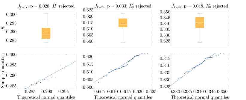

We illustrate the use of these plots in Fig. 12. In the top two rows we exhibit the three example jobs that failed the Shapiro-Wilk test for normality. For , the corresponding box plot is (i) not symmetric and (ii) has a mean that deviates significantly from its median. The QQ plot also deviates from a diagonal line, especially for larger fidelities. As we move from to and then , the data appears increasingly more normal but still fails the Shapiro-Wilk test. The extent to which they fail the visual tests is best seen by considering a normal-looking example, which we can glean from the bottom two rows of plots, which were not rejected by either hypothesis test.
For the data shown, is the closest data set to normal. Here, for Shapiro-Wilk, the box plot is symmetric, the mean/median agree, and the QQ plot data hardly deviates from the diagonal. Given this almost ideally normal data set, it is easier to see why the other data sets fail to appear as normal. For example, even those that pass hypothesis tests exhibit some non-normal features. But among those rejected, we see deviations from the diagonal line, skewness (a lack of symmetry in the box plot), and a discrepancy between the mean and the media.
Since most jobs (64/67) have data that passes hypothesis and visual normality tests, we conclude that Assumption Assumption 1 is reasonable.
Assumption 2.
Any demonstration within a fixed job is representative of any other identical demonstration within the same job. Hence, it is not necessary to repeat an identical demonstration within a fixed job. In other words, where is obtained by bootstrapping as in Section C.1 is a sufficient summary of the estimates and in .
Result 2.
Assumption Assumption 2 is justifying by a simple direct comparison of mean fidelity and standard deviation estimates. In particular, we compare (i) directly computing the sample mean and sample standard deviation and assuming normality, (ii) bootstrapping over the fidelities in , and (iii) bootstrapping over demonstration output counts used to compute . For all jobs (i.e., , the three methods are consistent with each other since the error bars have significant overlap in all cases. See Fig. 13.
The basic idea is that all three methods are consistent with each other. By consistency, we mean the intuitive notion that the error bars have significant overlap with each other. Further rigor, in this case, is not necessary due to the degree of matching with respect to job-to-job fluctuations we discuss below. This consistency is significant because the final method shown in Fig. 13 bootstraps only over the counts used to compute . Hence, it is sufficient to run an demonstration only once within a single job and use the results as being representative of repeating the identical demonstration, thereby showing the claimed result.

We next detail the methods leading to the three summaries in Fig. 13. The first is to summarize by the sample mean and sample standard deviation, where and By Result Result 1, it is appropriate to then characterize the sample with the first two moments — hence the name “assume normal.” The second and third methods, called “bootstrap ” and “bootstrap ”, both utilize the bootstrapping procedure discussed in Section C.1. The difference is in what is treated as the samples. In the case, we bootstrap over the values using , -sized samples. From these estimates of , we can estimate . We can then estimate the sample standard deviation It is important to note that here has the meaning of the standard deviation of our estimate of the mean. As , , so is not an estimate of as in some parametric distribution . To match the same meaning as the “assume normal” estimate, we report as the “bootstrap ” estimate. In the case, we bootstrap over the counts used to compute in exactly the same way as discussed in Section C.1. Hence, this method does not utilize the demonstrations for , and the sample standard deviation is an estimate of and is consistent with “assume normal.”
Assumption 3.
Given that can be modeled as samples from , data in a different job for but in the same calibration cycle can also be modeled as samples from .
Result 3.
Assumption Assumption 3 is not supported by the data we have already seen in Figs. 11,12, and 13. It is worth reiterating that this assumption does not hold even when the calibration is fixed or even when the jobs are contiguous.
In Fig. 11, we see box plots scattered wildly with median fidelities ranging from to and whose ranges do not overlap. Put more precisely, recall that when “assuming normality” as in Fig. 13, we can simplify each job’s results to a single estimate . Once we have done that, we find and and yet , so it is not possible for all the data to be consistent as described in Assumption Assumption 3. This discrepancy is not resolved when considering jobs that are time-proximate or contiguous, as we have discussed before. To see this, note that all jobs were taken within a ten-hour window for a fixed calibration: the first nine jobs were taken within the first hour, the first three of which within the first ten minutes. Despite this, there are large variations that violate Assumption Assumption 3 even within the first three jobs.
This result is the first major departure from expectations; it tells us that an demonstration must be repeated many times across different jobs to estimate the variance in performance from run to run. One consequence is that if we test the preservation of in job 1 and in job 2, it is not reliable to compare the fidelities and and draw conclusions about the results of a generic demonstration testing both and . Alternatively, if we test the efficacy of two sequences and given the same state but where the data is taken from different jobs, this is not a reliable indicator of their individual relative performance either. Instead, many demonstrations must be taken where the variance can be estimated, or direct comparisons should only be made within a fixed job and then repeated to check for the stability of the result.
The next two assumptions and results address to what extent data taken across different jobs, or even calibrations, can be modeled as being normally distributed.
Assumption 4.
It is appropriate to model for some fixed calibration cycle provided all jobs are in . In other words, demonstrations taken from different jobs can be viewed as sampled from a fixed normal distribution.
Result 4.
This assumption is justified since it is not rejected by the Jaque-Bera and Shapiro-Wilk hypothesis tests and is supported by visual indicators (box plot, QQ plot, and error bar comparison plot).
Let be the set of the first empirical fidelity from each job. Given this data set, neither the Jaque-Bera nor the Shaprio-Wilk test support rejecting the hypothesis that . More precisely, the -values are and , respectively, so with 95% confidence, we cannot reject the hypothesis.
In addition, we show the standard visual tests — box plot and QQ plot — in Fig. 14 alongside the error bar comparison plot similar to Fig. 13. The standard visual tests also support assuming normality since the box plot is symmetric, has a mean and median that almost agree, and the QQ plot data lies mostly along the diagonal. However, perhaps the most important evidence is the error bar comparison (bottom panel). By “assume normal”, we compute the sample mean () and standard deviation of of as the estimates of and . We find and . Hence, we would report as the average fidelity value across the fixed calibration. When instead bootstrapping the samples of , we again find , which remarkably has symmetric error bars.
Hence, in all, it is reasonable to model the fidelity samples from different jobs as samples of a fixed normal distribution within a fixed calibration cycle. Note that we were careful not to try and model the entire data set as normal; instead, we held the number of samples from each job constant. Had we modeled the entirety of the data set, the Jaque-Bera and Shaprio-Wilk tests would reject normality. This is because some samples are unfairly given more weight, which is no longer normal.141414By taking a different number of samples, it is as if we roll a die but write down the answer a random number of times. This sampling strategy takes longer to converge to the expected result.


Assumption 5.
Let be empirical fidelity samples similar to from before but not necessarily sampled from a fixed calibration. Then even across different calibrations.
Result 5.
This assumption is justified for the free evolution (Free) data but is violated for some DD sequences such as KDD. Nevertheless, for average point-wise fidelity estimates of the form , the difference between assuming normality or bootstrapping is negligible.
Here, we will need to consider a different data set for the first time in this series of assumptions and tests. Instead of considering data from a fixed time , we consider fidelity decay data as in Figs. 7 and 8. Namely, we consider the preservation of and under Free and KDD as a function of time. In each case, we consider the fidelity at twelve roughly equidistant time steps for . Here, is a placeholder for the sequence (Free or KDD), for the calibration at which the fidelity was sampled, and for the state. We test the normality for each set of fixed , which amounts to a set such as in Assumption Assumption 4.
We begin by applying both the Jarque-Bera and Shaprio-Wilk hypothesis tests. We tabulate the cases where the hypothesis of normality fails with 95% confidence in Table 4. According to these tests, we can confidently claim that the set of KDD fidelity decay curves for does not obey all the properties we would expect for samples of a series of normal distributions. Namely, the times for do not have the right order statistics since they fail the Shapiro-Wilk test. This seems reasonable given Fig. 7, in which the KDD data appears to bi-modal for the middle times.
| rejected by JB | rejected by SW | ||
|---|---|---|---|
| Free | {6} | {6} | |
| Free | {2} | {2} | |
| KDD | {} | {3,4,5,6,7,8,9} | |
| KDD | {6} | {6,7,8} |
We can also consider box plots for the data which support the claims made in Table 4. As an example, in Fig. 15 we show the box plot for (Free, ), which agrees with normality at each time point, and (KDD, , which fails to appear normal at most time points.


Despite not passing the tests for normality, we can still formally pretend that the data is normal and compute the sample mean and variance as estimates of and . When we do this and compare the result to bootstrapping the mean and rescaling the confidence interval, the results are almost identical for both sets of data, as we can see in Fig. 16. By rescaling the confidence interval (CI), we mean we compute the 95% CI of the mean estimate by bootstrapping, , and report where is the number of calibration cycles (i.e., the number of fidelities) we bootstrap over. The rescaling is done to obtain an estimate of the spread of the underlying distribution and not of the sample mean. In other words, we observe that averaging via the bootstrap or by the simple sample mean and standard deviation agree even for pathological data of the form we obtain for KDD.
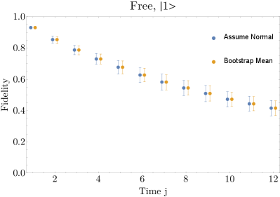

This observation seems to suggest that we can compare DD sequences by first averaging fidelities across calibrations. This would be in line with preview work such as Refs. [41, 98] that did not report on the subtleties of job-to-job variation. As outlined in the main text and implied by the analysis presented in this appendix, we choose not to do this; the next section clarifies why and what we do instead.
C.7 Effect of job-to-job fluctuations
Let be a fidelity sample for state and calibration for some fixed time and sequence. We saw in Result Result 5 that assuming is not formally justified for all sequences and states. In particular, the state decay for KDD does not pass hypothesis tests for normality at intermediate times. Nevertheless, if we are only concerned with the average fidelity of a fixed state across calibrations,
| (61) |
assuming normality or bootstrapping leads to consistent predictions. But related work—such as Refs. [41, 98]—was concerned with the average fidelity across states,
| (62) |
for some set of states and fixed calibration . If and IID, then where and Thus, we would expect the state-average fidelity to be consistent from job to job. In practice, however, this does not happen. For example, the Pauli averaged-fidelity (i.e., choosing ) for different calibrations for the KDD sequence at time is given in Fig. 17.

The inconsistency of the average state fidelity as exhibited in Fig. 17 has several consequences. First, data from a single calibration is generally not enough to characterize typical behavior. For example, if we only sampled a single calibration and happened to sample , we would be left with the wrong impression of KDD’s performance. Second, data from a single calibration is also generally not representative of average behavior. Indeed, the red dot in the middle corresponds to the average over the calibration averages, and no single calibration has a mean consistent with this average. Finally, averaging over states sampled in different jobs can lead to misleading results. For example, suppose we queued up several runs of in calibration , of in , etc…. Then, according to the average fidelities in Fig. 17, it is likely that a run in would have substantially higher fidelity than a run in . Yet, if we compared to within the same calibration, they would have roughly the same fidelity.
To clarify this averaging subtlety, we present the raw data for each state as a box plot in Fig. 18. The variation arises from the fidelity fluctuations of each state across calibrations. Interestingly, the polar states, and , give surprisingly consistent results, while the remaining equatorial states have large variations in performance. This suggests that in some calibrations, the equatorial states were adversely affected, while the polar states were mostly unaffected. By checking the data calibration-by-calibration, we find this to indeed be true. Namely, the equatorial states collectively have a similar performance that is worse in some calibrations and better in others. This could happen, e.g., if, in some calibrations, dropped while stayed roughly the same. Thus, to have a direct comparison of state performance, it is imperative to confine the comparison to within a single job. The same can be said about comparing the fidelities of a fixed state generated at different times. Without confining comparisons to a single job, it is unknown if the difference in fidelities is due to drift or other causes.

On the other hand, it is not possible to test all DD sequences, states, and decay times within a short enough window to avoid significant drift. Even if it were, fair-queuing enforces a maximum number of circuits per job, so this sets a hard cut-off on what can be compared reliably in a time-proximate way. As a compromise between time-proximate comparisons and the hard circuits-per-job limit, we collected data as described in Section III. Namely, within a single job, we collect the fidelity decay curves for the six Pauli states. Each curve consists of time points. In total, this takes up circuits, and we pad this with an additional set of two measurement error mitigation circuits. In this sense, we guarantee that the fidelities for different states and times can be compared reliably within this data set, i.e., they are not different due to drift. We then repeat this demonstration over different calibration cycles to obtain an estimate of fidelity differences due to drift. By reporting the median across this data set, we provide an estimate of typical performance — the performance estimate of a hypothetical next demonstration. We emphasize that the typical performance is different from the average performance.
To further support this point, we have included average fidelities (with bootstrapped 95% confidence intervals) superimposed on the box plots in Fig. 18. For all data sets, the mean and median do not agree. For the polar states ( and , the difference is slight, and their respective median performance is included in the error bar of the mean. We remark that averages and medians generally agree as they do here for the best performing DD sequences (see Fig. 3). The mean is heavily biased downward for the remaining equatorial states, and the confidence intervals do not include the mean. Once averaging over the entire data set, the discrepancy is even worse. Here, the mean falls on top of the 25% quantile, and the top of the confidence interval differs from the median by a significant amount. Hence, an average method is inappropriate for DD sequences whose performance is highly sensitive to drift effects, and a median method is more appropriate. Again, we remark that this should not affect the top performing sequences shown in Fig. 3, but it gives us a consistent way to sift through all the sequences at once to even get to a top ranking in the first place.
To summarize, we have shown that averaging fidelities over states is a delicate issue that depends on how the data is averaged. When averaging within a fixed job, the results appear reasonable and simple averaging of the fidelities over states gives an average state fidelity that behaves as expected. When comparing state data across different jobs, a straightforward average can be biased due to a particularly bad calibration, resulting in an average sensitive to drift. A non-parametric comparison in which fidelities are assessed via a box plot, on the other hand, does not suffer from this issue. When confined to a fixed job, the median over states gives a measure of typical performance over the set of states. When fidelities are collected over both states and calibrations, the median is still a measure of typical performance, but now over both states and calibrations. Hence, a measure of typical performance is more robust than an average performance metric when considering drift. In practice, typical performance is more relevant for any given fixed demonstration. These facts, alongside the practical difficulties of averaging and fitting, are why we opted for the fit-then-average (FtA) approach.
C.8 Summary of fitting fidelity
The standard approach to comparing DD sequences is to generate average fidelity decay curves, fit them, and report a summary statistic like a decay constant. For this reason, we call this an “average-then-fit” (AtF) approach. In Ref. [41], for example, the authors generated fidelity decay curves for roughly 40 equally spaced times and states ( Haar-random and six Pauli eigenstates). For each time, they computed a state-average fidelity constituting a single average fidelity decay curve. They then fit this curve to a modified exponential decay [Eq. 59] and reported the decay constant for XY4 compared to Free evolution. This was sufficient to show that, on average, applying XY4 was better than free evolution.
In this work, we aim to go beyond this approach and identify any pitfalls. To do so, we set out to first compare a large collection of DD sequences and not just XY4 and Free. Second, we are interested in whether XY4 retains universality for superconducting devices (see Section II.4). This question requires us to know precisely whether, e.g., or is better protected under XY4. This led us to two methodological observations. (i) Using a standard fit such as Eq. 59 to individual state decay curves results in several problems: it does not always work in practice, leading to an ambiguous interpretation of the decay constant, and it requires a complicated fitting procedure. (ii) The fidelity of a given state protected with DD for a fixed time is unstable from job to job due to device drift. This means one must be careful when comparing fidelities not collected within the same job.
We resolved both issues by (i) focusing on typical performance instead of average and (ii) using a “fit-than-average” (FtA) approach where we interpolate with time-averaging (ITA). Along the way, the insistence on not first averaging results in the identification of significant and unexpected asymmetries in performance between states (see Appendix B and especially Fig. 6), which led to better DD sequence design. Ultimately, more than the issues with fitting leading to ambiguous/inconsistent results described in Section C.5, it is the core idea of comparing data within a given job that led to our eventual choice of analysis method.
C.9 Details of fitting using Mathematica
C.9.1 Standard fit to exponential details
At a high level, we fit the fidelity decay curves (see Fig. 7 for example curves and Fig. 8 for example curves with fits) to Eq. 59 using Mathematica’s NonlinearModelFit (NLM) [99, 100] which performs weighted least-squares regression. In more detail, NLM finds the parameters which minimize the weighted sum of squares,
| (63) |
with the assumption that
| (64) |
for some unknown parameters and . Given a good model and fitting procedure, the NLM procedure finds , and [101]. Furthermore, NLM computes the covariance matrix, , between the estimated parameters,
| (65a) | ||||
| (65b) | ||||
| (65c) | ||||
where is the integrated fidelity [Eq. 58] and this particular form of and results from setting the Weights and VarianceEstimatorFunction NLM settings appropriately for experimental data.151515The choice of weights is exactly as stated in Eq. 65c, but the variance estimator setting is more subtle. We set the variance estimator to the constant 1, which prevents the covariance matrix from being rescaled by a variance estimate of in Eq. 64. We do this since we do not need to estimate –we already did this by performing our demonstration, and the weight matrix reflects this knowledge. These settings are discussed in Mathematica’s Fit Models with Measurement Errors tutorial. As usual, we compute the parameter standard errors (aka the standard deviations of the statistics) from the covariance matrix as,
| (66) |
From this, we can estimate the parameter 95% confidence intervals by calculating a t-score. To do this, we first find the number of degrees of freedom we have, . The t-score is then the such that
| (67) |
In the end, we report our best-fit parameters with 95% confidence using
| (68) |
with an exactly analogous formula for and (i.e., same throughout).161616We spell out the details for completeness, but the estimate for can be immediately returned from NLM using the “ParameterConfidenceIntervals” option without needing to compute the covariance matrix directly at all.
C.9.2 Consistency checks and selecting appropriate fitting options
The previous section outlined the general methodology and output of Mathematica’s NonlinearModelFit function. One detail we glossed over is the method by which NonlinearModelFit minimizes the weighted sum of squares, . By default, is minimized using the LevenbergMarquardt method — a particular implementation of the Gauss–Newton algorithm. Many of the details and optimization settings are outlined in Mathematica’s “Unconstrained Optimization: Methods for Local Minimization” documentation. An important feature of this method is that it is a local search method, and hence, the quality of the fit depends on the particular input settings and randomness in each run. Coupled with the fact that , , and of Eq. 59 are not independent parameters, it is important in practice to try many different settings to obtain a good fit. A full enumeration of all settings we attempted can be found in the fittingFreeData.nb Mathematica notebook contained in our code repository [93]. For example, we consider fits for which we reduce the number of parameters (e.g., setting ) or where is either seeded or unseeded.
Upon trying many possible fits, we then need an objective way to compare their relative quality. To do so from a fit obtained using NonlinearModelFit, one can query its associated (corrected) Akaike information criterion (AICc) [102] via Mathematica’s Fit["AICc"]. The AIC estimates the relative quality of each model in a collection of models for a given data set. In our case, the sample size is relatively small: points for each fit. To remedy this, we employ the AICc, which corrects the tendency of AIC to favor overfitting for small sample sizes. See Ref. [102] for a summary of the formulas for AIC and AICc. A more detailed introduction and derivations of the formulas can be found in Ref. [103, pp. 51-74].
The lower the AICc, the better the model is relative to others. However, we must also ensure that the final fit satisfies consistency conditions. Namely, a fit is considered unreasonable if it (a) predicts a fidelity less than zero or greater than one, (b) predicts a parameter whose error is larger than the value itself, or (c) violates the Nyquist-Shannon sampling theorem [104], i.e., has frequency larger than the sample rate of the data itself. I.e., in Eq. 59 must satisfy where is the spacing between data points in our fidelity decay curves. After fitting, we reject fits which violate properties (a) and (b) and correct those that violate (c). We next illustrate what this post-selection or correction looks like for our data.
First, we perform many fits without regard to whether (a)-(c) are satisfied since enforcing constraints makes the nonlinear fit results unstable, and moreover, the constraints are not always enforced even when specified inside NonlinearModelFit. We then post-select the fits that respect (a) and (b), and among these, we select the fit with the lowest AICc. If no fit respecting (a) and (b) is found, we drop that data set. Finally, we rescale the frequency via This procedure — along with the fits along the way — is summarized in Fig. 19. Note that we are forced to post-select fits that are well modeled by Eq. 59 in order to report a reasonable value of for the given data. For this reason, the fitting procedure thus described is biased toward data that is appropriately modeled by Eq. 59.


C.9.3 Time-averaged fidelity approach
We construct a polynomial interpolation of the fidelity decay data using Mathematica’s Interpolation function [99, 105]. Then we integrate over the interpolation to compute a time-averaged fidelity according to Eq. 58. By default, the Interpolation uses a third-order Hermite method [106] which we found to be sufficient to model our data adequately. For example, the curves in Fig. 7 consist of Hermite interpolations of the triangular raw data, which appears reasonable. To compute Eq. 58 from the interpolation, we used Mathematica’s NIntegrate.


For a sense of stability, we also tried the popular cubic spline interpolation method [107], but this does not affect our results outside of the interpolation error bound itself. For example, consider the complicated interpolation necessary for KDD using the Hermite or cubic spline methods in Fig. 20. Hence, either interpolation is equally valid when using the time-averaged fidelity metric.
We remark that polynomial interpolation is much easier to do than fitting to a model such as Eq. 59 since we need not (i) select reasonable fitting equations, (ii) fit them using nonlinear least squares regression, (iii) post-select fits with satisfy consistency conditions and low AICc. Additionally, the predictions are less susceptible to ambiguities as described in Section C.5. Finally, we are not forced to discard any data sets which fail the post-selection criteria, so we do not bias the final summary results in any particular way.
Appendix D Toggling frame
We assume that without any external control, the system and bath evolve under the time-independent noise Hamiltonian . A DD pulse sequence is realized via a time-dependent control Hamiltonian acting only on the system so that the system and bath evolve according to (refer to Section II.1 for definitions of the various Hamiltonian terms).
For understanding the effects of the control Hamiltonian, it is convenient to use the interaction picture defined by , also known as the toggling frame [108, 21, 31, 109, 34]. The toggling-frame density operator is related to the Schrödinger-picture density operator by
| (69) |
where is the evolution operator generated by the full Hamiltonian . Therefore the toggling-frame state evolves according to
| (70) |
where the toggling-frame time evolution operator
| (71) |
is generated by the toggling-frame Hamiltonian
| (72) |
Since acts nontrivially only on the system, can be written as
| (73) |
where is the toggling-frame version of . Because the operator norm is unitarily-invariant, we have and .
Throughout, we consider cyclic DD, where returns to the identity (up to a possible irrelevant overall phase) at the end of a cycle taking time :
| (74) |
Therefore, at the end of the cycle, the toggling-frame and Schrödinger-picture states coincide.
Appendix E Results of all Pauli demonstrations
In Fig. 3, we summarized the results of the Pauli demonstration for the top sequences on each device and the baseline of CPMG, XY4, and free evolution. This appendix presents the data for all tested sequences. In particular, we split the data for each device into a grid of plots shown in Figs. 21-23, separating by family as in Table 1 when possible. For convenience, CPMG, XY4, and Free are still included in all plots along with colored reference lines matching the convention in Fig. 3. The purple reference line denotes the best sequence in the given family plot excluding the baseline sequences placed at the end. For example, in Fig. 21(b) is the best RGA sequence even though it does not outperform XY4; it is marked with a purple reference line.
We plot the same families for each device in a grid, labeled (a)-(i). In each caption, we make a few general comments on DD performance overall and then comment on observations specific to each sequence family. Recall that a specific definition of each sequence is given in Appendix A, and a summary of their properties along with references in Table 1. To avoid excessive repetition in each caption, we first provide a brief description of each of the cases (a)-(i) shown in Fig. 21-23:
-
(a)
This “family” serves as a catch-all for the basic sequences Hahn [55], CPMG [57, 72], and XY4 [56], along with sequences born from their modifications. Namely, we also plot the Eulerian super-cycle versions [80, 73] (denoted by S), KDD [48, 75] which is a composite pulse XY4, and [50, 88] which is a recursive embedding of XY4.
-
(b)
The robust genetic algorithm (RGA) family [74].
-
(c)
The universally robust (UR) family [54].
-
(d)
The Uhhrig dynamical decoupling (UDD) family using pulses, UDDx [51].
-
(e–i)
The quadratic dynamical decoupling (QDD) family with same inner and outer order, , with fixed outer order 1, with fixed outer order 2, with fixed outer order 3, , and with fixed outer order 4, , respectively [52].
For each family, we expect the empirical hierarchy of sequence performance to be a complicated function of device-specific properties. Specifically, actual performance is a competition between (i) error cancellation order, (ii) number of free evolution periods, and (iii) systematic pulse errors due to finite width and miscalibrations, among other factors discussed in Section II. For each family, we summarize our expectations regarding these factors
-
(a)
For ideal pulses, we expect . With a finite bandwidth constraint, we expect to only hold up until some optimal concatenation level after which performance saturates. Using finite width pulses with systematic errors, we expect (and similarly for other S sequences) and provided the additional robustness is helpful. I.e., if the pulses are extremely well calibrated and errors are dominated by latent bath-induced errors, then we should instead see .
-
(b)
The expected performance hierarchy for RGA is rather complicated, as indicated by the labeling, and is best summarized in depth using Table II of Ref. [74]. A quick summary is that if we have strong pulses dominated by miscalibration errors (), then we expect and to do well. In the opposite limit, we expect to do well. The increasing number indicates the number of pulses, and as this increases, the decoupling order increases, and the same competition between order-cancellation and free evolution periods as in also applies.
-
(c)
The sequence provides suppression of flip angle errors at the expense of using free evolution periods. The relationship of to decoupling is not well established in Ref. [54], but by construction seems to be for all . Thus our expectation is that improves with increasing until performance saturates and the contribution dominates the contribution. To see this, note that for a fixed time, the number of free evolution periods will be roughly the same regardless of .
-
(d)
Ideally, for a fixed demonstration duration , the performance of should scale as , and hence improves monotonically with increasing . In practice, this performance should saturate once the finite-pulse width error is the dominant noise contribution.
-
(e–i)
An extensive numerical study of performance is discussed in Ref. [66] with corresponding rigorous proofs in Ref. [68]. For ideal pules, the decoupling order is expected to be at least where is the total evolution time of implementing a single repetition. Since we are instead interested in a fixed total time consisting of multiple sequence repetitions with a minimal pulse interval, the interplay of competing factors is quite complicated. Further, we are forced to apply rotations about , , and to implement when is odd, but as noted in Appendix B, is virtual without OpenPulse. In summary, the naive theoretical expectation is that should improve with increasing , eventually saturating for the same reasons as . However, we expect the fixed and virtual- set-up to complicate the actual results.

(a) Results are not consistent with ideal-pulse theory but are sensible when considering realistic competing factors. First, S-Hahn Hahn and S-CPMG CPMG are consistent with the large pulse widths on ibmq_armonk, for which ns. That XY4 works very well is also consistent with its expected approximate universality given that on ibmq_armonk. Given that XY4 already performs well, it is not surprising that its robust versions, S-XY4 and KDD, do worse. In particular, they have little room for improvement but also add extra free evolution periods that accumulate additional error. Finally, is roughly flat for all tested, which is consistent with an expected saturation that happens to occur at .
(b) The performance of RGA does not match theoretical expectations. To see this, note that is itself a four-pulse sequence with error scaling which is the same as XY4. Hence, it should perform comparably to XY4, but it does significantly worse. Furthermore, it is also unexpected that the best RGA sequences are 8a, 64a, and 64c. Indeed, 8a and 64a are expected to work best in a flip-angle error dominated regime, but in this regime, 64c has a scaling of , so it is not expected to do well.
(c) The sequence performance is consistent with theory. First note that . Thus, we expect for to improve upon or saturate at the performance of XY4, and the latter is what happens.
(d) The sequence performance is consistent with theory. In particular, we expect (and observe) a consistent increase in performance with increasing until performance saturates.
(e-i) The results in part match theoretical expectations, since they exhibit a strong even-odd effect, as predicted in Refs. [66, 68, 71]. Nevertheless, the optimal choice of and has to be fine-tuned for ibmq_armonk. We note that five out of ten of the top ten sequences on ibmq_armonk are from the QDD family.
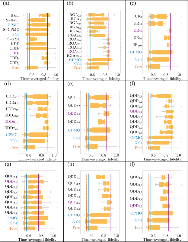
(a) Results are not fully consistent with ideal-pulse theory. For example, it is unexpected that Hahn CPMG and that Hahn S-Hahn while at the same time S-XY4 XY4. Nevertheless, some trends are expected such as and then saturating.
(b) Results are somewhat consistent with ideal-pulse theory. First of all, in performance, which is sensible. The first large improvement comes from and then from numbers and greater. This trend is similar to increasing, which is expected since larger RGA sequences are also recursively defined (e.g., is a recursive embedding of into itself). However, it is again unexpected that both ‘a’ and ‘c’ sequences should work well at the same time. For example, theoretically means that ibmq_bogota has negligible flip angle error. In such a regime, the decoupling order of is the same as since they are designed to cancel flip-angle errors. But, we find that in practice.
(c) The results are mostly consistent with theory. First, is an improvement over XY4, and though does increase with larger , it is not simply monotonic as one would expect in theory. Instead, we find a more general trend with an empirical optimum at .
(d) The results are mostly consistent with expectations. Again, performance mostly increases with increasing , but the increase is not fully monotonic.
(e-i) The results are fairly consistent with theory. In (e), performance of increases with until . The degradation for is consistent with expectations in the bandwidth-limited setting [69]. In (f - i) the results are again fairly expected: aside from parity effects (odd/even ), for , we expect monotonic improvement with increasing until , after which performance should saturate or even slightly improve; this is the general empirical trend.

(a) Results are not fully consistent with ideal-pulse theory. For example, it is unexpected that Hahn CPMG and that Hahn S-Hahn while at the same time S-XY4 XY4. Nevertheless, some trends are expected, such as and then saturating.
(b) Results are somewhat consistent with the theory. First of all, is sensible and implies that we are in a flip-angle error dominated regime. However, we would then expect , which does not occur. Nevertheless, the recursively defined sequences (number and above) generally outperform their shorter counterparts, which is similar to as expected.
(c) The results are consistent with theory. First, is a large improvement over XY4, and from there . After this, the improvement plateaus.
(d) The performance of greatly differs from the theoretical expectation of monotonic improvement with . In fact, the behavior is so erratic that we suspect device calibration errors dominated the demonstration. Nevertheless, the performance of was excellent in this case.
(e-i) The results are fairly consistent with theory, and quite similar to Fig. 22. The same comments as made there apply here.
References
- Montanaro [2016] A. Montanaro, Quantum algorithms: An overview, NPJ Quantum Inf. 2, 15023 (2016).
- Preskill [2018] J. Preskill, Quantum Computing in the NISQ era and beyond, Quantum 2, 79 (2018).
- Daley et al. [2022] A. J. Daley, I. Bloch, C. Kokail, S. Flannigan, N. Pearson, M. Troyer, and P. Zoller, Practical quantum advantage in quantum simulation, Nature 607, 667 (2022).
- Campbell et al. [2017] E. T. Campbell, B. M. Terhal, and C. Vuillot, Roads towards fault-tolerant universal quantum computation, Nature 549, 172 EP (2017).
- Gottesman [2022] D. Gottesman, Opportunities and challenges in fault-tolerant quantum computation (2022), arXiv:2210.15844 [quant-ph] .
- Pudenz et al. [2014] K. L. Pudenz, T. Albash, and D. A. Lidar, Error-corrected quantum annealing with hundreds of qubits, Nat. Commun. 5, 3243 (2014).
- Devitt [2016] S. J. Devitt, Performing quantum computing experiments in the cloud, Physical Review A 94, 032329 (2016).
- Vinci et al. [2016] W. Vinci, T. Albash, and D. A. Lidar, Nested quantum annealing correction, npj Quant. Inf. 2, 16017 (2016).
- Wootton and Loss [2018] J. R. Wootton and D. Loss, Repetition code of 15 qubits, Physical Review A 97, 052313 (2018).
- Vuillot [2018] C. Vuillot, Is error detection helpful on ibm 5q chips ?, Quantum Inf. Comput. 18, 18, 0949 (2018).
- Roffe et al. [2018] J. Roffe, D. Headley, N. Chancellor, D. Horsman, and V. Kendon, Protecting quantum memories using coherent parity check codes, Quantum Science and Technology 3, 035010 (2018).
- Willsch et al. [2018] D. Willsch, M. Willsch, F. Jin, H. De Raedt, and K. Michielsen, Testing quantum fault tolerance on small systems, Physical Review A 98, 052348 (2018).
- Pearson et al. [2019] A. Pearson, A. Mishra, I. Hen, and D. A. Lidar, Analog errors in quantum annealing: doom and hope, npj Quantum Information 5, 107 (2019).
- Harper and Flammia [2019] R. Harper and S. T. Flammia, Fault-tolerant logical gates in the ibm quantum experience, Physical Review Letters 122, 080504 (2019).
- Ryan-Anderson et al. [2021] C. Ryan-Anderson, J. Bohnet, K. Lee, D. Gresh, A. Hankin, J. Gaebler, D. Francois, A. Chernoguzov, D. Lucchetti, N. Brown, et al., Realization of real-time fault-tolerant quantum error correction, Physical Review X 11, 041058 (2021).
- Chen et al. [2021] Z. Chen, K. J. Satzinger, J. Atalaya, A. N. Korotkov, A. Dunsworth, D. Sank, C. Quintana, M. McEwen, R. Barends, P. V. Klimov, S. Hong, C. Jones, A. Petukhov, D. Kafri, S. Demura, B. Burkett, C. Gidney, A. G. Fowler, A. Paler, H. Putterman, I. Aleiner, F. Arute, K. Arya, R. Babbush, J. C. Bardin, A. Bengtsson, A. Bourassa, M. Broughton, B. B. Buckley, D. A. Buell, N. Bushnell, B. Chiaro, R. Collins, W. Courtney, A. R. Derk, D. Eppens, C. Erickson, E. Farhi, B. Foxen, M. Giustina, A. Greene, J. A. Gross, M. P. Harrigan, S. D. Harrington, J. Hilton, A. Ho, T. Huang, W. J. Huggins, L. B. Ioffe, S. V. Isakov, E. Jeffrey, Z. Jiang, K. Kechedzhi, S. Kim, A. Kitaev, F. Kostritsa, D. Landhuis, P. Laptev, E. Lucero, O. Martin, J. R. McClean, T. McCourt, X. Mi, K. C. Miao, M. Mohseni, S. Montazeri, W. Mruczkiewicz, J. Mutus, O. Naaman, M. Neeley, C. Neill, M. Newman, M. Y. Niu, T. E. O’Brien, A. Opremcak, E. Ostby, B. Pató, N. Redd, P. Roushan, N. C. Rubin, V. Shvarts, D. Strain, M. Szalay, M. D. Trevithick, B. Villalonga, T. White, Z. J. Yao, P. Yeh, J. Yoo, A. Zalcman, H. Neven, S. Boixo, V. Smelyanskiy, Y. Chen, A. Megrant, J. Kelly, and G. Q. AI, Exponential suppression of bit or phase errors with cyclic error correction, Nature 595, 383 (2021).
- Viola and Lloyd [1998] L. Viola and S. Lloyd, Dynamical suppression of decoherence in two-state quantum systems, Phys. Rev. A 58, 2733 (1998).
- Zanardi [1999a] P. Zanardi, Symmetrizing evolutions, Physics Letters A 258, 77 (1999a).
- Vitali and Tombesi [1999] D. Vitali and P. Tombesi, Using parity kicks for decoherence control, Physical Review A 59, 4178 (1999).
- Duan and Guo [1999] L.-M. Duan and G.-C. Guo, Suppressing environmental noise in quantum computation through pulse control, Physics Letters A 261, 139 (1999).
- Viola et al. [1999a] L. Viola, E. Knill, and S. Lloyd, Dynamical decoupling of open quantum systems, Physical Review Letters 82, 2417 (1999a).
- Biercuk et al. [2009a] M. J. Biercuk, H. Uys, A. P. VanDevender, N. Shiga, W. M. Itano, and J. J. Bollinger, Optimized dynamical decoupling in a model quantum memory, Nature 458, 996 (2009a).
- Biercuk et al. [2009b] M. J. Biercuk, H. Uys, A. P. VanDevender, N. Shiga, W. M. Itano, and J. J. Bollinger, Experimental uhrig dynamical decoupling using trapped ions, Phys. Rev. A 79, 062324 (2009b).
- Damodarakurup et al. [2009] S. Damodarakurup, M. Lucamarini, G. D. Giuseppe, D. Vitali, and P. Tombesi, Experimental inhibition of decoherence on flying qubits via “bang-bang” control, Phys. Rev. Lett. 103, 040502 (2009).
- Du et al. [2009] J. Du, X. Rong, N. Zhao, Y. Wang, J. Yang, and R. B. Liu, Preserving electron spin coherence in solids by optimal dynamical decoupling, Nature 461, 1265 (2009).
- Jenista et al. [2009] E. R. Jenista, A. M. Stokes, R. T. Branca, and W. S. Warren, Optimized, unequal pulse spacing in multiple echo sequences improves refocusing in magnetic resonance, J. Chem. Phys. 131, 204510 (2009).
- Álvarez et al. [2010] G. A. Álvarez, A. Ajoy, X. Peng, and D. Suter, Performance comparison of dynamical decoupling sequences for a qubit in a rapidly fluctuating spin bath, Phys. Rev. A 82, 042306 (2010).
- Peng et al. [2011] X. Peng, D. Suter, and D. A. Lidar, High fidelity quantum memory via dynamical decoupling: theory and experiment, Journal of Physics B: Atomic, Molecular and Optical Physics 44, 154003 (2011).
- Sagi et al. [2010] Y. Sagi, I. Almog, and N. Davidson, Suppression of collisional decoherence in optically trapped atomic ensemble by bang-bang dynamical decoupling, in CLEO/QELS: 2010 Laser Science to Photonic Applications (2010) pp. 1–2.
- Wang et al. [2012] Z.-H. Wang, G. de Lange, D. Ristè, R. Hanson, and V. V. Dobrovitski, Comparison of dynamical decoupling protocols for a nitrogen-vacancy center in diamond, Physical Review B 85, 155204 (2012).
- Viola et al. [1999b] L. Viola, S. Lloyd, and E. Knill, Universal control of decoupled quantum systems, Phys. Rev. Lett. 83, 4888 (1999b).
- Viola [2002] L. Viola, Quantum control via encoded dynamical decoupling, Phys. Rev. A 66, 012307 (2002).
- Khodjasteh and Lidar [2002] K. Khodjasteh and D. A. Lidar, Universal fault-tolerant quantum computation in the presence of spontaneous emission and collective dephasing, Physical Review Letters 89, 197904 (2002).
- Viola and Knill [2005] L. Viola and E. Knill, Random decoupling schemes for quantum dynamical control and error suppression, Phys. Rev. Lett. 94, 060502 (2005).
- Khodjasteh and Lidar [2008] K. Khodjasteh and D. A. Lidar, Rigorous bounds on the performance of a hybrid dynamical-decoupling quantum-computing scheme, Physical Review A 78, 012355 (2008).
- Lidar [2008] D. A. Lidar, Towards fault tolerant adiabatic quantum computation, Phys. Rev. Lett. 100, 160506 (2008).
- West et al. [2010a] J. R. West, D. A. Lidar, B. H. Fong, and M. F. Gyure, High fidelity quantum gates via dynamical decoupling, Phys. Rev. Lett. 105, 230503 (2010a).
- van der Sar et al. [2012] T. van der Sar, Z. H. Wang, M. S. Blok, H. Bernien, T. H. Taminiau, D. M. Toyli, D. A. Lidar, D. D. Awschalom, R. Hanson, and V. V. Dobrovitski, Decoherence-protected quantum gates for a hybrid solid-state spin register, Nature 484, 82 (2012).
- Ng et al. [2011] H. K. Ng, D. A. Lidar, and J. Preskill, Combining dynamical decoupling with fault-tolerant quantum computation, Phys. Rev. A 84, 012305 (2011).
- Paz-Silva and Lidar [2013] G. A. Paz-Silva and D. A. Lidar, Optimally combining dynamical decoupling and quantum error correction, Sci. Rep. 3 (2013).
- Pokharel et al. [2018] B. Pokharel, N. Anand, B. Fortman, and D. A. Lidar, Demonstration of fidelity improvement using dynamical decoupling with superconducting qubits, Physical Review Letters 121, 220502 (2018).
- Souza [2021] A. M. Souza, Process tomography of robust dynamical decoupling with superconducting qubits, Quantum Information Processing 20, 237 (2021).
- Jurcevic et al. [2021] P. Jurcevic, A. Javadi-Abhari, L. S. Bishop, I. Lauer, D. F. Bogorin, M. Brink, L. Capelluto, O. Günlük, T. Itoko, N. Kanazawa, A. Kandala, G. A. Keefe, K. Krsulich, W. Landers, E. P. Lewandowski, D. T. McClure, G. Nannicini, A. Narasgond, H. M. Nayfeh, E. Pritchett, M. B. Rothwell, S. Srinivasan, N. Sundaresan, C. Wang, K. X. Wei, C. J. Wood, J.-B. Yau, E. J. Zhang, O. E. Dial, J. M. Chow, and J. M. Gambetta, Demonstration of quantum volume 64 on a superconducting quantum computing system, Quantum Sci. Technol. 6, 025020 (2021).
- Tripathi et al. [2022] V. Tripathi, H. Chen, M. Khezri, K.-W. Yip, E. M. Levenson-Falk, and D. A. Lidar, Suppression of crosstalk in superconducting qubits using dynamical decoupling, Physical Review Applied 18, 024068 (2022).
- Pokharel and Lidar [2022a] B. Pokharel and D. Lidar, Better-than-classical Grover search via quantum error detection and suppression (2022a), arXiv:2211.04543 [quant-ph] .
- Zhou et al. [2022] Z. Zhou, R. Sitler, Y. Oda, K. Schultz, and G. Quiroz, Quantum crosstalk robust quantum control (2022), 2208.05978 [quant-ph] .
- Pokharel and Lidar [2022b] B. Pokharel and D. A. Lidar, Demonstration of algorithmic quantum speedup (2022b), arXiv:2207.07647 [quant-ph] .
- Souza et al. [2012] A. M. Souza, G. A. Álvarez, and D. Suter, Robust dynamical decoupling, Philosophical Transactions of the Royal Society A: Mathematical, Physical and Engineering Sciences 370, 4748 (2012).
- Capelluto and Alexander [2021] L. Capelluto and T. Alexander, OpenPulse: Software for Experimental Physicists in Quantum Computing (2021).
- Khodjasteh and Lidar [2005] K. Khodjasteh and D. A. Lidar, Fault-tolerant quantum dynamical decoupling, Physical Review Letters 95, 180501 (2005).
- Uhrig [2007] G. S. Uhrig, Keeping a quantum bit alive by optimized -pulse sequences, Phys. Rev. Lett. 98, 100504 (2007).
- West et al. [2010b] J. R. West, B. H. Fong, and D. A. Lidar, Near-optimal dynamical decoupling of a qubit, Physical Review Letters 104, 130501 (2010b), arXiv: 0908.4490.
- Wang and Liu [2011] Z.-Y. Wang and R.-B. Liu, Protection of quantum systems by nested dynamical decoupling, Phys. Rev. A 83, 022306 (2011).
- Genov et al. [2017] G. T. Genov, D. Schraft, N. V. Vitanov, and T. Halfmann, Arbitrarily accurate pulse sequences for robust dynamical decoupling, Physical Review Letters 118, 133202 (2017).
- Hahn [1950] E. L. Hahn, Spin Echoes, Physical Review 80, 580 (1950), publisher: American Physical Society.
- Maudsley [1986] A. A. Maudsley, Modified Carr-Purcell-Meiboom-Gill sequence for NMR Fourier imaging applications, Journal of Magnetic Resonance 69, 488 (1986).
- Carr and Purcell [1954] H. Carr and E. Purcell, Effects of diffusion on free precession in nuclear magnetic resonance experiments, Phys. Rev. 94, 630 (1954).
- Meiboom and Gill [1958a] S. Meiboom and D. Gill, Modified Spin-Echo Method for Measuring Nuclear Relaxation Times, Review of Scientific Instruments 29, 688 (1958a), publisher: American Institute of Physics.
- Suzuki [1977] M. Suzuki, On the convergence of exponential operators—the zassenhaus formula, bch formula and systematic approximants, Communications in Mathematical Physics 57, 193 (1977).
- Zanardi [1999b] P. Zanardi, Symmetrizing evolutions, Physics Letters A 258, 77 (1999b).
- Byrd and Lidar [2002] M. S. Byrd and D. A. Lidar, Bang–bang operations from a geometric perspective, Quantum Information Processing 1, 19 (2002).
- Cywiński et al. [2008] L. Cywiński, R. M. Lutchyn, C. P. Nave, and S. Das Sarma, How to enhance dephasing time in superconducting qubits, Phys. Rev. B 77, 174509 (2008).
- Biercuk et al. [2009c] M. J. Biercuk, H. Uys, A. P. VanDevender, N. Shiga, W. M. Itano, and J. J. Bollinger, Optimized dynamical decoupling in a model quantum memory, Nature 458, 996 (2009c).
- Álvarez and Suter [2011] G. A. Álvarez and D. Suter, Measuring the Spectrum of Colored Noise by Dynamical Decoupling, Physical Review Letters 107, 230501 (2011), publisher: American Physical Society.
- Uys et al. [2009] H. Uys, M. J. Biercuk, and J. J. Bollinger, Optimized noise filtration through dynamical decoupling, Phys. Rev. Lett. 103, 040501 (2009).
- Quiroz and Lidar [2011] G. Quiroz and D. A. Lidar, Quadratic dynamical decoupling with nonuniform error suppression, Phys. Rev. A 84, 042328 (2011).
- Uhrig and Lidar [2010] G. S. Uhrig and D. A. Lidar, Rigorous bounds for optimal dynamical decoupling, Physical Review A 82, 012301 (2010).
- Kuo and Lidar [2011] W.-J. Kuo and D. A. Lidar, Quadratic dynamical decoupling: Universality proof and error analysis, Phys. Rev. A 84, 042329 (2011).
- Xia et al. [2011] Y. Xia, G. S. Uhrig, and D. A. Lidar, Rigorous performance bounds for quadratic and nested dynamical decoupling, Phys. Rev. A 84, 062332 (2011).
- Jiang and Imambekov [2011] L. Jiang and A. Imambekov, Universal dynamical decoupling of multiqubit states from environment, Physical Review A 84, 060302 (2011).
- Kuo et al. [2012] W.-J. Kuo, G. Quiroz, G. A. Paz-Silva, and D. A. Lidar, Universality proof and analysis of generalized nested uhrig dynamical decoupling, J. Math. Phys. 53, (2012).
- Meiboom and Gill [1958b] S. Meiboom and D. Gill, Modified Spin-Echo Method for Measuring Nuclear Relaxation Times, Review of Scientific Instruments 29, 688 (1958b).
- Viola and Knill [2003a] L. Viola and E. Knill, Robust dynamical decoupling of quantum systems with bounded controls, Phys. Rev. Lett. 90, 037901 (2003a).
- Quiroz and Lidar [2013] G. Quiroz and D. A. Lidar, Optimized dynamical decoupling via genetic algorithms, Phys. Rev. A 88, 052306 (2013).
- Souza et al. [2011] A. M. Souza, G. A. Álvarez, and D. Suter, Robust Dynamical Decoupling for Quantum Computing and Quantum Memory, Physical Review Letters 106, 240501 (2011).
- Alexander et al. [2020] T. Alexander, N. Kanazawa, D. J. Egger, L. Capelluto, C. J. Wood, A. Javadi-Abhari, and D. McKay, Qiskit Pulse: Programming Quantum Computers Through the Cloud with Pulses, arXiv:2004.06755 [quant-ph] (2020), arXiv: 2004.06755.
- H. Abraham et al. [2019] H. Abraham et al., Qiskit: An open-source framework for quantum computing (2019).
- McKay et al. [2018] D. C. McKay, T. Alexander, L. Bello, M. J. Biercuk, L. Bishop, J. Chen, J. M. Chow, A. D. Córcoles, D. Egger, S. Filipp, J. Gomez, M. Hush, A. Javadi-Abhari, D. Moreda, P. Nation, B. Paulovicks, E. Winston, C. J. Wood, J. Wootton, and J. M. Gambetta, Qiskit Backend Specifications for OpenQASM and OpenPulse Experiments, arXiv:1809.03452 [quant-ph] (2018), arXiv: 1809.03452.
- Viola [2004] L. Viola, Advances in decoherence control, Journal of Modern Optics 51, 2357 (2004).
- Smith [2007] S. T. Smith, Bounded-strength dynamical control of a qubit based on eulerian cycles, M.Sc. Thesis (2007).
- Khodjasteh et al. [2010] K. Khodjasteh, D. A. Lidar, and L. Viola, Arbitrarily accurate dynamical control in open quantum systems, Phys. Rev. Lett. 104, 090501 (2010).
- Cai et al. [2012] J.-M. Cai, B. Naydenov, R. Pfeiffer, L. P. McGuinness, K. D. Jahnke, F. Jelezko, M. B. Plenio, and A. Retzker, Robust dynamical decoupling with concatenated continuous driving, New Journal of Physics 14, 113023 (2012).
- Ryan et al. [2010] C. A. Ryan, J. S. Hodges, and D. G. Cory, Robust decoupling techniques to extend quantum coherence in diamond, Phys. Rev. Lett. 105, 200402 (2010).
- R. Freeman [1998] R. Freeman, Spin Choreography: Basic Steps in High Resolution NMR (Oxford University Press, Oxford, 1998).
- Brown et al. [2004] K. R. Brown, A. W. Harrow, and I. L. Chuang, Arbitrarily accurate composite pulse sequences, Physical Review A 70, 052318 (2004).
- Brown et al. [2005] K. R. Brown, A. W. Harrow, and I. L. Chuang, Erratum: Arbitrarily accurate composite pulse sequences [Phys. Rev. A 70, 052318 (2004)], Physical Review A 72, 039905 (2005).
- IBM Quantum [2021] IBM Quantum, https://quantum-computing.ibm.com (2021).
- Khodjasteh and Lidar [2007] K. Khodjasteh and D. A. Lidar, Performance of deterministic dynamical decoupling schemes: Concatenated and periodic pulse sequences, Phys. Rev. A 75, 062310 (2007).
- Khodjasteh and Lidar [2003] K. Khodjasteh and D. A. Lidar, Quantum computing in the presence of spontaneous emission by a combined dynamical decoupling and quantum-error-correction strategy, Physical Review A 68, 022322 (2003), erratum: ibid, Phys. Rev. A 72, 029905 (2005).
- Ravi et al. [2022] G. S. Ravi, K. N. Smith, P. Gokhale, A. Mari, N. Earnest, A. Javadi-Abhari, and F. T. Chong, Vaqem: A variational approach to quantum error mitigation, in 2022 IEEE International Symposium on High-Performance Computer Architecture (HPCA) (2022) pp. 288–303.
- Amico et al. [2023] M. Amico, H. Zhang, P. Jurcevic, L. S. Bishop, P. Nation, A. Wack, and D. C. McKay, Defining standard strategies for quantum benchmarks (2023), arXiv:2303.02108 [quant-ph] .
- Zlokapa and Gheorghiu [2020] A. Zlokapa and A. Gheorghiu, A deep learning model for noise prediction on near-term quantum devices (2020), arXiv:2005.10811 [quant-ph] .
- Ezzell [2023] N. Ezzell, naezzell/edd: edd arxiv v2 release (2023).
- McKay et al. [2017] D. C. McKay, C. J. Wood, S. Sheldon, J. M. Chow, and J. M. Gambetta, Efficient Z-Gates for Quantum Computing, Physical Review A 96, 022330 (2017), arXiv: 1612.00858.
- Efron [1992] B. Efron, Bootstrap Methods: Another Look at the Jackknife, in Breakthroughs in Statistics: Methodology and Distribution, edited by S. Kotz and N. L. Johnson (Springer New York, New York, NY, 1992) pp. 569–593.
- Wikipedia [2023a] Wikipedia, Jarque–Bera test, https://en.wikipedia.org/wiki/Jarque-Bera_test (2023a).
- Wikipedia [2023b] Wikipedia, Shaprio-Wilk test, https://en.wikipedia.org/wiki/Shapiro-Wilk_test (2023b).
- Souza [2020] A. M. Souza, Process tomography of Robust Dynamical Decoupling in Superconducting Qubits, arXiv:2006.10585 [quant-ph] (2020), arXiv: 2006.10585.
- [99] S. Wolfram, Mathematica: A System for Doing Mathematics by Computer, version 3.0 for SGI.
- Wolfram Research [2008] Wolfram Research, NonlinearModelFit, https://reference.wolfram.com/language/ref/NonlinearModelFit.html (2008).
- Williams [2016] J. H. Williams, Quantifying Measurement, 2053-2571 (Morgan & Claypool Publishers, 2016).
- Wikipedia [2023c] Wikipedia, Akaike information criterion, https://en.wikipedia.org/wiki/Akaike_information_criterion (2023c).
- Konishi and Kitagawa [2008] S. Konishi and G. Kitagawa, Information criteria and statistical modeling (Springer, 2008).
- Wikipedia [2023d] Wikipedia, Nyquist–Shannon sampling theorem, https://en.wikipedia.org/wiki/Nyquist-Shannon_sampling_theorem (2023d).
- Research [2008] W. Research, Interpolation, https://reference.wolfram.com/language/ref/Interpolation.html (2008).
- Wikipedia [2022a] Wikipedia, Cubic Hermite spline (2022a).
- Wikipedia [2022b] Wikipedia, Spline interpolation (2022b).
- Haeberlen [1976] U. Haeberlen, High Resolution NMR in Solids, Advances in Magnetic Resonance Series, Supplement 1 (Academic Press, New York, 1976).
- Viola and Knill [2003b] L. Viola and E. Knill, Verification procedures for quantum noiseless subsystems, Physical Review A 68, 032311 (2003b).