Dynamical behavior of Pielou’s difference system with exponential term 111 Corresponding author. E-mail address:mouyang@xmut.edu.cn
Abstract
In this paper, we investigate a type of Pielou’s difference system with exponential term
where the parameters are positive real numbers and the initial values are arbitrary nonnegative real numbers. Using the mean value theorem and Lyapunov functional skills, we obtained some sufficient conditions which guarantee the boundedness and persistence of solution, and global asymptotic stability of the equilibriums. Moreover, two numerical examples are given to elaborate on the results.
MSC: 39A10 CLC: O159.7
Keywords: difference equation, equilibrium point; stability, boundedness, persistence, stability
1. Motivation
Discrete time single-species model is the most appropriate mathematical description of life histories of organism whose reproduction occurs only once a year during a very short season. These models are widely used in fisheries and many organisms [1-5].
In 1965, Pielou’s equation, as a discrete analogue of the delay logistic equation, was proposed by Pielou [6-7].
| (1.1) |
where is a positive real number.
In fact, there are many conclusions on Pielou’s equation that can be accounted briefly: If , then zero is a globally asymptotically stable equilibrium of Eq.(1.1) , if , and , then is a positive globally asymptotically stable equilibrium of Eq(1.1) . Other properties, such as periodicity, oscillation of Pielou’s equation, one can refer to [8-12].
In 2001, Metwally, Grove and Ladas [13] investigated the global stability of a difference model in mathematical biology
| (1.2) |
where is the immigration rate and the population growth rate.
In 2006, Ozturk [14] researched the convergence, the boundedness and periodic character of the positive solutions of the following difference equation
| (1.3) |
where the constants , and the initial values are positive real numbers.
Based on the previous works, Papaschinopoulos et al. [15] studied the asymptotic behavior of the solutions of two difference equations systems with exponential form, respectively.
| (1.4) |
where the constants , and the initial values are positive real numbers.
Also, Papaschinopoulos et al.[16] studied the asymptotic behavior of the solutions of difference systems of exponential form, respectively,
| (1.5) |
where , and the initial values are positive constants.
Hereafter, many researchers have worked out colorful homologous-series results. Readers can refer to [17-30].
In this paper, by incorporating Pielou’s equation to extend exponential type difference system, we study the dynamical behavior of the solutions to the following system
| (1.6) |
where the parameters are positive numbers, and the initial values are arbitrary nonnegative real numbers.
The main aim of our work is to study the boundedness and persistence of positive solutions of system (1.6), and its asymptotic behavior. Furthermore, using the iteration method of nonlinear difference equations and Lyapunov function skills, we derive some conditions so that system (1.6) has a unique positive equilibrium, and global asymptotically stability of the equilibrium.
2. Persistence and boundedness
In order to establish the persistence and boundedness of system (1.6), we introduce the following definitions and notations.
Definition 2.1 Let be an solution of system (1.6), the boundedness and persistence of is defined as follows:
(i) The sequences of positive solution are said to be bounded, if there exist positive real numbers
such that
(ii) The sequences of positive solution are said to be persistence, if there exist positive real numbers
such that
(iii) The sequences of positive numbers are said to be bounded and persistence if there exist positive real numbers such that .
Theorem 2.1 Consider system (1.6), if , then the following statements are true.
(i) the positive solution of system (1.6) is bounded.
(ii) the positive solution of system (1.6) is persistence.
Proof. (i) Let be the solution sequence of system (1.6), for any positive initial values, obviously, Therefore
| (2.1) |
From (1.6) and (2.1), we have
| (2.2) |
Consider the system of difference equations
| (2.3) |
Let be a solution of (2.3) such that
| (2.4) |
Simplify (2.3), we get
| (2.5) |
Set
(2.4) turns to
| (2.6) |
Then (2.5) turns into
| (2.7) |
From (2.6) and (2.7), we obtain
| (2.8) |
Where are expressions of .
From the relations between (2.2) and (2.7), we know
| (2.9) |
From Eq.(1.6), without lose of correctness, we can get some loose upper bound to simplfy the expression,
| (2.10) |
Therefore, we have the boundedness of the solution of Eq.(1.6) .
(ii) Consider the function
where Since it’s easy to know are increasing functions. So, for
| (2.11) |
It shows the solutions of Eq.(1.6) is permanent.
Theorem 2.2. The positive solution of system (1.6) are boundedness and persistence.
3. Stability
In order to obtain the existence and the attractivity of the unique positive equilibrium of system (1.6), we give the following definitions, notations and Lemmas.
Definition 3.1 [14] Let and let be continuous differential functions. Consider the systems of difference equations
| (3.1) |
where the initial conditions . is said to be an equilibrium of Eq. (3.1) if
Definition 3.2 [14]
(i) The equilibrium of Eq. (3.1) is called locally stable if for every , there exists such that with , then for all
(ii) The equilibrium of Eq. (3.1) is called locally asymptotically stable if it is locally stable, and if there exists such that with , then
(iii) The equilibrium of Eq. (3.1) is called a global attractor if for every we have .
(iv) The equilibrium of Eq. (3.1) is called globally asymptotically stable if it is locally stable and a global attractor.
(v) The equilibrium of Eq. (3.1) is unstable if it is not stable.
Theorem 3.1. (i) System (1.6) always has a zero equilibrium.
(ii) If
| (3.2) |
then system (1.6) has a unique positive equilibrium.
Proof
(i) It’s obvious. So we omit.
(ii) Let be the positive equilibrium of system (1.6), i.e.
| (3.3) |
From (2.11), we know
| (3.4) |
We consider the homologous algebraic system of system (1.6),
| (3.5) |
From (3.5), one has that
| (3.6) |
Substituting (3.6) into system (3.5), we get
| (3.7) |
Set
| (3.8) |
Let ,
| (3.9) |
Since condition (3.2) is satisfied, we have
| (3.10) |
On the other hand, from (3.8),
| (3.11) |
and
| (3.12) |
(3.12) implies is an increasing function for .
Similarly, set
| (3.13) |
Let ,
| (3.14) |
Noting condition (3.2), we have
| (3.15) |
From (3.13), we have
| (3.16) |
and
| (3.17) |
(3.17) shows is increasing function for .
Therefore, we have that is the unique positive equilibrium of (1.6).
To have a more accurate estimation of , we give a more narrow range by (2.9). Here, noting the lower upper bounds as ,
| (3.18) |
Set be higher bound of , i. e.,
| (3.19) |
In fact, considering function , since for .
That means (resp. ) in (3.6) will attain its minimums when (resp. ) come to the minimum.
Now, let’s find the expressions of .
Noting (1.6), since increases responding , decrease responding , we have
| (3.20) |
By the definition of equilibrium, noting (3.18), there exists for , i.e.,
| (3.21) |
Manipulating (3.21), we have
| (3.22) |
The unique positive equilibrium of system (1.6)
| (3.23) |
The proof is completed.
Theorem 3.2. (i) If
| (3.24) |
is locally asymptotically stable.
(ii) If
| (3.25) |
is locally asymptotically stable.
Proof. (i) From system (1.6), the linearized equation of system (1.6) at is
| (3.26) |
where
| (3.27) |
Under condition (3.24), by Theorem 1.3.7 [25], the equilibrium point (0,0) of system (1.6) is locally asymptotically stable.
(ii) The linearized system of system (1.6) at is
| (3.28) |
where
In fact,
| (3.29) |
Noting condition (3.25), the inequations (3.29) implies
| (3.30) |
The eigenvalue equation of (3.28) is
| (3.31) |
From (3.30), one has
| (3.32) |
by Theorem 1.1.1 [26], the eigenvalues of Eq.(3.31) lie inside the unit disk.
So the positive equilibrium of system (1.6) is locally asymptotically stable.
The proof is completed.
Theorem 3.3. (i) If
| (3.33) |
the zero equilibrium is a global attractor.
(ii) If
| (3.34) |
the equilibrium is a global attractor.
Proof. Consider the following discrete time analog of the Lyapunov
function, mentioned in [31].
The nonnegativity of follows from:
Herefore, we have
Assume
| (3.35) |
Consider the zero equilibrium (0,0),
| (3.36) |
Set (3.36) becomes
| (3.37) |
Let , since (3.33) holds true, we have
| (3.38) |
for all .
For the fact is non-increasing and non-negative, we know that Hence,
It follows that . Furthermore, , for all , which shows that is a global attractor.
(ii ) Next, we will prove the globally asymptotically stability of the unique positive equilibrium .
We consider the following discrete time analog of the Lyapunov function
The nonnegativity of follows from the following inequality:
Furthermore,
Since (3.34) holds true, it follows that
| (3.39) |
In fact, is a non-increase function , for .
As being non-increasing and non-negative, it follows that
Hence,
It follows that
Furthermore, for all , which shows
that is a global attractor.
Theorem 3.4. (i) If (3.33), the zero equilibrium is global asympotically stable.
(ii) If (3.34), the positive equilibrium is global asympotically stable.
Proof.
By Theorem 3.2, Theorem 3.3, the equilibrium and of system (1.6) is globally asymptotically stable.
4. Numerical examples
Example 4.1 Consider the parameters and initial values the Pielou’s system with exponential terms (1.6) is as follows,
| (4.1) |
The solution of Eq.(4.1) .
For the initial value , the solution .

(a)
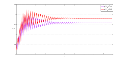
(b)
It is obvious that conditions (3.2),(3.25) and (3.34) are satisfied. For the positive initial value wherever, Eq.(4.1) has the unique positive equilibrium ,(see Fig.1-Fig.2).
where

Example 4.2 Consider the parameters the Pielou’s system with exponential terms (1.6) is as follows,
| (4.2) |
For the positive initial value wherever, the solution of Eq.(4.2) .
The parameters meet that conditions (3.24) and (3.33) . It is obvious that is the globally asymptotic stable. (see Fig.3-Fig.4.).

(a)

(b)

5. Conclusions
(i) System(1.6) is always persistent and bounded for .
(ii) System(1.6) always has a zero equilibrium; If , and then (0,0) is global asymptotic stable.
(iii) If , System(1.6) has a unique positive equilibrium ; Moreover, if and ,then is global asymptotic stable.
Conflict of interest
The authors declare that they have no competing interests.
Acknowledgment
This work was financially supported by Guizhou Scientific and Technological Platform Talents ([2022]020-1), Scientific Research Foundation of Guizhou Provincial Department of Science and Technology([2020]1Y008, [2022]021, [2022]026), and Scientific Climbing Programme of Xiamen University of Technology (XPDKQ20021).
Reference
[1] M. Kot, Elements of Mathematical Ecology , Cambridge University Press, New York, 2001.
[2] R. Beverton and S. Holt, On the dynamics of exploited fish populations, Fisheries Investigations, Ser 2, , 19 (1957), 1–533.
[3] MDL. Sen, The generalized Beverton-Holt equation and the control of populations, Applied Mathematical Modelling , 32 (2008), 2312-2328.
[4] X. Ding, W. Li , Stability and bifurcation of numerical discretization Nicholson blowflies equation with delay , Discrete Dyn. Nat. Soc , 2006 (2006), 1-12. Article ID 19413.
[5] A.J. Nicholson , An outline of the dynamics of animal populations , Aust. J. Zool , 2 (1954), 9-65 .
[6] E. C. Pielou, An Introduction to Mathematical Ecology , John Wiley Sons, New York, 1965.
[7] E. C. Pielou, Population and Community Ecology, Gordon and Breach , New York, 1974.
[8] Camouzis, E. , Ladas, G. Periodically forced Pielou’s equation, J. Math. Anal. Appl, 333(1) (2007), 117-127.
[9] Kulenovi, M.R.S. , Merino, Stability analysis of Pielou’s equation with period-two coefficient, J. Difference Equ. Appl, 13(5) (2007), 383-406.
[10] Ishihara, Keigo; Nakata, Yukihiko, On a generalization of the global attractivity for a periodically forced Pielou’s equation , J. Difference Equ. Appl. 18(3) (2012),375-396.
[11] Zhao, Houyu Analytic invariant curves for an iterative equation related to Pielou’s equation , J. Difference Equ. Appl. 19 (2013), no. 7, 1082-1092.
[12] Nyerges, Gabor, A note on a generalization of Pielou’s equation , J. Difference Equ. Appl. 14(5) (2008), 563-565.
[13] E. El-Metwally, E.A. Grove, G. Ladas, R. Levins, M. Radin, On the difference equation , Nonlinear Anal, 47 (2001), 4623-4634.
[14] I. Ozturk, F. Bozkurt, S. Ozen, On the difference equation , Appl. Math. Comput, 181 (2006), 1387-1393.
[15] Papaschinopoulos, G.; Ellina, G.; Papadopoulos, K. B. , Asymptotic behavior of the positive solutions of an exponential type system of difference equations , Appl. Math. Comput, 245 (2014), 181-190.
[16] Papaschinopoulos, G.; Radin, M. ; Schinas, C. J. , Study of the asymptotic behavior of the solutions of three systems of difference equations of exponential form , Appl. Math. Comput, 218 (2012), 5310-5318.
[17] A. Matsumoto, F. Szidarovszky, Asymptotic behavior of a delay differential neoclassical growth model , Sustainability, 5 (2013), 440-455.
[18] X. Ding, R. Zhang , On the difference equation , Adv. Difference Equ , 2008 (2008), http://dx.doi.org/10.1155/2008/876936. 7pages.
[19] L. Shaikhet, Stability of equilibrium states for a stochastically perturbed Mosquito population equation , Dyn. Contin. Discrete Impuls. Syst. Ser. B Appl.Algorithms , 21 (2) (2014), . 185-196.
[20] T. Awerbuch, E. Camouzis, G. Ladas, R. Levins, E.A. Grove, M. Predescu , A nonlinear system of difference equations , linking mosquitoes, habitats and community interventions , Commun. Appl. Nonlinear Anal , 15 (2) (2008) 77-88.
[21] B. Iricanin, S. Stevic, On two systems of difference equations , Discrete Dyn. Nat. Soc , 4 (2010) . (Article ID 405121).
[22] G. Papaschinopoulos, N. Fotiades, C.J. Schinas, On a system of difference equations including exponential terms , J. Difference Equ. Appl , 20 (5-6) (2014), 717-732.
[23] MDL Sen, S. Alonso-Quesada, Control issues for the Beverton-Holt equation in ecology by locally monitoring the environment carrying capacity: Nonadaptive and adaptive cases, Applied Mathematics and Computation , 215 (2009), 2616-2633.
[24] M. Bohner, S. Streipert, Optimal harvesting policy for the Beverton-Holt model, Mathematical Biosciences and Engineering , 13 (2016), 673-695.
[25] V. L. Kocic, G. Ladas, Global behavior of nonlinear difference equations of higher order with application , Kluwer Academic Publishers, Dordrecht, 1993.
[26] M. R. S. Kulenonvic, G. Ladas, Dynamics of second order rational difference equations with open problems and conjectures , Chapaman Hall/CRC,Boca Raton, 2002.
[27] Khan, A. Q.; Qureshi, M. N., Behavior of an exponential system of difference equations , Discrete Dyn. Nat. Soc, Art. ID 607281, 9 pp (2014).
[28] Papaschinopoulos, G.; Fotiades, N. ; Schinas, C. J., On a system of difference equations including negative exponential terms , J. Difference Equ. Appl., 20 (2014), 717-732.
[29] W. Chen, W. Wang, Global exponential stability for a delay differential neoclassical growth model , Adv. Difference Equ., 2014 (2014), 325.
[30] L. Shaikhet , Lyapunov Functionals and Stability of Stochastic Functional Differential Equations , Springer , Dordrecht, Heidelberg, New York, London,
[31] Enatsu, Y, Nakata, Y, Muroya, Y, Global stability for a class of discrete SIR epidemic models , Math. Biosci. Eng., 7 (2) (2010), 347-361.