Dynamic quantized consensus under DoS attacks:
Towards a tight zooming-out factor
Abstract
This paper deals with dynamic quantized consensus of dynamical agents in a general form under packet losses induced by Denial-of-Service (DoS) attacks. The communication channel has limited bandwidth and hence the transmitted signals over the network are subject to quantization. To deal with agent’s output, an observer is implemented at each node. The state of the observer is quantized by a finite-level quantizer and then transmitted over the network. To solve the problem of quantizer overflow under malicious packet losses, a zooming-in and out dynamic quantization mechanism is designed. By the new quantized controller proposed in the paper, the zooming-out factor is lower bounded by the spectral radius of the agent’s dynamic matrix. A sufficient condition of quantization range is provided under which the finite-level quantizer is free of overflow. A sufficient condition of tolerable DoS attacks for achieving consensus is also provided. At last, we study scalar dynamical agents as a special case and further tighten the zooming-out factor to a value smaller than the agent’s dynamic parameter. Under such a zooming-out factor, it is possible to recover the level of tolerable DoS attacks to that of unquantized consensus, and the quantizer is free of overflow.
I Introduction
Consensus of multi-agent systems has a variety of applications such as distributed computation, collaborative surveillance, sensor fusion and vehicle platoon [1]. Sophisticated devices such sensors, micro computers and wireless communication blocks are embedded in each agent, which can significantly promote the performance of consensus and make cooperation among agents possible. However, the challenges of malicious cyber attacks causing malfunctions also emerge, such as deceptive attacks and Denial-of-Service (DoS) attacks [2, 3]. Deceptive attacks influence the integrity of data and DoS attacks can induce malicious packet drops by radio-frequency interference and/or flooding the target with an overwhelming flux of packets to name a few.
In this paper, we are interested in a consensus problem of multi-agent systems under quantized data and malicious packet dropouts induced by DoS attacks. The quantizer has finite levels and quantization range. By controller design, we need to ensure that the quantizer should not saturate. Such problem is not trivial because, for example, if a dynamical agent’s measurements drift/diverge during packet-dropping intervals, some measurements may exceed the range of the quantizer.
The problems of packet dropouts have been well studied in the last two decades, e.g. in [4] for stochastic packet losses, and the case of DoS attacks inducing malicious packet dropouts has been investigated in [5, 6, 7, 8, 9]. For multi-agent systems under malicious packet dropouts, there are some recent developments for consensus, output regulation and formation control [10, 11, 9, 12]. Single integrator multi-agent systems under DoS attacks were studied in the papers [10, 13]. The objective therein is practical state consensus. Specifically, in [10], by self-triggered control, the nodes can achieve practical consensus if the number of consecutive packet losses is finite. In [13], by proposing randomized transmissions, the nodes are shown to achieve practical consensus even under frequent DoS attacks. For dynamical agents in a general form, the work [11] is one of the early papers considering consensus problems under DoS attacks by event-triggered control. The authors in [14] propose a novel distributed resilient control method without the pre-knowledge of the leader to solve the practical cooperative output regulation problem for multi-agent systems under DoS attacks. In [12], formation control of nonlinear multi-agent systems in the presence of malicious packet dropouts induced by DoS attacks is investigated. In [15], the authors consider asynchronous DoS attacks, i.e., the attacker is able to launch independent DoS attacks on communication edges.
Wireless communication for data transmission is widely used in cyber-physical systems. Despite the advantages of wireless communication such as remote transmission and lower costs for mass devices, the “competition” among devices for bandwidth resources may become overwhelming. Such competition would induce problems (e.g., delay and packet losses) to those control systems with large amounts of data exchange, e.g., large-scale multi-agent systems and sensor networks. Under limited bandwidth, signals can be subject to coarse quantization, and the consequence of quantization on control/measurement signals needs to be taken into account at the design stage. Static and dynamic quantizations have been proposed for various control problems. Centralized control systems under quantized communication have been extensively studied in the last two decades, for example by the seminal papers [16, 17]. Dynamic quantization with zooming-in and out is necessary to ensure quantizer unsaturation and asymptotic stability [18], where in particular the zooming-out factor should be able to compensate the influence of state divergence during open-loop control intervals, e.g., it should be “larger” than the unstable eigenvalues in case of a discrete-time system [4]. Centralized systems under dynamic quantization and DoS-induced packet losses have been studied in [7, 19]. In general, it is difficult to make the zooming-out factor equal to or smaller than the unstable eigenvalues because the state or estimation error can diverge at the rate of the unstable eigenvalues under open-loop mode (due to packet losses or sampled data control).
Dynamic quantization has also been extended to multi-agent systems without packet losses [20, 21, 22, 23]. In such works, quantized systems are equipped with zooming-in capability to ensure finite data-rate quantization and asymptotic convergence. When multi-agent systems are subject to DoS attacks and limited data-rate quantization, the recent paper [24] provides a design of dynamic quantization with both zooming-in and out capabilities to ensure quantizer unsaturation and consensus.
For multi-agent systems, when dynamic quantization due to limited data rate and packet losses coexist, one may have a question: Can we make the zooming-out factor tight and directly link it to the agent dynamics, e.g., lower bounded by the unstable eigenvalues of the open-loop system dynamic matrix? As mentioned before, such a problem has been well addressed for centralized systems [16, 4], but it is still open for multi-agent systems. Moreover, a tight zooming-out factor is meaningful because it can promote the multi-agent systems’ resilience against DoS attacks [24, 25].
In this paper, we provide a new design of dynamic quantized controller for output feedback multi-agent systems under DoS attacks. In the following, we compare our paper with the relevant literature in order to clarify our contributions. Generally speaking, the most relevant paper is our previous work [24]. In [24], the connections of zooming-out factor to the spectral radius of the open-loop system dynamic matrix of the agent are not explicit during the computation, and its value is conservative. It is also computationally intense in the sense that it needs matrix calculations of “high” dimensions (i.e. multi-agent’s state dimension times the total number of agents) for as many rounds as the number of the maximum consecutive packet losses. This also implies that one needs to know that number before controller design. By contrast, by the new control design in this paper, to obtain the zooming-out parameter, one only needs to calculate the spectral radius of the agent system matrix, and chooses a value larger than it. The information about the maximum DoS-induced packet losses is not needed. Moreover, an observer is implemented in this paper for handling output feedback while [24] does not involve state observation. From the viewpoint of technical analysis by switched system theory, this paper is more involved for having four modes, while [24] has only two modes. Compared with [10], our paper additionally takes limited data rate and the induced quantizer overflow problem into consideration. Moreover, the model of multi-agent systems in [10] takes the form of a single integrator, in which consensus error does not diverge even in the presence of DoS attacks. In our paper, the model of multi-agent systems is more general, which can incorporate open-loop unstable dynamics. Technically, it is more challenging to achieve consensus for multi-agent systems with unstable dynamics under DoS, not to mention under finite-level quantization. Compared with [11], our paper additionally considers quantized control under DoS, though transmissions are periodic and not based on event-triggered control.
In view of the comparisons mentioned above, we summarize the main contributions of this paper:
a) We develop a new output feedback quantized controller design for multi-agent systems, in which the bound of zooming-out factor is tight and directly linked to the agent dynamics compared with [24]: it is lower bounded by the spectral radius of the agent’s system matrix. Sufficient conditions on quantization range for overflow prevention and DoS attack for consensus are provided.
b) For scalar multi-agent systems, beyond the results of general linear multi-agent systems in a), we provide an approach to find a tighter zooming-out factor smaller than the agent’s system dynamic parameter. Under such a zooming-out factor, the bound of tolerable DoS attacks under unquantized consensus is recovered, and the quantizer is not saturated.
This paper is organized as follows. In Section II, we introduce the framework consisting of multi-agent systems and the class of DoS attacks. Section III contains two parts: general multi-agent systems as the main part and scalar multi-agent systems as a special case. A numerical example is presented in Section IV, and finally Section V ends the paper with concluding remarks and future research.
Notation. We denote by the set of reals. Given , and denote the sets of reals no smaller than and reals greater than , respectively; and represent the sets of reals no larger than and reals smaller than , respectively; denotes the set of integers. For any , we denote . Given a vector and a matrix , let and denote the - and -norms of vector , respectively, and and represent the corresponding induced norms of matrix . Moreover, denotes the spectral radius of . Given an interval , denotes its length. The Kronecker product is denoted by .
II Framework
Communication graph. We let graph denote the communication topology among agents, where denotes the set of agents and denotes the set of edges. Let denote the set of the neighbors of agent , where . In this paper, we assume that the graph is undirected and connected, i.e. if , then . Let denote the adjacency matrix of the graph , where if and only if and . Define the Laplacian matrix , in which and if . Let () denote the eigenvalues of and in particular we have due to the graph being connected. Let denote an identity matrix with dimension .
II-A System description
The agents interacting over the network are homogeneous linear multi-agent systems with sampling period :
| (1a) | ||||
| (1b) | ||||
where , , , and . We assume that is stabilizable and is observable. denotes the state of agent and denotes the output. We assume that an upper bound of the initial condition is known, i.e. [20, 21, 22]. Here, can be an arbitrarily large real as long as it satisfies this bound. This is for preventing the overflow of state quantization at the beginning. Let denote the control input, whose computation will be given in (12).
We introduce the control objective of this paper: State consensus. The average of the states is computed as and state consensus is defined by
| (2) |
It is trivial that (2) also implies the consensus of output . We assume that the spectral radius . Otherwise, consensus (2) is trivially achieved by setting for all .
In this paper, the communication channel for information exchange is bandwidth limited and subject to DoS. We assume that the transmission attempts of each agent take place periodically at time with and free of delay. Agent can only exchange quantized information with its neighbor agents over the network due to bandwidth constraints. In the presence of DoS, transmission attempts fail. We let represent the instants of successful transmissions. Note that is the instant when the first successful transmission occurs. Also, we let denote the time instant . In the remainder of the paper, we let represent instant , and represent instant () for the ease of notation.
Uniform quantizer. Let be the original scalar value before quantization and be the quantization function for scalar input values as
| (7) |
where is to be designed and , and . If the quantizer is unsaturated such that , then the error induced by quantization satisfies
| (8) |
Moreover, we define the vector version of the quantization function as , where with . It is clear that can be properly quantized if . In the remainder of the paper, by quantizer overflow or saturation, we mean that at least a exceeds the range of quantization, i.e., or equivalently .
II-B Time-constrained DoS
In this paper, we refer to DoS as the event for which all the encoded signals cannot be received by the decoders and it affects all the agents. We consider a general DoS model developed in [5] that describes the attacker’s action by the frequency of DoS attacks and their duration. Let with denote the sequence of DoS off/on transitions, that is, the time instants at which DoS exhibits a transition from zero (transmissions are successful) to one (transmissions are not successful). Hence, represents the -th DoS time-interval, of a length , over which the network is in DoS status. If , then takes the form of a single pulse at . Given with , let denote the number of DoS off/on transitions over , and let be the subset of where the network is in DoS status.
Assumption 1
(DoS frequency) [5]. There exist constants and such that for all with .
Assumption 2
(DoS duration) [5]. There exist constants and such that for all with .
Remark 1
Assumptions 1 and 2 do only constrain a given DoS signal in terms of its average frequency and duration. By [26], can be considered as the average dwell-time between consecutive DoS off/on transitions, while is the chattering bound. Assumption 2 expresses a similar requirement with respect to the duration of DoS. It expresses the property that, on the average, the total duration over which communication is interrupted does not exceed a certain fraction of time specified by . Like , the constant is a regularization term. It is needed because during a DoS interval, one has . Thus serves to make Assumption 2 consistent. Conditions and imply that DoS cannot occur at an infinitely fast rate and be always active.
The lemma below presents the relation between the number of successful transmissions and the number of transmission attempts . Let and denote the numbers of successful and unsuccessful transmissions between steps 1 and , respectively.
Lemma 1
[7] Consider the DoS attacks in Assumptions 1 and 2 and the network sampling period . If , then
III Main results
III-A Control architecture
To deal with output feedback, an observer estimating from is locally implemented at agent given by
| (9) |
where denotes the observer state and . Since is observable, there exists a matrix such that the spectral radius . Then, is quantized and transmitted to the neighbors. Let denote the decoded value of by agent and vice versa for , whose computations will be given later.
For agent , the control input has two modes aligned with the status of DoS:
| (12) |
for . Let . Note that each agent is able to passively know the status of DoS at by whether receiving neighbors’ transmissions or not. We assume that there exists a feedback gain such that the spectral radius of
| (13) |
satisfies , where denotes the eigenvalues of . Note that is needed to achieve consensus even if DoS is absent. The assumption on the existence of is motivated by the consensusability of linear discrete-time multi-agent systems [20]. If DoS is absent and precise information is available, a sufficient condition to ensure the existence of is that where represents unstable eigenvalues of .
In our paper, the encoder and decoder for each state have the same structure. In the following, we first explain the decoding process. In (12), is the decoded value of () at the decoder of agent with initial condition . Its computation is given by
| (16) |
in which , and is the value generated and transmitted by the encoder of agent given by
| (17) |
The computation of in the decoder of agent follows
| (20) | |||
| (21) |
Now we explain the synchronization of a decoded state among agents, that is, for , the values of , and are identical for all . This is because the decoders of agents and have the same initial condition (), have the same and receive the same in , and for all . The synchronization of in the decoders and also in the encoders will be explained after (31). Thus, the superscripts of , and can be omitted, and it is enough to let represent the decoded value of in the decoders. At last, we point out that the encoder is a copy of the decoder, and thus one has that in the encoder also has the same value as in the decoders.
Therefore (12) can be rewritten as
| (24) |
and (16) and (20) can be rewritten as
| (27) |
in which , with . Similarly, (17) and (21) can be written as
| (28) |
The switched-type estimator in (27) has the following motivations. The first equation in (27) is for acquiring the quantized information of under successful transmissions, and then calculates . This step is also necessary for the DoS-free case [20]. The second equation in (27) is an open loop estimation, and it together with the second equation in (24) can decouple the state of the agents and the quantization errors (see Case d) later).
A key parameter in (28) is the scaling parameter . By adjusting its value dynamically, the variable to be quantized will be kept within the bounded quantization range without saturation. The scaling parameter is updated as
| (31) |
with . The parameters and are the so-called zooming-in and out factors in dynamic quantization, respectively. Since in the encoders and decoders has the same initial condition , and or is passively known as mentioned before, one can see that is synchronized in all the encoders and decoders. The zooming-in and out mechanism in (31) is majorly inspired by [4, 7] studying centralized systems. The scaling parameter is a dynamic sequence whose increasing and decreasing depend on DoS attacks in order to mitigate the influence of DoS-induced packet losses. If one assumes that each agent is aware of its own and their neighbors’ (), it is possible to design distributed zooming-in factors, namely . Then the new and are complicated and will be a vector and a matrix, respectively. This case will be left for future research. The design of zooming-out factor may not change since it is dependent on (see Lemma 2 later).
During DoS intervals, in (28) may diverge. Therefore, the scaling parameter must increase using so that is not saturated. If the transmissions succeed, the quantizers zoom in and decreases by using . The selections of and will be specified later, and one of the objectives of this paper is to find a as tight as possible. If one assumes that the communication network is free from any DoS-induced or random packet losses, then the zooming-out mechanism is not necessary since in does not diverge. In this case, one only needs the zooming-in mechanism to ensure the property of asymptotic convergence [20, 22].
By defining vectors , one can obtain the compact form of (27) as
| (34) |
for . The compact form of the observer in (III-A) is
| (35) |
in which , , , , and . Let . With the vectors and , we define the following errors in vector form
in which denotes the error due to signal coding and denotes the observer error. From (1), one can see that the update of is independent on or . However, the update of depends on or , due to the control law in (24). Note that such dependence does not exist in [24]. One can obtain the compact form of the closed-loop dynamics of as
| (38) |
where and Let the discrepancy between the state of agent and be and let . Then one can obtain the compact dynamics of :
| (41) |
It is clear that if as , consensus of the multi-agent system is achieved as in (2). If the multi-agent system is subject to DoS, has a diverging mode by the second equation in (III-A), and the dynamics of and are not clear, which implies that consensus may not be achieved.
Note that the control system in this paper looks similar but different from the common “to zero” static controller, i.e., the control input is set to zero under DoS attacks, see [10]. The controller design in our paper is also different from the “pure” prediction based controller in lossy networks (i.e., is always computed based on the state prediction) in [24, 11]. In our paper, the decoder (27) generates () regardless of the presence of DoS. Meanwhile, the input is set to zero and does not depend on the estimated state when , though is available. However, computing under DoS is necessary since its value is useful when DoS is over. Consequently, as will be shown later, the technical analysis involves four modes by expressing the overall system as a switched system. By contrast, the analysis in [24] needs to consider only two modes.
III-B Dynamics of the multi-agent systems
Though the update of in (III-A) depends on the previous step, i.e., or , the update of is affected by both the and -th steps. This is because in (III-A) depends on or , and in (34) depends on or . To make the technical analysis approachable, we conduct the analysis by four cases:
Case a) In view of in the first equation of (34) and in (III-A), one can obtain , in which we have
| (42) |
with and . One can also compute the estimation error in the observer
| (43) |
in which the spectral radius due to . Recall the update of for in (III-A). Then by (III-A)–(43), one obtains the dynamics of , and as follows:
| (44a) | |||
| (44b) | |||
| (44c) | |||
Case b) In view of in the first equation in (34) and in (III-A), where due to , one can obtain that The dynamics of for Case b) follows from the second equation in (III-A). The control input applied to the observer is also due to , which implies that (44c) still holds. With above, one obtains the dynamics of , and as
| (45a) | |||
| (45b) | |||
| (45c) | |||
Case c) By substituting the dynamics of in the second equation of (34), one has the evolution of as The dynamics of in (43) also holds in this case. In view of the dynamics of in the first equation of (III-A), overall one can obtain that
| (46a) | ||||
| (46b) | ||||
| (46c) | ||||
Case d) For computing , by in the second equation of (34) and in (III-A) with due to , one can have The dynamics of in (43) still holds in this case. Then, by combining the dynamics of in the second equation of (III-A), we can obtain that
| (47a) | ||||
| (47b) | ||||
| (47c) | ||||
To further facilitate the analysis, we define three new variables:
| (48) |
where has been given in (31). The dynamics of , and corresponding to the four cases above, respectively, are presented in the following:
Case a)
| (49a) | |||
| (49b) | |||
| (49c) | |||
Case b)
| (50a) | |||
| (50b) | |||
| (50c) | |||
Case c)
| (51a) | |||
| (51b) | |||
| (51c) | |||
Case d)
| (52a) | |||
| (52b) | |||
| (52c) | |||
III-C Quantized consensus
Since is observable by assumption, we can choose an observer gain such that . Now we present a technical lemma concerning the upper bound of .
Lemma 2
Proof. We start the analysis from a successful transmission instant (). If the next instant (corrupted by DoS), one can see that this scenario ( and ) corresponds to Case c), and one can obtain by (51a). If as well, this scenario ( and ) corresponds to Case d). Then according to (52a), one can obtain . By iteration, it is straightforward that if all the transmissions at fail, then
| (57) |
where the last equality is obtained by substituting in (51a). If is an instant of successful transmissions, namely , then by (50a) in Case b) and (III-C), one has that . By switching the in with the in and , and recalling that and , one has
| (58) |
where denotes the number of consecutive unsuccessful transmissions between and . If there is no DoS attack between and , i.e., , then (III-C) is recovered to (49a).
There exists a unitary matrix given by
| (59) |
where with satisfies and . With such , we let
in which , and denote vectors composed by the first elements in , and , respectively. Then, by (III-C), one can obtain
| (60) |
in which the last equality is obtained by the fact that and are commuting matrices: One can verify that for all . It is also easy to verify that . Note that and are block diagonal matrices, thus, from (III-C), one can obtain the dynamics of as
| (61) |
in which . One can verify that (III-C) also holds for . By the iteration of (III-C), one can obtain
| (62) |
where we let when in the second line.
Let and () denote the numbers of successful and unsuccessful transmissions within the interval , respectively. Note that and as defined after (54) always exist. Then, in view of the first line in (III-C), one can obtain
| (63) |
in which by the selections of and , and by (54). Hence, by (III-C), we have
| (64) |
in which by (75) in [24]. Note that By assumption, we have for . Incorporating , overall for , one has and hence
| (65) |
By the dynamics of in Cases a)–d), we have
| (66) |
in which , by the selection of and . By (III-C), one has
| (67) |
Note that in (III-C), and with . Substituting (III-C) and (III-C) into (III-C), we have
| (68) |
Then, one has . Trivially, (III-C) also holds for .
Remark 2
The upper bound of is influenced by the frequency of DoS attacks shown by (54), and therefore influences , which determines the necessary data rate (see Theorem 1 later). DoS frequency influences due to the nature of switching in the system, e.g., can diverge under fast switches among Cases a)-d) due to fast off/on of DoS attacks. As will be shown later, in case of scalar multi-agent systems, DoS-frequency constraint in (54) does not influence the problem any more.
Remark 3
We emphasize that in Lemma 2 is lower bounded by , and it is tighter than that in [24]. We explain how the new controller can attain this. One of the major functions of the new controller is to obtain Case d), in which and in (52) are decoupled under DoS and regulated by . If one adopts the controller in [24], and are coupled under DoS attacks. This implies that one can not simply multiply by in (III-C). Instead, one needs to simultaneously consider and due to the couplings, and obtains a form similar to (III-C) but should be replaced by a matrix derived from the combinations of , and . Then, to obtain from , one needs to remove some lines and rows of the matrix [24], and hence loses its connections to . Eventually, in order to obtain a realizing zooming-out, one needs to take the worst-case analysis (i.e., consider all the possible scenarios of consecutive packet losses and compute the corresponding , then select the largest ), and this is the major reason of conservative and inexplicit in [24]. This is also computationally intense.
Remark 4
Compared with the results in [24], the parameters and in this paper can be directly selected when and are known, respectively. In contrast, the choices of and in [24] need complex calculations including matrix multiplication and taking their norms for as many rounds as the number of maximum consecutive packet losses (see Lemma 3, [24]). That is to say, one needs to know the maximum number of consecutive packet drops in order to compute . By contrast, to obtain in this paper, such information is not needed and one only needs to compute and then selects a tight value provided that (54) holds. To attain the above merits of the new controller over those in [24], one needs to deal with a stabilization problem of a switched system of four modes (i.e, Cases a)-d)) in the technical analysis, instead of two modes in [24]. As will be shown later in the proof of Theorem 1, the four-mode switched system also complicates the calculation of data rate.
In general, it is difficult to tighten the zooming-out factor beyond the eigenvalues of open-loop systems. This aspect can be more clearly discussed for centralized systems. For example, in the paper [4] considering a discrete-time system, the quantization needs to zoom out with the factor of (the -th unstable eigenvalue of ) for each failed transmission in order to “catch” the diverging estimation error. Similarly, for a continuous-time system, the zooming-out factor is continuous (real part of : Re) during open-loop intervals [7]. For multi-agent systems, the lack of global state is another challenge. The results mentioned for centralized systems significantly depend on designing a fine predictor having access to the entire state. However, such a predictor is not applicable to multi-agent systems because of the distributed system structure where the agents are constrained to have only local information of their direct neighbors. Therefore, in [24], the authors attempt to predict the state by an open-loop estimator and feed the estimations to the feedback controller. However, due to matrix manipulations, the zooming-out factor eventually loses its connections to the eigenvalues of .
In the following, we present the main result of the paper.
Theorem 1
Consider the multi-agent system (1) with control inputs (III-A) to (31), where and are selected as in Lemma 2. Suppose that the DoS attacks characterized in Assumptions 1 and 2 satisfy (54). If in the quantizer (7) satisfies
| (69) |
where and , then quantizer (7) is not overflowed. Moreover, if DoS attacks satisfy
| (70) |
then consensus of is achieved as in (2). The parameter in is chosen such that (), where
| (73) |
Proof. The unsaturation of quantizer is proved by induction: if the quantizer satisfying (69) is not overflowed such that for and recall that , then the quantizer will not saturate at the transmission attempts within the interval and hence .
a) In the proof, represents an instant of successful transmission () or the initial time . At , the quantized information of attempts to transmit through the network, i.e., In order to prevent quantizer overflow, must be upper bounded by the maximum quantization range, i.e., . By (III-B), one has
| (74) |
One can verify that the quantizer at is not saturated since in (69), where by Lemma 2, and in (III-C).
b) At , quantized signals of attempt to be transmitted to the decoders, and one needs to compute However, one cannot compute it directly as in a) because has two cases: the transmission attempts at in a) are successful or corrupted by DoS. b-1) If , then one can apply the similar analysis in a) and concludes that does not saturate at . b-2) If the transmission attempts at in a) are not received by the decoders, then at , by (III-B) with , one can compute that
| (76) |
in which by (51) one has
| (78) | ||||
| (84) |
By (III-C), (78) and the upper bounds of and in a), one can verify that in (69).
c) By b-1), if the previous step is not under DoS, one can always follow a) to verify quantizer unsaturation. Hence, we omit this case and analyze consecutive packet losses until . At , one should focus , in which by (52) one can obtain
| (89) |
with in (78). Substituting (78) and (89) into , one can verify that quantizer is not saturated at by
| (92) | ||||
| (93) |
where defined below (70) exists since .
By the analysis in a)–c), one can conclude that the quantizer does not saturate during with . This implies that the quantizer does not saturate at all .
d) Now we show state consensus. We first need to prove that is finite for all . For this, it is sufficient to show is bounded during . We have proved that and are upper bounded by Lemma 2. Then, we only need to show is bounded for . If is a failed transmission instant, by (51a), one can infer that is upper bounded. One can also infer that is also upper bounded in view of by (52a) with and . By the analysis above, we conclude that all the during is upper bounded and hence is finite for all . Recall the definitions of and before Lemma 1. In view of , one has where and by (70). Thus, we have as , which implies state consensus.
Remark 5
In principle, one can select arbitrarily close to and close to in order to improve the system resilience for reaching consensus in view of (70). Such choices are effective especially under long time but less frequent DoS attacks. However, such choices may also lead to larger and , respectively, and a smaller in (54). This implies that may diverge under frequent DoS attacks due to fast switches in a switched control system (see Remark 2). It is clear that a small can always relax the constraints in (54) and (70), but can increase the communication burden.
III-D Scalar multi-agent systems
If , one sees that overflow problem of quantizer is subject to dwell time constraint in (54). As mentioned before, the system is not subject to the constraint in case , i.e. a scalar multi-agent system. More importantly, in case , we are able to further tighten the zooming-out factor, i.e., smaller than and therefore recover the robustness result of unquantized control, i.e., if DoS attacks satisfy
| (94) |
consensus of is achieved and the quantizer is not saturated. We briefly present the proof of unquantized case obtaining (94) in the Appendix. In the following, we present the result of quantizer unsaturation and consensus for scalar multi-agent systems. We assume that and is directly known, since one can always obtain .
The controller in (24) to (31) is still applicable, and in (28) should be replaced by . Consequently, and for all .
Proposition 1
Consider the multi-agent system (1) with and the control inputs (24) to (31). Suppose that the DoS attacks characterized in Assumptions 1 and 2 satisfy . For any , the choice of should satisfy
| (95) |
then the followings hold:
-
(1)
the quantizer does not saturate if ( and are positive given in proof);
-
(2)
Moreover, if (94) holds, consensus of is achieved.
Proof. Note that in order to prove consensus by showing , one can follow the analysis in Lemma 2 and conclude is finite. One can obtain the dynamics of similar to (III-C), in which for all . Then the counterpart of (III-C) is given by
| (96) |
and the counterpart of (III-C) is given by As and are diagonal matrices, the stability of the switched system is free from the dwell time constraint in (54). In order to ensure the boundedness of , needs to be smaller than 1, which is implied by
| (97) |
The bounds of and obtained in the proof of Lemma 2 still hold. Then, one can obtain with .
At , the quantized information of attempts to transmit , and hence must be upper bounded by the maximum quantization range. Specifically, one has and the quantizer at is not saturated since
At , the quantized signals of needs to be transmitted to the decoders, and one needs to compute If the transmission attempts at are successfully received by the decoders, then one can apply the similar analysis in the former paragraph and then concludes that does not encounter the overflow problem at . If the transmission attempts at are not received by the decoders, then at , one can obtain
| (98) |
where the last equality is due to according to (51b), in which . By induction, if all the transmission attempts at fail, then one can obtain that at , the quantizer does not saturate since
| (99) |
in which . Here, denotes the maximum number of consecutive packet losses, and can be calculated by Lemma 2 in [24].
For showing consensus, one needs to prove as , in which can be shown upper bounded by following an analysis similar to that in Theorem 1. By (70), it holds that as . Overall, in order to achieve consensus and quantizer unsaturation simultaneously, DoS attacks need to satisfy
| (100) |
where the second term in is obtained by imposing in (97). One can verify that since and satisfy (95), it holds which leads to (94).
Remark 6
In order to preserve (94), given a , one needs to compute by (95). Otherwise, (94) cannot be preserved. One should notice that obtained by (95) is smaller than since . As a result, to obtain Proposition 1, we need the information of the maximum consecutive packet drops () in order to compute and therefore the necessary data rate by (III-D). However, if one lets , then the information of is not needed, while one could not recover (94), which implies a less robust system. One can verify that the right-hand side of (94) is always larger than that of (70), which implies a better robustness of a scalar multi-agent system than a general linear multi-agent system.

IV Numerical example
In the simulation example, we consider a multi-agent system of with
| (105) |
and s. The Laplacian matrix of the undirected and connected communication graph follows that in [27]. We select a feedback gain .
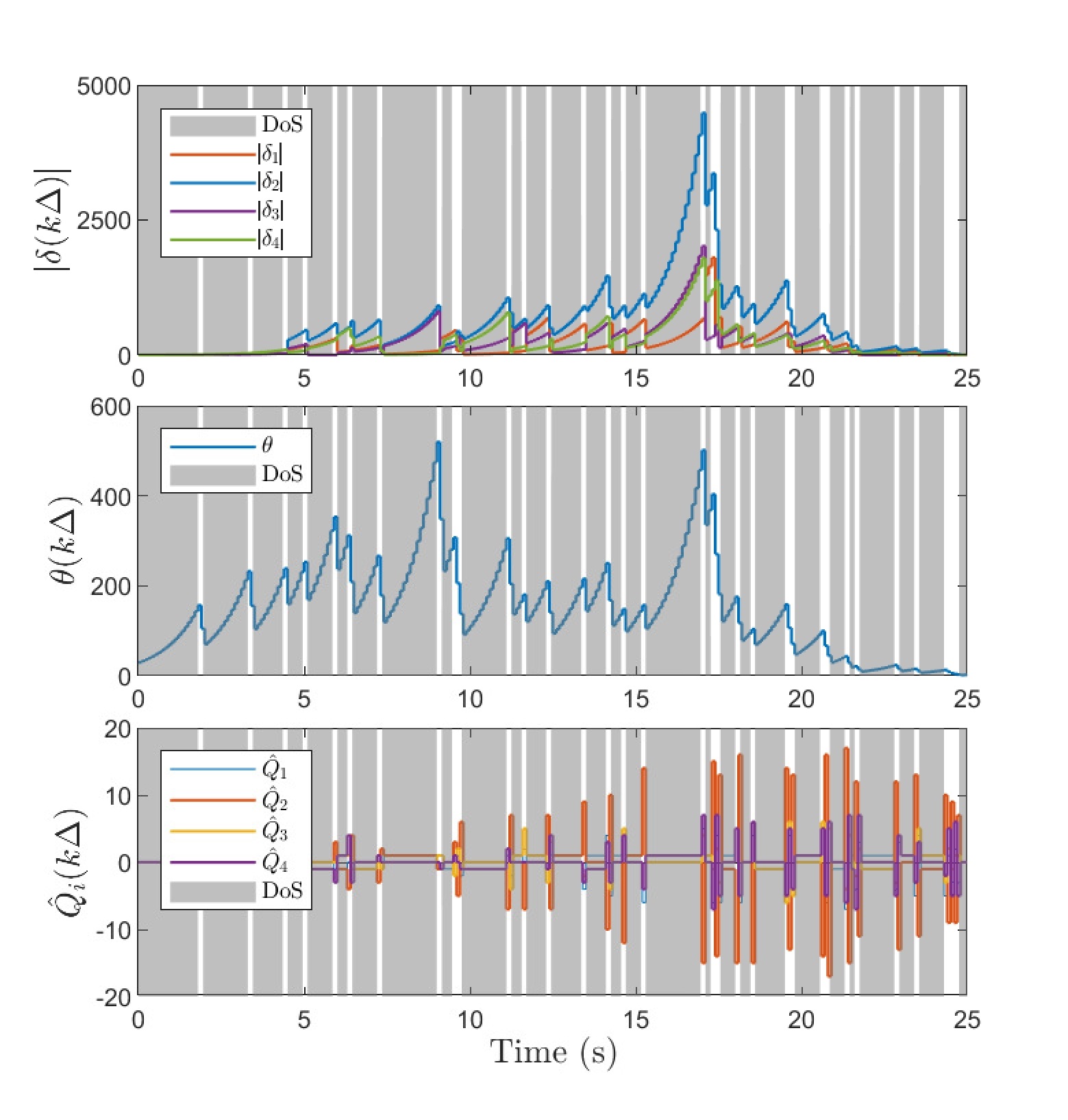
We consider a sustained DoS attack with variable period and duty cycle, generated randomly. Over a simulation horizon of s, the DoS signal yields s and . This corresponds to values (averaged over s) of and , and hence and .
Under this setting, one can obtain , , and . Then we select and according to Lemma 2. For the observer gain, we select with . One can verify that (in (III-C)). One can also see that (54) holds in view of and . By Theorem 1, we obtain the right-hand side of (69) being 301920.
Simulation plots are presented in Figure 1. We point out that the DoS frequency constraint (54) is satisfied in the simulation example, but the level of DoS attacks characterized by is stronger than the theoretical sufficient bound computed by (70), which is . Since our result regarding tolerable DoS attacks is a sufficient condition, one can see from the first and second plots in Figure 1 that state consensus is still achieved. When one increases to about , then the states and diverge. By the third plot in Figure 1, one can see that is a decreasing and increasing sequence during DoS-free and DoS time, respectively. Thanks to the dynamical , the quantizer is not overflowed, which can be seen from the last plot in Figure 1. Specifically, the quantization range provided by the theoretical value is much larger than the utilized quantization range in simulation. One could see that our sufficient condition for quantizer unsaturation is quite conservative. One of the reasons is that we have frequently used “” and in (III-C) for instance and for matrices and vectors in (III-C) for instance. Moreover, a small can also lead to a large data rate as discussed in [24]. Without DoS, such a conservativeness also exists in consensus under data rate limitation in [20, 21] for instance.
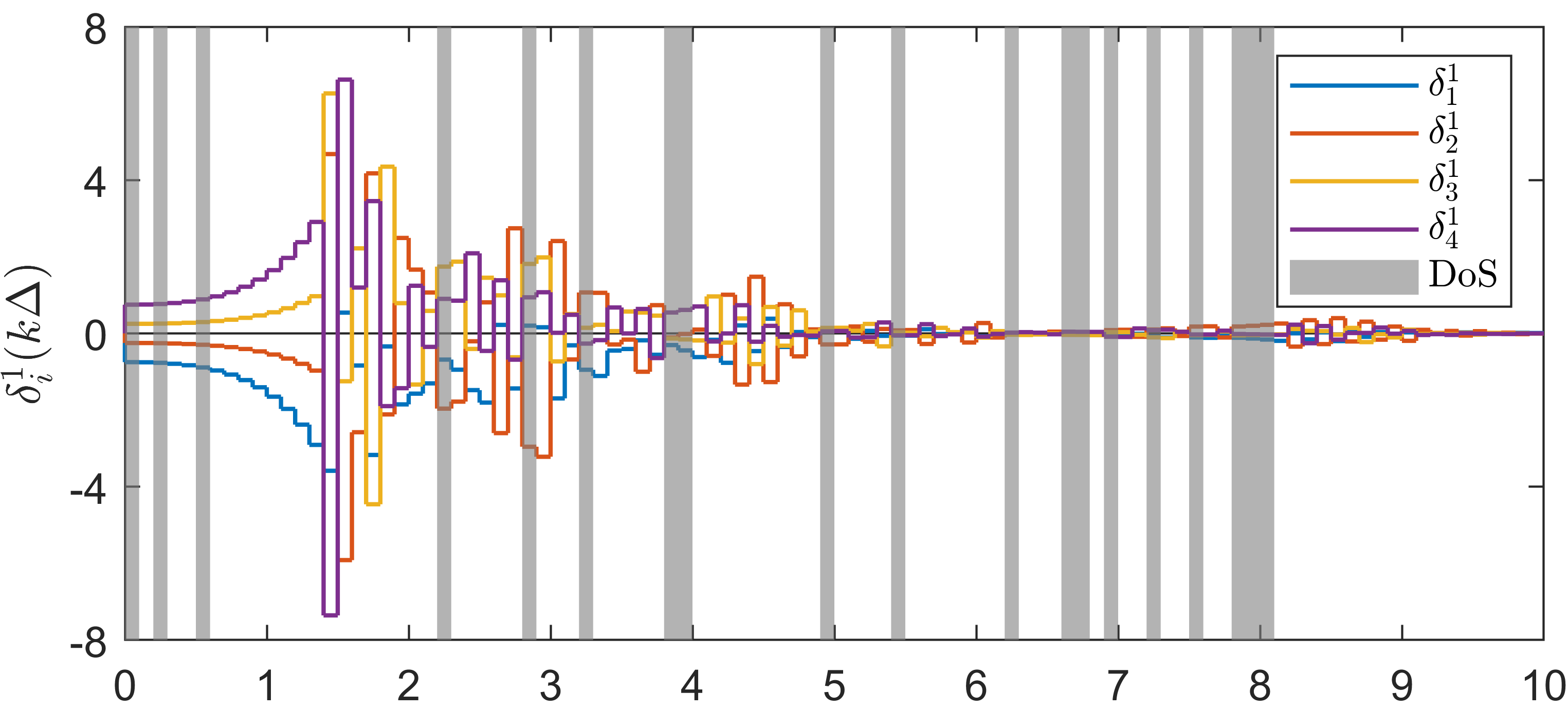
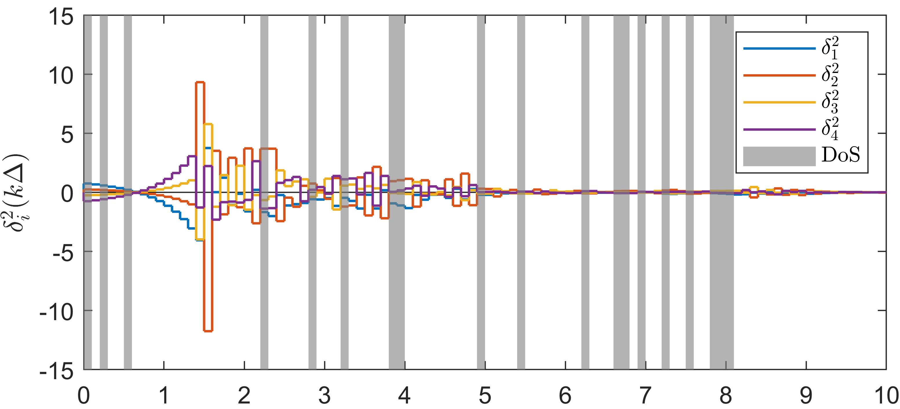
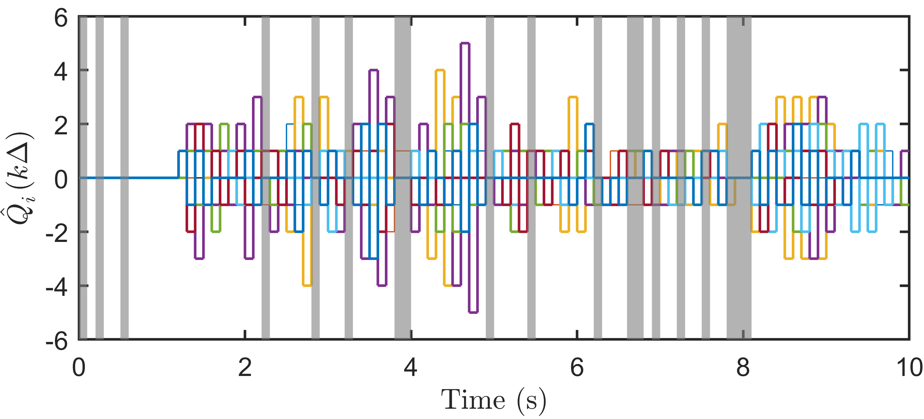
Scalar multi-agent systems: We consider the multi-agent system in the numerical example in [20], in which , and . The Laplacian matrix of the undirected and connected communication graph follows that in the previous example. We select and s. One has . According to Proposition 1, we choose and , and quantizer parameter should be no smaller than . Besides, the sufficient DoS condition for consensus is
| (106) |
Similar to the previous simulation example, the randomly generated DoS over a simulation horizon of s (gray stripes in Figure 2) yields s and . This corresponds to values (averaged over s) of and , and the DoS attacks in this example yield .
The simulation results are presented in Figure 2. The convergence of () is presented in the first plot of Figure 2, in which one can see increases during DoS intervals (gray areas) and decreases when DoS is not present (white areas). Note that implies the state consensus. The zooming-in and zooming-out mechanism can be observed by the second plot in Figure 2, in which increases and decreases during DoS present and absent intervals, respectively. The effectiveness of zooming-in and out mechanism is shown by the third plot of Figure 2. Though the state increases during DoS present intervals, with the zooming out of for mitigating the influence of DoS, one can see that the actual value of does not diverge under DoS. Importantly, compared with the and the DoS bound 0.2037 in [27], one can see that the zooming-out factor in this paper and the bound for tolerable DoS 0.8134 in (IV) are indeed much improved.
Conservativeness also exists in the case of scalar multi-agent systems, which can be seen by the gaps of DoS level between 0.8134 (theoretical sufficient bound in (IV)) and 0.9320 (actual DoS in the simulation), and the gaps between the theoretical quantization range and the utilized range shown in the third plot of Figure 2.
V Conclusions and future research
We have presented the results for quantized consensus of output feedback multi-agent systems. The design of dynamic quantized controller including the observer and the zooming-in and zooming-out parameters has been presented. The calculation of zooming-out factor is tight, whose lower bound is the spectral radius of the agent’s dynamic matrix. Moreover, the approach of this paper shows the explicit relations between the zooming-out factor and the agent dynamic matrix. We have also provided the bounds of quantizer range and tolerable DoS attacks. It has been shown that the quantizer is free of overflow during DoS intervals and the state consensus can be achieved. At last, as a special case of scalar multi-agent systems, we have shown that it is possible to further tighten the zooming-out factor and make it smaller than the agent’s system parameter without causing quantizer overflow. The resilience is also improved by such a zooming-out factor, i.e., recover to that of unquantized consensus under DoS.
Our work can be extended to various directions. Following [28], one can consider the control structure in which each agent directly exchanges output information with the neighbors by implementing a modified observer in the decoder. It is possible to extend our results to a directed graph of the communication topology, in which the analysis after Section III-C will need to be adapted [29]. Last but not least, it is meaningful to consider the case in which the decoded values of a state are different due to communication noise or parameter uncertainties for instance.
Proof for (94). In case and , it is easy to obtain directly from and an observer is not necessary. Hence, we assume that . In case of infinite data rate, one can obtain that With the unitary matrix in (59) and by , one can obtain that in which . Partition the vector , in which is the first component in the vector and is composed by the rest. Then we obtain the dynamics of as and therefore By the iteration of , one can obtain . Note that for all . Then one can obtain and . By substituting the bound in Lemma 1 into and , one can obtain that where . If the level of DoS attacks satisfy (94), then As , one has , which implies the consensus of .
References
- [1] F. Bullo, Lectures on Network Systems. Kindle Direct Publishing, 2019.
- [2] P. Cheng, L. Shi, and B. Sinopoli, “Guest editorial: Special issue on secure control of cyber-physical systems,” IEEE Transactions on Control of Network Systems, vol. 4, no. 1, pp. 1–3, 2017.
- [3] A. Teixeira, I. Shames, H. Sandberg, and K. H. Johansson, “A secure control framework for resource-limited adversaries,” Automatica, vol. 51, pp. 135–148, 2015.
- [4] K. You and L. Xie, “Minimum data rate for mean square stabilization of discrete lti systems over lossy channels,” IEEE Transactions on Automatic Control, vol. 55, no. 10, pp. 2373–2378, 2010.
- [5] C. De Persis and P. Tesi, “Input-to-state stabilizing control under Denial-of-Service,” IEEE Transactions on Automatic Control, vol. 60, no. 11, pp. 2930–2944, 2015.
- [6] A.-Y. Lu and G.-H. Yang, “Input-to-state stabilizing control for cyber-physical systems with multiple transmission channels under denial of service,” IEEE Transactions on Automatic Control, vol. 63, no. 6, pp. 1813–1820, 2017.
- [7] S. Feng, A. Cetinkaya, H. Ishii, P. Tesi, and C. De Persis, “Networked control under DoS attacks: Tradeoffs between resilience and data rate,” IEEE Transactions on Automatic Control, vol. 66, no. 1, pp. 460–467, 2021.
- [8] Y. Li, D. E. Quevedo, S. Dey, and L. Shi, “SINR-based DoS attack on remote state estimation: A game-theoretic approach,” IEEE Transactions on Control of Network Systems, vol. 4, no. 3, pp. 632–642, 2017.
- [9] C. Deng and C. Wen, “Distributed resilient observer-based fault-tolerant control for heterogeneous multiagent systems under actuator faults and DoS attacks,” IEEE Transactions on Control of Network Systems, vol. 7, no. 3, pp. 1308–1318, 2020.
- [10] D. Senejohnny, P. Tesi, and C. De Persis, “A jamming-resilient algorithm for self-triggered network coordination,” IEEE Transactions on Control of Network Systems, vol. 5, no. 3, pp. 981–990, 2017.
- [11] Z. Feng and G. Hu, “Secure cooperative event-triggered control of linear multiagent systems under DoS attacks,” IEEE Transactions on Control Systems Technology, vol. 28, no. 3, pp. 741–752, 2020.
- [12] Y. Tang, D. Zhang, P. Shi, W. Zhang, and F. Qian, “Event-based formation control for nonlinear multiagent systems under DoS attacks,” IEEE Transactions on Automatic Control, vol. 66, no. 1, pp. 452–459, 2021.
- [13] A. Cetinkaya, K. Kikuchi, T. Hayakawa, and H. Ishii, “Randomized transmission protocols for protection against jamming attacks in multi-agent consensus,” Automatica, vol. 117, p. 108960, 2020.
- [14] C. Deng, D. Zhang, and G. Feng, “Resilient practical cooperative output regulation for mass with unknown switching exosystem dynamics under DoS attacks,” Automatica, vol. 139, p. 110172, 2022.
- [15] A.-Y. Lu and G.-H. Yang, “Distributed consensus control for multi-agent systems under Denial-of-Service,” Information Sciences, vol. 439, pp. 95–107, 2018.
- [16] S. Tatikonda and S. Mitter, “Control under communication constraints,” IEEE Transactions on Automatic Control, vol. 49, no. 7, pp. 1056–1068, July 2004.
- [17] G. N. Nair and R. J. Evans, “Stabilizability of stochastic linear systems with finite feedback data rates,” SIAM Journal on Control and Optimization, vol. 43, no. 2, pp. 413–436, 2004.
- [18] D. Liberzon and D. Nesic, “Input-to-state stabilization of linear systems with quantized state measurements,” IEEE Transactions on Automatic Control, vol. 52, no. 5, pp. 767–781, 2007.
- [19] W. Liu, J. Sun, G. Wang, F. Bullo, and J. Chen, “Resilient control under quantization and Denial-of-Service: Co-designing a deadbeat controller and transmission protocol,” IEEE Transactions on Automatic Control, early access, 2022.
- [20] K. You and L. Xie, “Network topology and communication data rate for consensusability of discrete-time multi-agent systems,” IEEE Transactions on Automatic Control, vol. 56, no. 10, pp. 2262–2275, 2011.
- [21] T. Li, M. Fu, L. Xie, and J.-F. Zhang, “Distributed consensus with limited communication data rate,” IEEE Transactions on Automatic Control, vol. 56, no. 2, pp. 279–292, 2010.
- [22] C. Gao, Z. Wang, X. He, and H. Dong, “Fault-tolerant consensus control for multiagent systems: An encryption-decryption scheme,” IEEE Transactions on Automatic Control, vol. 67, no. 5, pp. 2560–2567, 2022.
- [23] Z. Qiu, L. Xie, and Y. Hong, “Quantized leaderless and leader-following consensus of high-order multi-agent systems with limited data rate,” IEEE Transactions on Automatic Control, vol. 61, no. 9, pp. 2432–2447, 2015.
- [24] S. Feng and H. Ishii, “Dynamic quantized consensus of general linear multiagent systems under Denial-of-Service attacks,” IEEE Transactions on Control of Network Systems, vol. 9, no. 2, pp. 562–574, 2022.
- [25] M. Ran, S. Feng, J. Li, and L. Xie, “Quantized consensus under data-rate constraints and DoS attacks: A zooming-in and holding approach,” IEEE Transactions on Automatic Control, pp. 1–16, DOI: 10.1109/TAC.2022.3 223 277, 2022.
- [26] J. P. Hespanha and A. S. Morse, “Stability of switched systems with average dwell-time,” in Proceedings of IEEE Conference on Decision and Control, 1999, pp. 2655–2660.
- [27] S. Feng and H. Ishii, “Dynamic quantized consensus of general linear multi-agent systems under Denial-of-Service attacks,” in Proceedings of IFAC World Congress, 2020, pp. 3533–3538.
- [28] Y. Meng, T. Li, and J.-F. Zhang, “Coordination over multi-agent networks with unmeasurable states and finite-level quantization,” IEEE Transactions on Automatic Control, vol. 62, no. 9, pp. 4647–4653, 2016.
- [29] Z. Chen, J. Ma, and X. Yu, “Consensus of general linear multi-agent systems under directed communication graph with limited data rate,” in Proceedings of International Symposium on Autonomous Systems, 2019, pp. 394–399.