Dynamic Properties of Two-Dimensional Latticed Holographic System

The DC conductivity $\sigma_{\text{DC}}$ can be obtained with horizon data. For an anisotropic background, the DC conductivity is anisotropic as well. Previous studies on anisotropy focused only on two distinct directions. To reveal more detailed anisotropic behavior of the DC conductivity, we study the DC conductivity along an arbitrary direction, i.e., the anisotropic DC conductivity.

In Fig. 1, we can find that the upper left plot and the upper right plot correspond to the insulating phase and metallic phases, respectively. For the lower row plots, the system is insulating in $x$-direction, while metallic in $y$-direction. Also, the intersection point in both plots of the lower row suggests that $\sigma_{x}=\sigma_{y}$ at certain temperature, which results in isotropic $\sigma$.

To obtain the anisotropic DC conductivity, we study the linear responses behaviors of the current

where $J_{i}$, $E_{j}$, $R_{ij}$ are current, electric field and response matrix, respectively. Following the method in Donos:2014uba (also see Blake:2014yla ; Ling:2016dck ), we can calculate the DC conductivity $\sigma_{x\mathrm{DC}},\sigma_{y\mathrm{DC}}$ along the $x,y$ direction, respectively

with the off-diagonal components $R_{12}=R_{21}=0$. Therefore the angle-dependent DC conductivity reads,

Once the DC conductivity is at hand, we can define the metallic phase as $\sigma^{\prime}_{DC}(\tilde{T})<0$ and the insulating phase as $\sigma^{\prime}_{DC}(\tilde{T})>0$. From this definition, we can see that as long as the system is in the metallic phase in one direction, the system is always in the metallic phase in any direction except the direction perpendicular to it where the system is in the insulating phase (See Fig. 2). Moreover, the insulating phase in any direction requires the system to be insulating phase along the direction of two lattices.

Now we study the DC conductivity as the function of the temperature $\tilde{T}$ for different angles $\theta$. For simplicity, we take $\tilde{\lambda}_{1}=\tilde{\lambda}_{2}=2$ here and the anisotropy is realized by setting $\tilde{k}_{1}\neq\tilde{k}_{2}$. We find that when the system is insulating or metallic along both $x$ and $y$ directions, the system is also insulating or metallic for arbitrary angles (see the plots above in Fig. 1). However, if the system is insulating along $x$ direction but metallic along $y$ direction, some interesting phenomena emerge. We summarize the observations as follows.

• •

  When $\theta$ is small, the system is insulating as expected (see the plots in Fig. 1 and Fig. 2).

• •

  As $\theta$ increases, it is observed that the DC conductivity goes down as the temperature decreases, which seems to be an insulating state, but after reaching its minimum it turns to rise with the decrease of the temperature, which is metallic behavior. A similar phenomenon is also observed in the holographic doped Mott system studied in Ling:2015epa .

• •

  When $\theta$ becomes larger, the system becomes metallic, which is also as expected (see the plots in Fig. 1).

The above phenomena match the analysis on the metallic in an arbitrary direction in the previous paragraph.

The critical angle at which the system passes from metallic phase to insulating phase can be also worked out. By $d\sigma_{DC}/d\tilde{T}=0$, we obtain the critical angle $\theta_{c}$ satisfying

where the prime denotes the derivative with respect to the temperature. For $\tilde{\lambda}_{1}=\tilde{\lambda}_{2}=2$, $\tilde{k}_{1}=0.03$ and $\tilde{k}_{2}=1.2$, we work out the critical angle $\theta_{c}\simeq 0.116$ at the temperature $\tilde{T}=10^{-4}$.

Compared with the one-dimensional lattice system, the extra lattice can not only realize the phase transition in the other direction, but also affect the phase of the previous lattice system. Next, we shall study the MIT phase diagram. In our previous works Ling:2015dma , MIT phase diagram ($\tilde{\lambda}_{1}$, $\tilde{k}_{1}$) for $\tilde{k}_{2}=0$ has been worked out. Here, we want to study the effect from the lattice along $y$ direction on the phase diagram ($\tilde{\lambda}_{1}$, $\tilde{k}_{1}$). So we plot the phase diagram ($\tilde{\lambda}_{1}$, $\tilde{k}_{1}$) for different $\tilde{k}_{2}$ at $\tilde{T}=0.001$ (Fig. 3). The properties are summarized as follows.

• •

  For fixed $\tilde{\lambda}_{1}$, the state of system changes from metal to insulator as $\tilde{k}_{1}$ decreases for different $\tilde{k}_{2}$. It is similar to that for $\tilde{k}_{2}=0$, which has been studied in Ling:2015dma .

• •

  For $\tilde{k}_{2}\neq 0$, with the increase of $\tilde{k}_{2}$, the critical line goes up, which means that the phase transition from metal to insulator happen at larger $\tilde{k}_{1}$ ($\tilde{\lambda}_{1}$ is fixed). It is because the phase transition from insulator to metal happens along $y$ direction as $\tilde{k}_{2}$ increases, and when $\tilde{k}_{2}$ is further tuned larger, the system along $y$ direction exhibits more obvious metallic behavior.

• •

  $\tilde{k}_{2}=0$ sets the upper bound of the critical line in phase diagram ($\tilde{\lambda}_{1}$, $\tilde{k}_{1}$). As $\tilde{k}_{2}$ increases, this critical line goes up and approaches this upper bound.

To understand the above phenomena, we implement the mode analysis for AdS${}_{2}\times\mathbb{R}^{2}$ on this two-lattice system.

We find that the mode expansions of these two lattice fields are independent from each other. Specifically, we find the scaling dimensions of the two lattice fields read

Therefore, the lattice will deform away the AdS${}_{2}\times\mathbb{R}^{2}$ as long as either of,

is satisfied.

From the (10) we can see that, for small values of $\tilde{k}_{2}$ the IR fixed point is no longer AdS${}_{2}\times\mathbb{R}^{2}$, and hence it will lay significant effects on the phase structure of the first lattice. However, we also find that when $\tilde{k}_{2}$ is large, the effect of the second lattice on the first lattice disappears. This can also be seen from (10). Obviously, when $\tilde{k}_{2}$ is large, the second lattice is irrelevant. As a result, in the action (1), the terms involving $\Phi_{2}$ in the near horizon region will vanish, so it will not have a significant impact on the phase structure along the first lattice. In addition, from the dual point of view, this is a very physical expected result. In the dual picture, large $\tilde{k}_{2}$ means small lattice spacing. The electron can easily move between different sites. Therefore, the electrons will not be localized along the second lattice, instead, they behave more like free electrons. Therefore, when $\tilde{k}_{2}$ is large, the degree of freedom of the second lattice becomes redundant, it will not have a significant impact on the phase diagram along the first lattice.

It is worth noting that although the IR fixed points in many models can be obtained by analytical treatment, and verified by numerical treatment Donos:2014uba . However, the IR fixed points of the model in the current paper still ask for further investigation Donos:2013eha . Nevertheless, the butterfly velocity we discuss next will show that the metallic phase and the insulating phase do correspond to different fixed points.

In this section, we study the anisotropic butterfly velocity. In our previous works Ling:2016ibq ; Ling:2016wuy , the anisotropic butterfly velocity has been explored in special case of $\tilde{\lambda}_{2}=0$ and $\tilde{k}_{2}=0$. Here, we shall turn on the lattice along $y$ direction and see how it affects the butterfly velocity.

In original coordinate $(t,z,x,y)$ the butterfly velocity is anisotropic. Since the butterfly velocity only depends on the horizon data, therefore, one may implement a convenient coordinate transformation $\tilde{y}=\sqrt{\frac{V_{yy}}{V_{xx}}}y$, and in the new coordinate $(t,z,x,\tilde{y})$, the butterfly velocity $v_{B}$ is isotropic again. When going back to the original coordinate, the angle-dependent butterfly velocity $\mathfrak{v}_{B}(\theta)$ can be obtained as,

From Eq. (11), we can infer that the period of $\mathfrak{v}_{B}(\theta)$ is $\pi$ and $\mathfrak{v}_{B}(\pi/2-\theta)=\mathfrak{v}_{B}(\pi/2+\theta)$ and so we shall only focus on the angle range $\theta\in[0,\pi/2]$ here. We show $\mathfrak{v}_{B}(\theta)$ as the function of $\theta$ at $\tilde{\lambda}_{1}=\tilde{\lambda}_{2}=2$, $\tilde{k}_{1}=0.03$ with different $\tilde{k}_{2}$ in Fig. 4, from which we can see that for $\tilde{k}_{2}<\tilde{k}_{1}$, $\mathfrak{v}_{B}(\theta)$ monotonically increases as $\theta$ increases (left plot in Fig. 4), but for $\tilde{k}_{2}>\tilde{k}_{1}$, it monotonically decreases as $\theta$ increase (right plot in Fig. 4)¹¹1Without loss of generality, we shall fix $\tilde{\lambda}_{1}=\tilde{\lambda}_{2}=2$ in the subsequent study and only change $\tilde{k}_{1}$ and $\tilde{k}_{2}$ to implement the anisotropy geometry.. Therefore, we can conclude that the lattice suppresses the butterfly velocity. It is no question that when $\tilde{k}_{1}=\tilde{k}_{2}$, $\mathfrak{v}_{B}(\theta)$ is a constant independent of $\theta$ (green line in left plot in Fig. 4). In addition, when $\tilde{k}_{2}\gg\tilde{k}_{1}$, $\mathfrak{v}_{B}(\theta)$ also is approximately a constant (green line in right plot in Fig. 4).

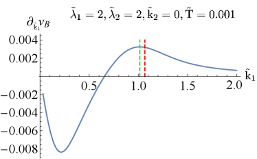
We also study the behavior of butterfly velocity $v_{B}$ along $x$ direction near the QPT. Fig. 5 shows $\partial_{\tilde{k}_{1}}v_{B}$ as the function of $\tilde{k}_{1}$ at $\tilde{T}=0.001$ with different $\tilde{k}_{2}$. We find that even when the lattice effect along $y$ direction is introduced, $v_{B}$ along $x$ direction can diagnose the QPT along $x$ direction. It indicates there is a rapid change of $v_{B}$ as well as the local extremes of $\partial_{k}v_{B}$ near the QCPs.

The essence of the above phenomenon is that the occurrence of quantum phase transition is usually accompanied by the change of IR fixed point. The power-law relationship between butterfly velocity and temperature at zero temperature limit is directly determined by IR fixed point. Therefore, the first derivative of the butterfly velocity with the system parameters will show an obvious peak behavior when it crosses the fixed point.

Notice that the butterfly velocity presents a discontinuity in the first-order derivative in the process of holographic superconductivity phase transition Ling:2016wuy . It is worth noting that the phenomena in quantum phase transition are different from this, and the mechanisms behind them are also completely different. The superconductivity phase transition will be accompanied by condensation, and the background geometry of the system will certainly be modified. From the perturbation analysis, it can be seen that the order of the perturbation received by the metric is twice that of the condensation field. Therefore, it can be concluded that the butterfly velocity in Ling:2016wuy has an obvious scaling law at the critical point, and its critical exponent is $1$. The MIT phase transition discussed in this paper is driven by the change of IR fixed point, and there is no emergence of the condensation. Therefore, the power-law dependence of butterfly velocity on temperature can well reflect this point.

Next, we want to study the behavior of $v_{B}$ in the zero-temperature limit.

In Ref. Blake:2016sud , they deduced that metallic phases in one-dimensional Q-lattice model always correspond to the well-known AdS${}_{2}\times\mathbb{R}^{2}$ IR geometry, on which $v_{B}\sim\tilde{T}^{1/2}$. And then, in our previous work Ling:2016ibq , we find that for the one-dimensional Q-lattice model, the scaling of $v_{B}$ with temperature is $v_{B}\sim\tilde{T}^{\alpha}$ in both metallic and insulating phases, but the exponent $\alpha$ approaches $1$ (in fact it is slightly larger than $1$) in insulating phase, which is different from that in metallic phase. It indicates the theory flows to different IR fixed points for metallic and insulating phases, respectively.

We also assume that in two-dimensional Q-lattice model the scaling of $v_{B}$ follows the same behavior as $v_{B}\sim\tilde{T}^{\alpha}$. In addition, we also assume $V_{xx}/V_{yy}\sim\tilde{T}^{\beta}$. Then, $\mathfrak{v}_{B}(\theta)$ becomes,

Therefore we have the temperature power exponent as

where $\prime$ denotes the derivative with respect to the temperature $\tilde{T}$. Explicitly, we can work out the temperature power exponent for some special $\theta$ as

Now, we begin to numerically study the behavior of $\mathfrak{v}_{B}$ in zero-temperature limit. And then we also try to understand the corresponding behavior based on the above assumption. Fig. 6 exhibits $\tilde{T}\mathfrak{v}^{\prime}_{B}/\mathfrak{v}_{B}$ as the function of $\tilde{T}$ for different phases over isotropy background. We clearly see that for metallic phases, $\alpha=1/2$. As expected it is the same as the metallic phase of the one-dimensional Q-lattice model. This suggests that the metallic phases for the isotropic 2-lattice system are essentially the same as that of the 1-lattice system. This is as expected since adding an extra copy in a perpendicular direction shall not change the IR geometry too much. However, for insulating phases, $\alpha$ approaches $1$ but is slightly smaller than $1$. It indicates that the insulating phase over isotropy two-dimensional Q-lattice model flows a novel IR fixed point, which is different from the well-known AdS${}_{2}\times\mathbb{R}^{2}$ IR geometry as expected, is also different from that of one-dimensional Q-lattice model where the $\alpha$ approaches a fixed value slightly larger than unity. Given the mild difference for insulating phases, the insulating phases indeed converge to certain fixed values.

Then we study the anisotropy two-dimensional Q-lattice model. The first case is that the system is a metallic phase in any direction. Fig. 7 shows $\tilde{T}\mathfrak{v}_{B}^{\prime}/\mathfrak{v}_{B}\,v.s.\,\tilde{T}$ over anisotropy background for $\tilde{k}_{1}=1.5$ and $\tilde{k}_{2}=1.5,\,1.2,\,1.1$, respectively. First, we see that for fixed lattice parameter, $\tilde{T}\mathfrak{v}_{B}^{\prime}/\mathfrak{v}_{B}$ tends to converge to a fixed value down to ultra-low temperature $\tilde{T}=10^{-7}$ for different angle $\theta$. This actually reflects the fact that $V_{xx}/V_{yy}$ is regular in zero-temperature limit when both directions are in metallic phase. The angular independence of the $\tilde{T}\mathfrak{v}_{B}^{\prime}/\mathfrak{v}_{B}$ means that $\lim_{T\to 0}\beta\to 0$, from Eq. (13) we find that the $\mathfrak{v}_{B}(\theta)$ converges to a fixed value along any direction. Secondly, for different lattice parameters, $\tilde{T}\mathfrak{v}_{B}^{\prime}/\mathfrak{v}_{B}$ tends to converge to a different value in the zero-temperature limit, which indicates that the theory flows to different IR fixed points. This is a key difference from the case with a single lattice, where the metallic phases are shown related only to the AdS${}_{2}\times\mathbb{R}^{2}$ IR fixed points.

However, when the anisotropy becomes larger (here, we take $\tilde{k}_{1}=1.5$ and $\tilde{k}_{2}=1$), we observe an novel phenomenon that, at least down to the $\tilde{T}\sim 10^{-9}$, $v_{B}$ does no longer follow the behavior $v_{B}\sim\tilde{T}^{\alpha}$ (see Fig. 8). Notice that this system is still metallic phase in any direction. On the other hand, we also observe that the $\tilde{T}v^{\prime}_{Bx}/v_{Bx}$ is smaller than that of $\tilde{T}v^{\prime}_{By}/v_{By}$, while the $\tilde{T}v^{\prime}_{B,\theta=\pi/4}/v_{B,\theta=\pi/4}$ converges to that of $\tilde{T}v^{\prime}_{Bx}/v_{Bx}$. This suggests that in the limit of zero temperature, $\beta$ does not tend to vanishing and we conclude that $\beta>0$.

Another anisotropic case is that the system is in metallic phase in $x$ direction and insulating phase in $y$ direction. The behaviors for this case are shown in Fig. 9. We see that along $x$ direction, $\tilde{T}\mathfrak{v}_{B}^{\prime}/\mathfrak{v}_{B}$ converges to a fixed value being smaller than unity. While along $y$ direction, $\tilde{T}\mathfrak{v}_{B}^{\prime}/\mathfrak{v}_{B}$ converges to a fixed value being larger than unity. Notice that, the $\tilde{T}\mathfrak{v}^{\prime}_{Bx}/\mathfrak{v}_{Bx}$ is smaller than that of $\tilde{T}\mathfrak{v}^{\prime}_{By}/\mathfrak{v}_{By}$, while the $\tilde{T}\mathfrak{v}^{\prime}_{B,\theta=\pi/4}/\mathfrak{v}_{B,\theta=\pi/4}$ seems converge to that of $\tilde{T}\mathfrak{v}^{\prime}_{By}/\mathfrak{v}_{By}$. This situation is delicate, since $\tilde{T}\mathfrak{v}^{\prime}_{Bx}/\mathfrak{v}_{Bx}<\mathfrak{v}^{\prime}_{By}/\mathfrak{v}_{By}$ suggests $\beta>0$, while $\tilde{T}\mathfrak{v}^{\prime}_{B,\theta=\pi/4}/\mathfrak{v}_{B,\theta=\pi/4}$ converging to $\tilde{T}\mathfrak{v}^{\prime}_{Bx}/\mathfrak{v}_{Bx}$ suggests $\beta<0$. This seemingly contradicted conclusion is on account of the temperature so far is not low enough. Closer examination of the zoom in inset in Fig. 9 will reveal that, $\tilde{T}\mathfrak{v}^{\prime}_{B,\theta=\pi/4}/\mathfrak{v}_{B,\theta=\pi/4}$ starts to deviate from $\tilde{T}\mathfrak{v}^{\prime}_{By}/\mathfrak{v}_{By}$, and it will converge to $\tilde{T}\mathfrak{v}^{\prime}_{Bx}/\mathfrak{v}_{Bx}$ in even lower temperature. In this case, we still have that $\beta>0$.

Next, we elaborate on the anisotropic case where the system is insulating phase in any direction (Fig. 10). $\tilde{T}\mathfrak{v}_{B}^{\prime}/\mathfrak{v}_{B}$ converges to different fixed value equaling to or being smaller than unity for different angle $\theta$. The $\tilde{T}\mathfrak{v}^{\prime}_{Bx}/\mathfrak{v}_{Bx}$ and $\tilde{T}\mathfrak{v}^{\prime}_{By}/\mathfrak{v}_{By}$ converge to slightly different values, while $\tilde{T}\mathfrak{v}^{\prime}_{B,\theta=\pi/4}/\mathfrak{v}_{B,\theta=\pi/4}$ converges to that of $\tilde{T}\mathfrak{v}^{\prime}_{By}/\mathfrak{v}_{By}$. This means that $V_{xx}/V_{yy}\sim\tilde{T}^{\beta}$ with $\beta<0$, i.e., the $\lim_{T\to 0}V_{xx}/V_{yy}\to\infty$. This is different from the case where the system is in the metallic phase in any direction.

Before closing this subsection, we would like to give some comments. First, according to the properties of the DC conductivity with the temperature, the anisotropic system can be categorized into three classes:

• •

  Case 1: The system is in the metallic phase in any direction.

• •

  Case 2: The system is in the metallic phase in $x$ direction and insulating phase in $y$ direction.

• •

  Case 3: The system is in the insulating phase in any direction.

Further, by using the scaling behavior of the butterfly, we can meticulously depict this anisotropic system by the parameter $\beta$.

• •

  When the system is in the metallic phase in any direction (case 1), $\beta=0$ for mildly anisotropic lattice.

• •

  When further increasing the anisotropy, $\beta>0$. This phenomenon persists from case 1 to case 2.

• •

  When the system is insulating phase in any direction, $\beta<0$.

To summarize, for anisotropic cases, the most important property is that the IR fixed point can be non-AdS${}_{2}\times\mathbb{R}^{2}$ even for metallic phases. Also, we observed some patterns of $\alpha$ and $\beta$ for different cases. This may help explain the bizarre IR fixed point. In addition, the above phenomena show that in most cases, there is indeed a scaling relationship between butterfly velocity and temperature. Moreover, the scaling relationship of butterfly velocity along different directions is indeed consistent with the deduced relationship Eq. (14). This shows that the above numerical results do verify the hypothesis given in Eq. (12) and Eq. (14).

References

- (1) Glotzer, Sharon C., and Michael J. Solomon. “Anisotropy of building blocks and their assembly into complex structures.” Nature materials 6.8 (2007): 557.
- (2) J. M. Maldacena, “The Large N limit of superconformal field theories and supergravity,” Adv. Theor. Math. Phys. 2, 231 (1998) [hep-th/9711200].
- (3) S. S. Gubser, I. R. Klebanov and A. M. Polyakov, “Gauge theory correlators from noncritical string theory,” Phys. Lett. B 428, 105 (1998) [hep-th/9802109].
- (4) E. Witten, “Anti-de Sitter space and holography,” Adv. Theor. Math. Phys. 2, 253 (1998) [hep-th/9802150].
- (5) O. Aharony, S. S. Gubser, J. M. Maldacena, H. Ooguri and Y. Oz, “Large N field theories, string theory and gravity,” Phys. Rept. 323, 183 (2000) [hep-th/9905111].
- (6) S. A. Hartnoll, A. Lucas and S. Sachdev, “Holographic quantum matter,” arXiv:1612.07324 [hep-th].
- (7) Y. Ling, “Holographic lattices and metal-insulator transition,” Int. J. Mod. Phys. A 30 (2015) no.28&29, 1545013.
- (8) L. Q. Fang, X. H. Ge, J. P. Wu and H. Q. Leng, “Anisotropic Fermi surface from holography,” Phys. Rev. D 91, no. 12, 126009 (2015) [arXiv:1409.6062 [hep-th]].
- (9) I. Aref’eva and K. Rannu, “Holographic Anisotropic Background with Confinement-Deconfinement Phase Transition,” JHEP 1805, 206 (2018) [arXiv:1802.05652 [hep-th]].
- (10) H. S. Jeong, Y. Ahn, D. Ahn, C. Niu, W. J. Li and K. Y. Kim, “Thermal diffusivity and butterfly velocity in anisotropic Q-Lattice models,” JHEP 1801, 140 (2018) [arXiv:1708.08822 [hep-th]].
- (11) S. Cremonini, X. Dong, J. Rong and K. Sun, “Holographic RG flows with nematic IR phases,” JHEP 07 (2015), 082 [arXiv:1412.8638 [hep-th]].
- (12) N. Grandi, V. Juričić, I. Salazar Landea and R. Soto-Garrido, “Towards holographic flat bands,” JHEP 05 (2021), 123 [arXiv:2103.01690 [hep-th]].
- (13) M. Baggioli, V. C. Castillo and O. Pujolas, “Black Rubber and the Non-linear Elastic Response of Scale Invariant Solids,” JHEP 09 (2020), 013 [arXiv:2006.10774 [hep-th]].
- (14) A. Donos and J. P. Gauntlett, ”Holographic charge density waves,” Phys. Rev. D 87, no. 12, 126008 (2013) doi:10.1103/PhysRevD.87.126008 [arXiv:1303.4398 [hep-th]].
- (15) Y. Ling, C. Niu, J. Wu, Z. Xian and H. b. Zhang, ”Metal-insulator Transition by Holographic Charge Density Waves,” Phys. Rev. Lett. 113, 091602 (2014) [arXiv:1404.0777 [hep-th]].
- (16) A. Donos and J. P. Gauntlett, “Novel metals and insulators from holography,” JHEP 1406, 007 (2014) [arXiv:1401.5077 [hep-th]].
- (17) M. Blake and A. Donos, “Quantum Critical Transport and the Hall Angle,” Phys. Rev. Lett. 114, no. 2, 021601 (2015) [arXiv:1406.1659 [hep-th]].
- (18) A. Donos and J. P. Gauntlett, “Thermoelectric DC conductivities from black hole horizons,” JHEP 1411, 081 (2014) [arXiv:1406.4742 [hep-th]].
- (19) Z. Zhou, J. P. Wu and Y. Ling, “DC and Hall conductivity in holographic massive Einstein-Maxwell-Dilaton gravity,” JHEP 1508, 067 (2015) [arXiv:1504.00535 [hep-th]].
- (20) A. Donos, B. Goutŕaux and E. Kiritsis, “Holographic Metals and Insulators with Helical Symmetry,” JHEP 1409, 038 (2014) [arXiv:1406.6351 [hep-th]].
- (21) Y. Ling, P. Liu, J. P. Wu and Z. Zhou, “Holographic Metal-Insulator Transition in Higher Derivative Gravity,” Phys. Lett. B 766, 41 (2017) [arXiv:1606.07866 [hep-th]].
- (22) J. P. Wu, “Transport phenomena and Weyl correction in effective holographic theory of momentum dissipation,” Eur. Phys. J. C 78, no. 4, 292 (2018) [arXiv:1902.03225 [hep-th]].
- (23) Y. Ling, P. Liu, C. Niu, J. P. Wu and Z. Y. Xian, “Holographic Entanglement Entropy Close to Quantum Phase Transitions,” JHEP 1604, 114 (2016) [arXiv:1502.03661 [hep-th]].
- (24) Y. Ling, P. Liu, C. Niu and J. P. Wu, “Building a doped Mott system by holography,” Phys. Rev. D 92, no. 8, 086003 (2015) [arXiv:1507.02514 [hep-th]].
- (25) Y. Ling, P. Liu and J. P. Wu, ”A novel insulator by holographic Q-lattices,” JHEP 1602, 075 (2016) [arXiv:1510.05456 [hep-th]].
- (26) Y. Ling, P. Liu and J. P. Wu, “Characterization of Quantum Phase Transition using Holographic Entanglement Entropy,” Phys. Rev. D 93, no. 12, 126004 (2016) [arXiv:1604.04857 [hep-th]].
- (27) Y. Ling, P. Liu and J. P. Wu, “Holographic Butterfly Effect at Quantum Critical Points,” JHEP 1710, 025 (2017) [arXiv:1610.02669 [hep-th]].
- (28) M. Baggioli and O. Pujolas, “Electron-Phonon Interactions, Metal-Insulator Transitions, and Holographic Massive Gravity,” Phys. Rev. Lett. 114, no. 25, 251602 (2015) [arXiv:1411.1003 [hep-th]].
- (29) M. Baggioli and O. Pujolas, “On holographic disorder-driven metal-insulator transitions,” JHEP 1701, 040 (2017) [arXiv:1601.07897 [hep-th]].
- (30) M. Baggioli and O. Pujolas, “On Effective Holographic Mott Insulators,” JHEP 1612, 107 (2016) [arXiv:1604.08915 [hep-th]].
- (31) Y. S. An, T. Ji and L. Li, “Magnetotransport and Complexity of Holographic Metal-Insulator Transitions,” JHEP 10 (2020), 023 [arXiv:2007.13918 [hep-th]].
- (32) D. A. Roberts and B. Swingle, “Lieb-Robinson Bound and the Butterfly Effect in Quantum Field Theories,” Phys. Rev. Lett. 117, no. 9, 091602 (2016) [arXiv:1603.09298 [hep-th]].
- (33) S. H. Shenker and D. Stanford, “Black holes and the butterfly effect,” JHEP 1403, 067 (2014) [arXiv:1306.0622 [hep-th]].
- (34) S. H. Shenker and D. Stanford, “Multiple Shocks,” JHEP 1412, 046 (2014) [arXiv:1312.3296 [hep-th]].
- (35) S. H. Shenker and D. Stanford, “Stringy effects in scrambling,” JHEP 1505, 132 (2015) [arXiv:1412.6087 [hep-th]].
- (36) M. Blake, “Universal Charge Diffusion and the Butterfly Effect in Holographic Theories,” Phys. Rev. Lett. 117, no. 9, 091601 (2016) [arXiv:1603.08510 [hep-th]].
- (37) J. Maldacena, S. H. Shenker and D. Stanford, “A bound on chaos,” JHEP 1608, 106 (2016) [arXiv:1503.01409 [hep-th]].
- (38) M. Blake, “Universal Diffusion in Incoherent Black Holes,” Phys. Rev. D 94, no. 8, 086014 (2016) [arXiv:1604.01754 [hep-th]].
- (39) A. Lucas and J. Steinberg, “Charge diffusion and the butterfly effect in striped holographic matter,” JHEP 1610, 143 (2016) [arXiv:1608.03286 [hep-th]].
- (40) S. A. Hartnoll, “Theory of universal incoherent metallic transport,” Nature Phys. 11, 54 (2015) [arXiv:1405.3651 [cond-mat.str-el]].
- (41) Y. Ling, P. Liu and J. P. Wu, “Note on the butterfly effect in holographic superconductor models,” Phys. Lett. B 768, 288 (2017) [arXiv:1610.07146 [hep-th]].
- (42) M. Baggioli, B. Padhi, P. W. Phillips and C. Setty, “Conjecture on the Butterfly Velocity across a Quantum Phase Transition,” JHEP 07 (2018), 049 [arXiv:1805.01470 [hep-th]].
- (43) A. Donos and J. P. Gauntlett, “Holographic Q-lattices,” JHEP 1404, 040 (2014) [arXiv:1311.3292 [hep-th]].
- (44) Y. Ling, P. Liu, C. Niu, J. P. Wu and Z. Y. Xian, “Holographic Superconductor on Q-lattice,” JHEP 1502, 059 (2015) [arXiv:1410.6761 [hep-th]].
- (45) A. Hosseini, H. Nejati and Y. Massoud, “A Metal-Insulator-Metal based two-dimensional triangular lattice photonic band-gap structure,” 2007 50th Midwest Symposium on Circuits and Systems, 2007, pp. 1253-1256, doi: 10.1109/MWSCAS.2007.4488780.
- (46) J. Zaanen, Superconductivity: Why the temperature is high, Nature 430 (2004) 512.
- (47) S. Sachdev and B. Keimer, “Quantum Criticality,” Phys. Today 64N2 (2011), 29 [arXiv:1102.4628 [cond-mat.str-el]].
- (48) K. Y. Kim and C. Niu, “Diffusion and Butterfly Velocity at Finite Density,” JHEP 06 (2017), 030 [arXiv:1704.00947 [hep-th]].