Dynamic generation of nonequilibrium superconducting states in Kitaev chain
Abstract
A non-equilibrium state shares macroscopic properties, such as conductivity and superconductivity, with a static state when the two states exhibit an identical average value of an observable over a period. We studied the quench dynamics of a Kitaev chain on the basis of two types of order parameters associated with two channels of pairing: local pairing in real space and Bardeen-Cooper-Schrieffer (BCS)-like pairing in momentum space. On the basis of the exact solution, we found that the two order parameters were identical for the ground state, which indicated a balance between the two pairing channels and would help determine the quantum phase diagram. However, for a non-equilibrium state obtained through time evolution from an initially prepared vacuum state, the two parameters varied; however, both parameters could still help determine the phase diagram. In the region of nontrivial topological phases, non-equilibrium states favored BCS-like pairing. This paper presents an alternative approach to dynamically generate a superconducting state from a trivial empty state and illuminates the pairing mechanism.
I Introduction
The topic of non-equilibrium phenomena in quantum many-body systems is fundamental and compelling in condensed matter physics. In conventional theory, quantum phase transitions occur at zero temperature, and a phase diagram refers, in particular, to the ground state of a system. However, it is obviously that the ground state is intimately related to the excited states for a certain class of systems since they all stem from a same time-independent Hamiltonian. For instance, for a Hamiltonian written in pseudospin form , the ground state is determined by the field distribution ZG , which can be extracted from any eigenstates in the tensor product form. In this sense, non-equilibrium phenomena within the prethermalization regime can probably reflect the phase diagram from an alternative aspect. A well-known probe of many-body quantum dynamics is quantum quench, in which a many-body system is initially prepared in a state that is typically the ground state of some simple Hamiltonian and subsequently evolves with a different Hamiltonian. In a conventional framework, the properties of prequench and postquench Hamiltonians are extracted from the evolved states instead of the ground state. The use of nonequilibrium many-body dynamics presents an alternative approach for accessing a new exotic quantum state with an energy level considerably different from that of the ground state Choi ; Else ; Khemani ; Lindner ; Kaneko ; Tindall ; YXMPRA ; ZXZPRB2 ; TK ; JT1 ; JT2 . Advancements in atomic physics, quantum optics, and nanoscience have allowed the development of artificial systems with high accuracy Jochim ; Greiner . Thus, theoretical models can be simulated and realized experimentally. Direct simulation of a simple model is useful not only for solving key challenges in condensed matter physics but also in the engineering design of quantum devices. Notably, the availability of an experimentally controllable fermion system provides an unprecedented opportunity to explore nonequilibrium dynamics in interacting many-body systems.
In addition, it has recently been established that experiments with various materials and excitation conditions have witnessed phenomena with no equilibrium analog or accessibility of chemical substitution, including superconducting-like phases AC ; DF ; MM ; TS , charge density waves (CDW) LS ; HM ; AK and excitonic condensation YM . Therefore, how to stabilize a system in a non-equilibrium superconducting phase with a long lifetime is a great challenge and is at the forefront of current research. Among various non-equilibrium protocols, the generation of the -pairing-like state plays a pivotal role in which the existence of doublon and holes facilitate the superconductivity SK ; TK ; JT ; FP ; RF1 ; RF2 ; SE ; JL ; TK2 ; ZXZPRB2 ; ZXZPRB3 ; JT1 ; JT2 .
In the present paper, we report our theoretical investigation of nonequilibrium dynamics in a paradigmatic quantum many-body model—the Kitaev chain. Comparing to the previous works on the Hubbard model, the intial state is an easily prepared state YXMPRA and quenched Hamiltonian is time-independent with parameters covering rich phase diagram in the present work. The Kitaev chain is a lattice model of a p-wave superconducting wire, which realizes Majorana zero modes at the ends of the chain Kitaev . Unpaired Majorana modes have been exponentially localized at the ends of open Kitaev chains Sarma ; Stern ; Alicea . The primary feature of this model originates from the pairing term, which violates the conservation of the fermion number but preserves its parity, leading to a superconducting state. In general, most studies on this model have centered on the ground state or the dynamical quantum phase transitions related to the ground state MH ; LZ . The strength of the pairing interactions has an important role in giving rise to a gapped superconducting state. However, knowledge regarding the pair in each quantum phase remains limited. Specifically, the nearest-neighbor (NN) pair creation (annihilation) term is subtle for the formation of a pair. It results in an NN pair in real space. By contrast, the Hamiltonian in k-space indicates that it also contributes to Bardeen-Cooper-Schrieffer (BCS)-like pairing in momentum space, which involves two particles with opposite momentum. In addition, distinct features originate from the pair term in not only statics but also dynamics. To determine the features of a given state, we introduced two types of order parameters associated with two channels of pairing: local pairing in real space and BCS-like pairing in momentum space. On the basis of the exact solution, we found that the two order parameters were identical for the ground state and could help determine the quantum phase diagram. This revealed an unprecedented feature of the ground state that helps balance between two types of pairing channels. The primary aim of this study was to obtain pertinent information regarding the nonequilibrium state. In this study, acquisition of a vacuum state by the quench process, in which a prequench Hamiltonian has infinite chemical potential, was considered to be the ground state. We investigated evolved states under the postquench Hamiltonian with parameters covering the entire region and found two types of order parameters that were different but could help determine the quantum phase diagram. Our results yield two key findings: a superconducting state can be dynamically generated from a trivial state, and the difference between two types of order parameters for a nonequilibrium state indicates the generation of various superconducting states from the ground state, thus expanding the variety of the state of matter that is associated with different channels of pairing.
This paper is organized as follows. In Sec. II, we present the model and introduce two types of order parameters to investigate the feature of superconducting state. In Subsecs. II.1 and II.2, we calculate the order parameters in space and real space for the ground state, respectively. In Sec. III, we investigate the features of dynamic behavior of the system. Finally, we give a summary and discussion in Section IV. Some details of the derivations are given in Appendix.


II Model and order parameters
We consider the following fermionic Hamiltonian on a lattice of length
| (1) | |||||
where is a fermionic creation (annihilation) operator on site , , the tunneling rate, the chemical potential, and the strength of the -wave pair creation (annihilation). is defined for periodic boundary condition. The Hamiltonian in Eq. (1) has a rich phase diagram that describes a spin-polarized -wave superconductor in one dimension. This system has a topological phase in which a zero- energy Majorana mode is located at each end of a long chain. It is the fermionized version of the well-known one-dimensional transverse-field Ising model Pfeuty , which is one of the simplest solvable models that exhibits quantum criticality and phase transition with spontaneous symmetry breaking SachdevBook .Several studies have been conducted with a focus on long-range Kitaev chains, in which the superconducting pairing term decays with distance as a power law TPCHOY ; AGG ; DV1 ; DV2 ; OV ; LL ; UB .
This study centered on the dynamics of a system with NN superconducting pairing term, which warrants further-systematic studies, such as those on long-range correlations. The Hamiltonian can be exactly solved based on Fourier transformation (see Appendix A). The ground-state wave function can be expressed as
| (2) |
with groundstate energy
| (3) |
Accordingly, the phase diagram can be obtained from and , with the phase boundaries
| (4) |
These lines separate four regions in the parameter space, representing different phases with winding numbers CKC ; NL , and , respectively. Fig. 1(a) depicts the phase diagram. The phase diagram indicates that the chemical potential has a subtle role in the ground state. It restricts the value of to maintain the non-trivial phases. The might be because the sufficiently large suppresses pair creation. Thus the number of pairs is higher in nontrivial phases than in trivial phases which leads to the following two questions. First, how to quantify the amount of pairs in each phase? Second, what are the features of the pairing in real or momentum space. The answers are the main part of our goals in this work.
To answer the questions, we explore the features of a superconducting state by introducing two types of order parameters BP . Two operators and characterize pairing channels in real space with
| (5) |
and space with
| (6) |
For a given state , the quantity helps measure the rate of transition for a pair located around the th site, whereas helps measure the rate of transition for a pair at the channel. The corresponding order parameters are defined on the basis of the average magnitude over all channels, as expressed in
| (7) |
and
| (8) |
Nonzero and indicate that the state is a superconducting state. In general, and have different values for a given state. In the following subsections, we describe the analytical expressions of and for the ground states of the system in different regions and their behaviors at phase boundaries.
II.1 Pairing in space
The order parameter of the ground state is expressed as
| (9) |
Direct derivation shows that the order parameter is
| (10) |
in the large limit, which can be expressed explicitly in the following regions. (i) When , the order parameter is
| (11) |
for but at . (ii) When , the order parameter is
| (12) |
for but at . This suggests that when is not dependent on . Unexpectedly, the number of pairs is determined using only the parameter in non-trivial phases. The underlying mechanism is an open question in this work. By contrast, when , decays as increases. Specifically, it decays linearly with for small and as for large .
Nevertheless, we can only understand this result mathematically from an example in classical Electromagnetics. We consider a charged conducting ellipsoid with the surface equations
| (13) |
The total charge is . Then surface charge density distribution along the axis is
| (14) |
And the electric potential at the origin is
| (15) |
where
| (16) |
Regardless of the integration, the physics tells us that is always constant when the origin lies inside the ellipsoid (). We note that the expression of is identical to the Eq. (10).
II.2 Pairing in real space
The following order parameter
| (17) |
is identical to . The fact that indicates that
| (18) |
Applying Fourier transformation in Eq. (A1) in the large limit, the following equation can be obtained:
| (19) |
This is the primary finding of the present study. It appears that the ground state favors a balance between the two types of pairing. However, not all states can maintain such a balance. Thus, the aformentioned queries are resolved. Regarding the first query, two types of order parameters are deliberately selected to quantify the number of pairs in two aspects. Regarding the second query, the equality of the two quantities and for the ground state itself is a key feature of the ground state.
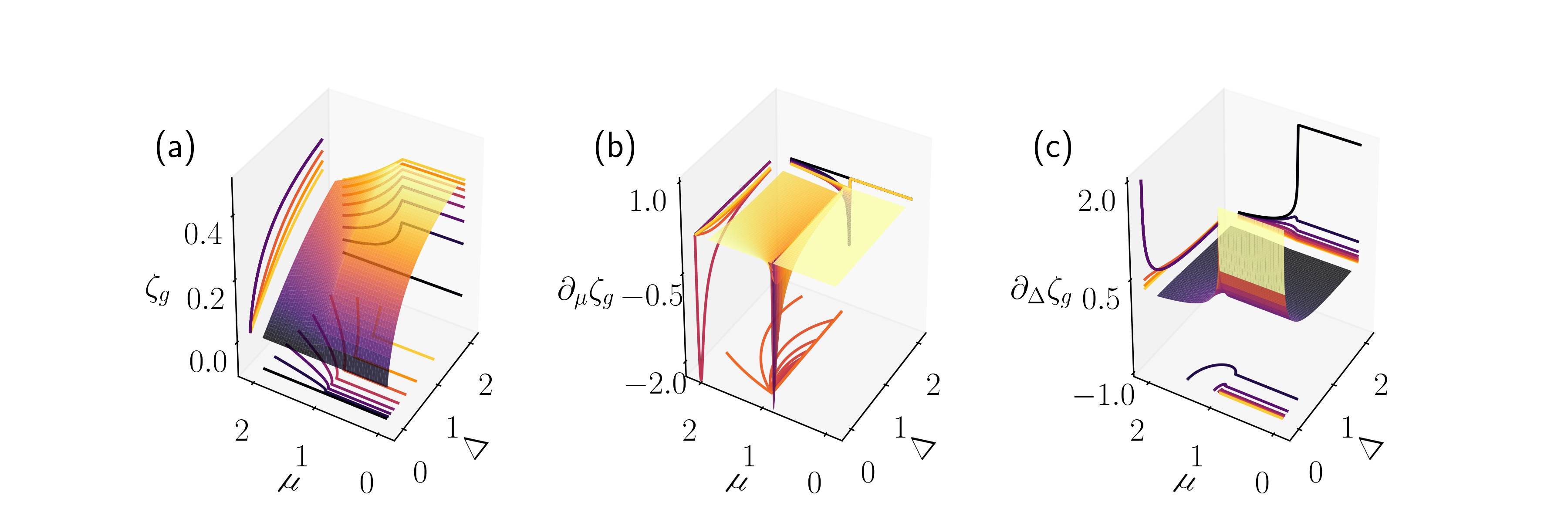
In particular, the analytical behavior of () as function of can identify the phase diagram (see Appendix B). It is found that second-order quantum phase transitions occur at phase boundaries. The first-order derivatives of two parameters with respect to or are discontinuous, and then result in the divergence of the corresponding second-order derivatives. The profiles of at the line and are presented in Figs. 1(b) and 1(c), respectively. and its partial derivatives with respect to and for a finite lattice in the first quadrant of the plane are shown in Figs. 2(a)-2(c). Numerical data for the finite system reveal that the divergence at phase boundaries is demonstrated by peaks.
III Non-equilibrium stationary state
In this section, we present the features of the dynamic behavior of the system. It relates to the time evolution for a particular initial state
| (20) |
which is essentially an empty state for fermion in real space. The evolved state
| (21) | |||||
may trend toward a stationary state after a sufficiently long time. The non-equilibrium stationary state driven by is intimately associated with the phase diagram of the ground state (Fig. 1(a)). We focus on the time-dependent order parameters for the evolved state . Based on the fact that represents the eigenstates of the operator , the following explicit forms can be obtained:
| (22) | |||||
and
| (23) | |||||
where the key function is
| (24) |
Figs. 3(b1) and 3(b2) present and as the function of time for finite-size systems with several typical system parameters . As expected, both quantities become steady after a long period. and behave as damping oscillations around a certain equilibrium position. The quasi frequencies and decay rates can be evaluated through a saddle point integration in the continuum limit AS ; AAM ; SA . We rewrite in the form
| (25) |
where
| (26) | |||||
| (27) |
The results depends on the location of the extrema . (i) In this case with , we have quasi frequency and . (ii) In this case with , we have quasi frequency and . Similar analysis can be applied to . These results accord with the plots in Fig. 4.
On the other hand, such behaviors can also be understood by a simple picture, when the spectrum contains higher degeneracy, which relates to the peak of the density of state (DOS) of the system. The DOS at energy level is generally defined as
| (28) |
where d indicates the number of energy levels that appear in the interval with the normalization factor . Figs. 3(c1)-3(c4), depict the energy levels and DOS as the functions of momentum and , respectively. When the peaks of appear, the quasi frequency is related to the energy band gap , which is the distance between two peaks.
No matter what mechanism of the decay, and approach to their stable values, which can be obtained from
| (29) |
and
| (30) |
It is two types of summation for the same function . In the large limit, and can be expressed as the integral equations:
| (31) |
and
| (32) |
Straightforward derivations lead to the development of analytical expressions
| (33) |
where at , and
| (34) | |||||
when . Conversely,
| (35) |
the time-averaged analytical expressions for and obtained from Eqs. (33) and (35) are shown graphically in Fig. 3(a).
Similar to the static order parameters, analytical behavior of and as function of can still identify the phase diagram (see Appendix B). Fig. 5 shows the average order parameters and obtained from Eqs. (29) and (30) as the function of and for the case in the first quadrant of the plane. Fig. 6 presents , and , the partial dervatives of and with respect to and , for finite system. Fig. 7(a1)-7(a3) show the profiles of , , and at the line Fig. 7(b1)-7(b3) present the profiles of , , and at the line , indicating that four quantities, , and , can identify the phase boundary at and . Compared with and which are always identical in all regions, and vary in non-trivial regions, providing quantitative description of the pairing mechanism for a non-equilibrium state. Moreover, the non-equilibrium state is also a superconducting state because the values of and have the same order as those of and . The fact that indicates that BCS-like pairing in momentum space is favored. Before ending this work, we would like to point out that the obtained results depend on the initial state. For example, consider an initial state in the form
| (36) |
with , which is the eigenstate of with arbitrary parameters due to the fact
| (37) |
from the Appendix A. We find that
| (38) |
which result in , indicating that quantities and cannot indicate the phase diagram.
IV Summary
In summary, we have studied the quench dynamics of a Kitaev chain by introducing two types of order parameters that characterize two different pairing mechanisms, namely local pairing in real space and BCS-like pairing in momentum space. We have shown exactly that the ground states over the entire parameter region support the identical values of them, indicating a balance between the two types of pairing channels; This is an unprecedented feature of the ground state. The balance is disturbed in a non-equilibrium state when the post-quench Hamiltonian is in a topologically non-trivial phase, whereas it is maintained in a topologically trivial phase. Furthermore, non-equilibrium superconducting states favor the BCS-like pairing. —Our findings present an alternative approach to generate a superconducting state from a trivial empty state and illuminate the pairing mechanism.
Acknowledgment
We acknowledge the support of NSFC (Grants No. 11874225).
Appendix A Solution and phase diagram
The Hamiltonian (1) is exactly solvable because of the translational symmetry of the system, i.e., , where is the translational operator, which is defined by . Taking the Fourier transformation
| (A1) |
of the Hamiltonian (1), with wave vector , we can obtain the following equation:
| (A2) | |||||
For ease of further analysis, the value can be considered to be and the Hamiltonian can be expressed through the Nambu representation
| (A3) | |||||
| (A9) |
where the Hamiltonian in each invariant subspace satisfies the commutation relation
| (A10) |
This allows us to treat the diagonalization and dynamics governed by individually. For a given , the Hamiltonian in the basis () is expressed as a matrix
| (A11) |
where and . The eigenstates [ denotes the even (odd) parity of the particle number] are
| (A12) | |||||
| (A13) |
where is the normalization coefficient in the context of Dirac inner product with
| (A14) |
and corresponding energies are
| (A15) |
with
| (A16) |
Accordingly, the ground-state wave function can be expressed as
| (A17) |
is the eigenstate of , obeying , where is a real number. Furthermore, the phase-transition lines (phase boundary) can be determined using min, which results in the gapless lines
| (A18) |
These lines separate four regions in the parameter space, representing different phases with winding numbers CKC ; NL , and , respectively.
Appendix B Analytical behavior of static and dynamic order parameters
The analytical behavior of () as the function of can identify the phase diagram. On the basis of the aforementioned euqations, we found that second-order quantum phase transitions occur at phase boundaries. Around lines , we have at but at . Then, diverges at these two lines. We have
| (B 1) | |||||
| (B 2) | |||||
| (B 3) |
around the segment .
Similarly, the analytic expressions of and help us investigate their analytical behaviors. (i) Around lines , we have
| (B 4) |
which is divergent at the phase boundary . By contrast, when we have
| (B 5) |
which is divergent. However, we have at . Therefore, is discontinuous at the lines . (ii) Around the segment (), we have
| (B 6) |
for , resulting in the divergent . By contrast, we have
| (B 7) |
for . It is divergent at the phase boundary . In summary, , and , can identify the phase boundary at and . Compared with and which are always identical in all regions, and vary in non-trivial regions, providing quantitative description of the pairing mechanism for a non-equilibrium state. Moreover, the non-equilibrium state is also a superconducting state because the values of and have the same order as those of and . The fact that indicates that BCS-like pairing in momentum space is favored.
References
- (1) G. Zhang and Z. Song, Topological Characterization of Extended Quantum Ising Models, Phys. Rev. Lett. 115, 177204 (2015).
- (2) S. Choi, J. Choi, R. Landig, G. Kucsko, H. Zhou, J. Isoya, F. Jelezko, S. Onoda, H. Sumiya, V. Khemani, C. v. Keyserlingk, N. Y. Yao, E. Demler, and M. D. Lukin, Observation of discrete time-crystalline order in a disordered dipolar many-body system, Nature 543, 221 (2017).
- (3) D. V. Else, B. Bauer, and C. Nayak, Floquet time crystals, Phys. Rev. Lett. 117, 090402 (2016).
- (4) V. Khemani, A. Lazarides, R. Moessner, and S. L. Sondhi, Phase structure of driven quantum systems, Phys. Rev. Lett. 116, 250401 (2016).
- (5) N. H. Lindner, G. Refael, and V. Galitski, Floquet Topological Insulator in Semiconductor Quantum Wells, Nat. Phys. 7, 490 (2011).
- (6) T. Kaneko, T. Shirakawa, S. Sorella, and S. Yunoki, Photoinduced Pairing in the Hubbard Model, Phys. Rev. Lett. 122, 077002 (2019).
- (7) J. Tindall, B. Buča, J. R. Coulthard, and D. Jaksch, Heating-Induced Long-Range Pairing in the Hubbard Model, Phys. Rev. Lett. 123, 030603 (2019).
- (8) X. M. Yang and Z. Song, Resonant generation of a p-wave Cooper pair in a non-Hermitian Kitaev chain at the exceptional point, Phys. Rev. A 102, 022219 (2020).
- (9) X. Z. Zhang and Z. Song, -pairing ground states in the non-Hermitian Hubbard model, Phys. Rev. B 103, 235153 (2021).
- (10) T. Kaneko, T. Shirakawa, S. Sorella, and S. Yunoki, Photoinduced Pairing in the Hubbard Model, Phys. Rev. Lett. 122, 077002 (2019).
- (11) J. Tindall, F. Schlawin, M. A. Sentef, and D. Jaksch, Analytical solution for the steady states of the driven Hubbard model, Phys. Rev. B 103, 035146
- (12) J. Tindall, F. Schlawin, M. Sentef and D. Jaksch, Lieb’s Theorem and Maximum Entropy Condensates, Quantum 5, 610 (2021).
- (13) S. Jochim, M. Bartenstein, A. Altmeyer, G. Hendl, S. Riedl, C. Chin, J. Hecker Denschlag, and R. Grimm, Bose-Einstein Condensation of Molecules, Science 302, 2101 (2003).
- (14) M. Greiner, C. A. Regal, and D. S. Jin, Emergence of a molecular Bose–Einstein condensate from a Fermi gas, Nature (London) 426, 537 (2003).
- (15) A. Cavalleri, Photo-induced superconductivity, Contemporary Physics, 59, 31 (2018).
- (16) D. Fausti, R. I. Tobey, N. Dean, S. Kaiser, A. Dienst, M. C. Ho mann, S. Pyon, T. Takayama, H. Takagi, and A. Cavalleri, Light-Induced Superconductivity in a Stripe-Ordered Cuprate, Science 331, 189 (2011).
- (17) M. Mitrano, A. Cantaluppi, D. Nicoletti, S. Kaiser, A. Perucchi, S. Lupi, P. Di Pietro, D. Pontiroli, M. Ricc, S. R. Clark, et al., Nature 530, 461 (2016).
- (18) T. Suzuki, T. Someya, T. Hashimoto, S. Michimae, M. Watanabe, M. Fujisawa, T. Kanai, N. Ishii, J. Itatani, S. Kasahara, et al., Photoinduced possible superconducting state with long-lived disproportionate band filling in FeSe, Commun. Phys. 2, 115 (2019).
- (19) L. Stojchevska, I. Vaskivskyi, T. Mertelj, P. Kusar, D. Svetin, S. Brazovskii, and D. Mihailovic, Science 344, 177 (2014).
- (20) H. Matsuzaki, M. Iwata, T. Miyamoto, T. Terashige, K. Iwano, S. Takaishi, M. Takamura, S. Kumagai, M. Yamashita, R. Takahashi, et al., Excitation-Photon-Energy Selectivity of Photoconversions in Halogen-Bridged Pd-Chain Compounds: Mott Insulator to Metal or Charge-Density-Wave State, Phys. Rev. Lett. 113, 096403 (2014).
- (21) A. Kogar, A. Zong, P. E. Dolgirev, X. Shen, J. Straquadine, Y.-Q. Bie, X. Wang, T. Rohwer, I.-C. Tung, Y. Yang, et al., Light-induced charge density wave in LaTe3, Nat. Phys. 16, 159 (2020).
- (22) Y. Murotani, C. Kim, H. Akiyama, L. N. Pfei er, K. W. West, and R. Shimano, Light-driven electron-hole Bardeen-Cooper-Schrieffer-like state in bulk GaAs, Phys. Rev. Lett. 123, 197401 (2019).
- (23) S. Kitamura and H. Aoki, Phys. Rev. B 94, 174503 (2016).
- (24) J. Tindall, B. Bu ca, J. R. Coulthard, and D. Jaksch, Phys. Rev. Lett. 123, 030603 (2019).
- (25) R. Fujiuchi, T. Kaneko, Y. Ohta, and S. Yunoki, Phys. Rev. B 100, 045121 (2019).
- (26) F. Peronaci, O. Parcollet, and M. Schir o, Phys. Rev. B 101, 161101 (2020).
- (27) R. Fujiuchi, T. Kaneko, K. Sugimoto, S. Yunoki, and Y. Ohta, Phys. Rev. B 101, 235122 (2020).
- (28) S. Ejima, T. Kaneko, F. Lange, S. Yunoki, and H. Fehske, Phys. Rev. Research 2, 032008 (2020).
- (29) J. Li, D. Golez, P.Werner, and M. Eckstein, Phys. Rev. B 102, 165136 (2020).
- (30) T. Kaneko, S. Yunoki, and A. J. Millis, Phys. Rev. Research 2, 032027 (2020).
- (31) X. Z. Zhang and Z. Song, Steady off-diagonal long-range order state in a half-filled dimerized Hubbard chain induced by a resonant pulsed field, Phys. Rev. B. 106, 094301(2022).
- (32) A. Y. Kitaev, Unpaired Majorana fermions in quantum wires, Phys. Usp. 44, 131 (2001).
- (33) C. Nayak, S. H. Simon, A. Stern, M. Freedman, and S. D. Sarma, Non-Abelian anyons and topological quantum computation, Rev. Mod. Phys. 80, 1083 (2008).
- (34) A. Stern, Non-Abelian states of matter, Nature (London) 464, 187 (2010).
- (35) J. Alicea, New directions in the pursuit of Majorana fermions in solid state systems, Rep. Prog. Phys. 75, 076501 (2012).
- (36) M. Heyl, Dynamical quantum phase transitions: a review, Rep. Prog. Phys 81, 054001(2018).
- (37) L. W. Zhou and Q. Q. Du, Non-Hermitian topological phases and dynamical quantum phase transitions: a generic connection, New J. Phys. 23, 063041(2021).
- (38) P. Pfeuty, The one-dimensional Ising model with a transverse field, Ann. Phys. (NY) 57, 79 (1970).
- (39) S. Sachdev, Quantum Phase Transitions (Cambridge University Press, Cambridge, England, 1999).
- (40) T.-P. Choy, J. M. Edge, A. R. Akhmerov, and C. W. J. Beenakker, Majorana fermions emerging from magnetic nanoparticles on a superconductor without spin-orbit coupling, Phys. Rev. B 84, 195442 (2011).
- (41) A. Gorczyca-Goraj, T. Domanski, and M. M. Maska, Topological superconductivity at finite temperatures in proximitized magnetic nanowires, Phys. Rev. B 99, 235430 (2019).
- (42) D. Vodola, L. Lepori, E. Ercolessi, A. V. Gorshkov, and G. Pupillo, Kitaev Chains with Long-Range Pairing, Phys. Rev. Lett. 113, 156402 (2014).
- (43) D. Vodola, L. Lepori, E. Ercolessi, A. V. Gorshkov, and G. Pupillo, Long-range ising and kitaev models: Phases, correlations and edge modes, New. J. Phys. 18, 015001 (2015).
- (44) O. Viyuela, D. Vodola, G. Pupillo, and M. A. Martin-Delgado, Topological massive dirac edge modes and long-range superconducting hamiltonians, Phys. Rev. B 94, 125121 (2016).
- (45) L. Lepori and L. Dell’Anna, Long-range topological insulators and weakened bulk-boundary correspondence, New. J. Phys. 19, 103030 (2017).
- (46) U. Bhattacharya, S.Maity, A. Dutta, and D. Sen, Critical phase boundaries of static and periodically kicked long-range kitaev chain, J. Phys.: Condens. Matter 31, 174003 (2019).
- (47) C.-K. Chiu, J. C. Y. Teo, A. P. Schnyder, and S. Ryu, Classification of topological quantum matter with symmetries, Rev. Mod. Phys. 88, 035005 (2016).
- (48) N. Leumer, M. Marganska, B. Muralidharan and M. Grifoni, Exact eigenvectors and eigenvalues of the finite Kitaev chain and its topological properties, J. Phys.: Condens. Matter 32 445502 (2020).
- (49) B. Pahlevanzadeh, P. Sahebsara, David Sénéchal, Chiral -wave superconductivity in twisted bilayer graphene from dynamical mean field theory, SciPost Phys. 11, 017 (2021).
- (50) A. Sen, S. Nandy, K. Sengupta, Entanglement generation in periodically driven integrable systems: Dynamical phase transitions and steady state, Phys. Rev. B. 94, 214301(2016).
- (51) A. A. Makki, S. Bandyopadhyay, S. Maity, A. Dutta, Dynamical crossover behavior in the relaxation of quenched quantum many-body systems, Phys. Rev. B 105, 054301 (2022).
- (52) S. Aditya, S. Samanta, A. Sen, K. Sengupta, D. Sen, Dynamical relaxation of correlators in periodically driven integrable quantum systems, Phys. Rev. B 105, 104303 (2022).