Dynamic Factor Analysis with Dependent Gaussian Processes for High-Dimensional Gene Expression Trajectories

BSFA is an established approach to uncover a sparse factor structure. Sparsity stems from the fact that each pathway (i.e., factor) only involves a small proportion of genes (i.e., observed variable). Mathematically, BSFA connects observations $x_{ijg}$ with the unobserved latent factors $y_{ija}$ via a factor loading matrix $\mathbf{L}=\{l_{ga}\}_{g=1,...,p,a=1,...,k}\in\mathbb{R}^{p\times k}$, where each element $l_{ga}$ quantifies the extent to which the $g$th gene expression is related to the $a$th pathway expression, with larger absolute values indicating a stronger loading of the gene expression on the pathway expression.

where $\mu_{ig}$ is the intercept term for the $g$th gene of the $i$th individual (hereafter the “subject-gene mean”), $e_{ijg}$ is the residual error. We assume ${l}_{ga}$ is constant across all time points.

We incorporate the prior belief of sparsity by imposing a sparsity-inducing prior distribution on $\mathbf{L}$. Specifically we adopt point-mass mixture priors (Carvalho et al.,, 2008) because we want the model to shrink insignificant parameters completely to zero, without the need to further set up a threshold for inclusion, as in continuous shrinkage priors (Bhattacharya and Dunson,, 2011). The point-mass mixture prior is introduced by first decomposing $l_{ga}=Z_{ga}\cdot A_{ga}$, where the binary variable $Z_{ga}$ indicates inclusion and the continuous variable $A_{ga}$ denotes the regression coefficient. We then specify a Bernoulli-Beta prior for $Z_{ga}$ with ${Z}_{ga}\sim\text{Bern}(\pi_{a})$, $\pi_{a}\sim\text{Beta}(c_{0},d_{0})$ and a Normal-Inverse-Gamma prior for $A_{ga}$ with ${A}_{ga}\sim\text{N}(0,\rho_{a}^{2})$, $\rho_{a}^{2}\sim\text{Inverse-Gamma}(c_{1},d_{1})$, where $g=1,\ldots,p;a=1,\ldots,k$ and $c_{0},d_{0},c_{1},d_{1}$ are pre-specified positive constants. An a priori belief about sparsity can be represented via $(c_{0},d_{0})$, which controls the proportion of genes $\pi_{a}$ that contributes to the $a$th pathway. If $Z_{ga}=0$, meaning that the $g$th gene does not relate to the $a$th pathway, then the corresponding loading $l_{ga}=0$.

We assign normal priors to the subject-gene means $\mu_{ig}\sim\text{N}(\mu_{g},\sigma_{g}^{2})$, where $\mu_{g}$ is fixed to the mean of the $g$th gene expression across all time points of all people, and the residuals $e_{ijg}\sim\text{N}(0,\phi_{g}^{2})$; inverse gamma priors to the variances $\sigma_{g}^{2}\sim\text{Inverse-Gamma}(c_{2},d_{2})$ and $\phi_{g}^{2}\sim\text{Inverse-Gamma}(c_{3},d_{3})$, where $c_{2},d_{2},c_{3},d_{3}$ are pre-specified positive constants.

To implement the BSFA model, the software BFRM has been developed (Carvalho et al.,, 2008). However, the current version of BFRM has two major limitations. First, it only returns point estimates of parameters, without any quantification of uncertainty. Second, it can handle only cross-sectional data; therefore it does not account for within-individual correlation when supplied with longitudinal data.

Several approaches treating factor trajectories ${y}_{a}(t)$, $a=1,...,k$ as functional data have been proposed, including spline functions (Ramsay et al.,, 2009), differential equations (Ramsay and Hooker,, 2019), autoregressive models (Penny and Roberts,, 2002), and Gaussian Processes (GP)(Shi and Choi,, 2011). As mentioned previously, we are interested in incorporating the cross-correlation among different factors into the model. GP are well-suited to this task because DGP can account for the inter-dependence of factors in a straight-forward manner. Indeed, the DGP model has been widely applied to model dependent multi-output time series in the machine learning community (Alvarez and Lawrence,, 2011), where it is also known as “multitask learning”. Sharing information between tasks using DGP can improve prediction compared to using independent Gaussian Processes (IGP) (Bonilla et al.,, 2007; Cheng et al.,, 2020). DGP have also been used to model correlated, multivariate spatial data in the field of geostatistics, improving prediction performance over IGP (Dey et al.,, 2020).

The main difficulty with DGP modeling is how to appropriately define cross-covariance functions that imply a positive definite covariance matrix. Liu et al., (2018) reviewed existing strategies developed to address this issue and found, through simulation studies, that no single approach outperformed all others in all scenarios. When the intent was to improve the predictions of all the outputs jointly (such is our case here), the kernel convolution framework (KCF)(Boyle and Frean, 2005a, ) was among the best performers. The KCF has also been widely employed by other researchers (Alvarez and Lawrence,, 2011; Sofro et al.,, 2017). Therefore, we adopt the KCF strategy for DGP modeling here, which assumes that the correlation between factors is the same at each time point. A detailed description of the KCF can be found in Supplementary A.2.

The distribution of $(y_{i1a},\dots,y_{iq_{i}a},y_{i1b},\dots,y_{iq_{i}b})^{T}$ induced under KCF is a multivariate normal distribution (MVN) with mean vector $\mathbf{0}$ and covariance matrix fully determined by parameters of kernel functions and a noise parameter; we use $\boldsymbol{\Theta}$ to denote all of them hereafter. The covariance matrix contains the information of both the auto-correlation for each single process and the cross-correlation between different processes. In this paper, we focus on the cross-correlation, which correspond to interactions across different biological pathways that have been ignored in previous analysis (Chen et al.,, 2011).

The KCF can be implemented via the R package GPFDA, which outputs the MLE for DGP hyperparameters given measurements of the processes ${y}_{a}(t),a=1,\dots,k$. Its availability inspired and facilitated the algorithm developed for the proposed model. GPFDA assumes all input processes are measured at common time points, which is often unrealistic in practice; thus, in Section 3, we will adapt GPFDA to subject-specific time points.

We propose a model that combines BSFA and DGP (referred as “BSFA-DGP” hereafter), and present it in matrix notation below. To accommodate irregularly measured time points across individuals, we first introduce the vector of all unique observation times $\mathbf{t}=\bigcup\limits_{i=1}^{n}\mathbf{t}_{i}$ across all individuals, and denote its length as $q$; each $\mathbf{t}_{i}=\bigcup\limits_{j=1}^{q_{i}}t_{ij}$ is a vector of observed time points for the $i$th individual. We assume the irregularity of measurements is sufficiently limited such that Bayesian imputation is appropriate. Let $\mathbf{Y}_{i}=(\mathbf{y}_{i1},...,\mathbf{y}_{ik})^{T}\in\mathbb{R}^{k\times q}$ be the matrix of pathway expression of the $i$th individual, with $\mathbf{y}_{ia}=(y_{i1a},...,y_{iqa})^{T}$ denoting the $a$th factor’s expression across all observation times $\mathbf{t}$; and let $\mathbf{Y}_{i,\text{obs}},\mathbf{Y}_{i,\text{miss}}$ be the sub-matrices of $\mathbf{Y}_{i}$, denoting pathway expression at times when gene expression of the $i$th individual are observed and missing, respectively. Let $\operatorname{vec}({\mathbf{Y}_{i}}^{T})$ denote the column vector obtained by stacking the columns of matrix $\mathbf{Y}_{i}^{T}$ on top of one another; similar definitions apply to $\operatorname{vec}({\mathbf{Y}_{i,\text{obs}}^{T}})$ and $\operatorname{vec}({\mathbf{Y}_{i,\text{miss}}^{T}})$.

Let $\mathbf{X}_{i}=(\mathbf{x}_{i1},...,\mathbf{x}_{ip})^{T}\in\mathbb{R}^{p\times q_{i}}$ be the matrix of gene expression measurements at the $q_{i}$ observation times for the $i$th individual, with $\mathbf{x}_{ig}=(x_{i1g},...,x_{iq_{i}g})^{T}$ denoting the $g$th gene’s trajectory; and correspondingly let $\mathbf{M}_{i}=(\boldsymbol{\mu}_{i1},...,\boldsymbol{\mu}_{ip})^{T}\in\mathbb{R}^{p\times q_{i}}$ be the matrix of subject-gene means, with $\boldsymbol{\mu}_{ig}=\mu_{ig}\mathbf{1}$, where $\mathbf{1}$ is a $q_{i}$-dimensional column vector consisting of the scalar $1$. Furthermore, let $\mathbf{A}=\{A_{ga}\}_{g=1,...,p;a=1,...,k}\in\mathbb{R}^{p\times k}$ be the matrix of regression coefficients and $\mathbf{Z}=\{Z_{ga}\}_{g=1,...,p;a=1,...,k}\in\mathbb{R}^{p\times k}$ be the matrix of inclusion indicators,

where $\circ$ denotes element-wise matrix multiplication, $\Sigma_{\mathbf{Y}}\in\mathbb{R}^{kq\times kq}$ is the covariance matrix induced via the KCF modeling, and $\mathbf{E}_{i}$ is the residual matrix. The prior distributions for components of $\mathbf{A}$, $\mathbf{Z}$, $\mathbf{M}_{i}$, and $\mathbf{E}_{i}$ have been described in Section 2.1.

In practice, the choice of $k$ is primarily based on previous knowledge about the data at hand. Where this is unavailable, we recommend trying several different values for $k$ and comparing results, including quantitative metrics (such as prediction performance adopted in this work) and practical interpretation. Note that it may be possible to identify when $k$ is unnecessarily large through factor loading estimates (as we will show in the simulation), since redundant factors will not have non-zero loadings.

To acquire samples for $\boldsymbol{\Omega}$ from the posterior distribution under fixed DGP estimates $f(\boldsymbol{\Omega}|\mathbf{X},\widehat{\boldsymbol{\Theta}})$, we use a Gibbs sampler since full conditionals for variables in $\boldsymbol{\Omega}$ are analytically available. We summarise the high-level approach here; details are available in Supplementary A.1.

For the key variables $\mathbf{Z}$, $\mathbf{A}$, and $\mathbf{Y}$, we use blocked Gibbs to improve mixing. To block-update the $g$th row of the binary matrix $\mathbf{Z}$, we compute the posterior probability under $2^{k}$ possible values of $(Z_{g1},...,Z_{gk})$, then sample with corresponding probabilities. To update the $g$th row of the regression coefficient matrix $\mathbf{A}$, $(A_{g1},...,A_{gk})$, we draw from a MVN distribution. When updating $\operatorname{vec}({\mathbf{Y}_{i}}^{T})$, the vectorized form of the $i$th individual’s factor scores, we factorise $f(\operatorname{vec}({\mathbf{Y}_{i}}^{T})|\mathbf{X},\widehat{\boldsymbol{\Theta}},\boldsymbol{\Omega}\setminus\operatorname{vec}({\mathbf{Y}_{i}}^{T}))$, where $\boldsymbol{\Omega}\setminus\operatorname{vec}({\mathbf{Y}_{i}}^{T})$ denotes the remaining parameters excluding $\operatorname{vec}({\mathbf{Y}_{i}}^{T})$, according to the partition $\operatorname{vec}({\mathbf{Y}_{i}}^{T})=(\operatorname{vec}({\mathbf{Y}_{i,\text{obs}}^{T}}),\operatorname{vec}({\mathbf{Y}_{i,\text{miss}}^{T}}))$. The first factor $f(\operatorname{vec}({\mathbf{Y}_{i,\text{obs}}^{T}})|\mathbf{X}_{i},\widehat{\boldsymbol{\Theta}},\boldsymbol{\Omega}\setminus\operatorname{vec}({\mathbf{Y}_{i}}^{T}))$ follows a MVN distribution depending on measured gene expression. The second factor $f(\operatorname{vec}({\mathbf{Y}_{i,\text{miss}}^{T}})|\operatorname{vec}({\mathbf{Y}_{i,\text{obs}}^{T}}),\widehat{\boldsymbol{\Theta}})$ also follows a MVN distribution according to standard properties of the DGP model. Our sampler samples from these two factors in turn.

A challenge of factor analysis is identifiability, and we address non-identifiability of two types (see Supplementary A.3 for details). First, for the covariance matrix for latent factors $\Sigma_{\mathbf{Y}}$ we constrain its main diagonal elements to be $1$ (in other words, the variance of each factor at each time point is $1$). Second, to address sign-permutation identifability of the factor loadings $\mathbf{L}$ and factor scores $\operatorname{vec}({\mathbf{Y}_{i}}^{T})$, we post-process samples using the R package “factor.switch” (Papastamoulis and Ntzoufras,, 2022).

To mimic the real data, we chose the sample size $n=17$. The number of training and test time points was set to $q=8$ and $u=2$, respectively, for all individuals (i.e. we split the observed data into training and test datasets to assess models’ performance in predicting gene expression). We set the true number of latent factors as $k=4$.

Since recovering latent factor trajectories is one of our major interests, we considered 4 different mechanisms for generating true latent factors according to a $2\times 2$ factorial design: the first variable determined whether different factors were actually correlated (“C”) or uncorrelated (“U”), and the second variable determined whether the variability of factors was small (“S”) or large (“L”). The mean value for each factor score $y_{ija}$ was fixed to be $0$, and we generated the covariance matrix $\Sigma_{\mathbf{Y}}$ for different scenarios in the following way: (1) under scenario “C”, we set the cross-correlations based on the estimated covariance matrix from real data under $k=4$; otherwise under scenario “U” the true cross-correlations were set to $0$. (2) under scenario “S”, we set the standard deviation for factors 1-4 to be $0.21$, $0.23$, $0.21$, and $0.17$, respectively, following the estimated results from real data under $k=4$; while under scenario “L”, the standard deviation for each $y_{ija}$ was set to be $1$. Below we use the factors’ generation mechanism to name each scenario. For example, “scenario CS” refers to the case where true factors were correlated (C) and had small (S) variability.

Each factor was assumed to regulate $10\%$ of all genes, and the total number of genes was $p=100$. Note that we allow for the possibility that one gene may be regulated by more than one factor. If a gene was regulated by an underlying factor, then the corresponding factor loading was generated from a normal distribution $\text{N}(4,1^{2})$; otherwise the factor loading was set to $0$. Each subject-gene mean $\mu_{ig}$ was generated from $\text{N}(\mu_{g},\sigma^{2}_{g})$, where $\mu_{g}$ ranged between $4$ and $16$ (to match the real data) and $\sigma_{g}=0.5$. Finally, observed genes were generated according to Equation 1, $x_{ijg}\sim\text{N}(\mu_{ig}+\sum_{a=1}^{k}l_{ga}y_{ija},\phi_{g}^{2})$, where $\phi_{g}=0.5$.

Note that in addition to the aforementioned setting, we also considered more simulation scenarios, to investigate the performance of our approach under different $n$, $p$, $q$ and proportion of overlap between factors. Supplementary C.2.2-C.2.5 details results under those scenarios, and below we present results only under the setting described above.

For all scenarios, we fit the data using the proposed approach BSFA-DGP under $k=4$. In addition, we investigate how the mis-specification of $k$ impacts model performance using the scenario CS as an example (Supplementary C.2.1). Hyperparameters and other tuning parameters are detailed in Supplementary B.2.

We compared our approach to a traditional approach that models each latent factor independently, specifically assuming an IGP prior for each factor trajectory $\mathbf{y}_{ia}$ (other parts of the model remain unchanged). This model specification is referred to as BSFA-IGP. We assessed convergence of the Gibbs samples of the continuous variables from three parallel chains using Rhat (Gelman and Rubin,, 1992). Convergence of the latent factor scores $y_{ija}$ and predictions of gene expression $x_{ijg}^{\text{new}}$ were of particular interest. We used $1.2$ as an empirical cutoff. For factor loadings $l_{ga}$, which are the product of binary variable $Z_{ga}$ and continuous variable $A_{ga}$, we first summarized the corresponding $Z_{ga}$: if the proportion of $Z_{ga}=0$ exceeded $0.5$ for all chains, then $l_{ga}$ was directly summarized as $0$; otherwise $l_{ga}=A_{ga}$, and we assessed convergence for these factor loadings using Rhat.

We assessed performance according to four aspects: estimation of the correlation structure; prediction of gene expression; recovery of factor trajectories; and estimating factor loadings.

To assess estimation of correlation structure, we compared the final correlation estimate with the truth and additionally, we monitored the change in the correlation estimate throughout the whole iterative process, to assess the speed of convergence of the algorithm.

We used three metrics to assess the performance in predicting gene expressions: mean absolute error ($\text{MAE}_{\mathbf{X}}$), mean width of the $95\%$ predictive interval ($\text{MWI}_{\mathbf{X}}$), and proportion of genes within the $95\%$ predictive interval ($\text{PWI}_{\mathbf{X}}$) (see Supplementary A.6 for details).

To assess the performance in recovering factor trajectories underlying gene expression observed in the training data, we first calculate the mean absolute error ($\text{MAE}_{\mathbf{Y}}$) for each scenario. In addition, we plot true and estimated factor trajectories for visual comparison. For the convenience of discussing results, we present trajectories for factor 1 of person 1 as an example. This chosen person-factor estimation result is representative of all factors of all people.

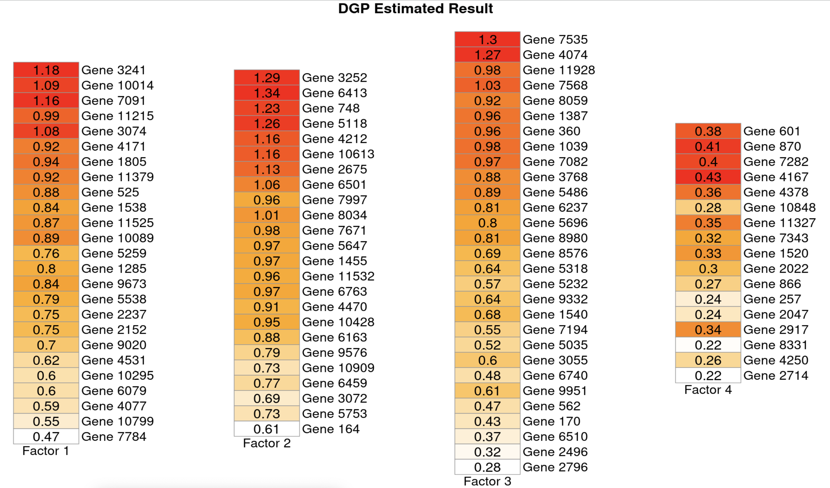
To evaluate the ability to estimate factor loadings, we consider two perspectives. First, for a specific factor, could the model identify all genes that were truly affected by this factor? Second, for a specific gene, could the model identify all factors that regulate this gene? To answer these questions, we calculated $95\%$ credible intervals for $l_{ga}$s and presented those $l_{ga}$s of which the interval did not contain $0$ in the heatmap, using posterior median estimates.

When the number of latent factors $k$ is correctly specified, our model returns satisfactory cross-correlation estimates under all data generation mechanisms considered (Figure 1). Furthermore, despite the initial (from the two-step approach) being poor, MCEM is able to propose estimates of the cross-correlations that rapidly approximate the truth (Supplementary Figure 2 shows an example under the scenario CS).

For the inference of $x_{ijg}^{\text{new}}$, $y_{ija}$, $l_{ga}$ using Gibbs-after-MCEM, Supplementary Table 1 lists the largest Rhat for each variable type, and reflect no apparent concerns over non-convergence. In terms of predicting gene expression, similar $\text{PWI}_{\mathbf{X}}$ is observed for both models. However, the DGP specification always leads to smaller $\text{MAE}_{\mathbf{X}}$ and narrower $\text{MWI}_{\mathbf{X}}$, even when the factors are uncorrelated in truth. This indicates more accuracy and less uncertainty in prediction (Table 1).

Summary results in Supplementary Table 2 suggest that estimating factors is generally easier when the true variability of factors is larger. A closer inspection of factor trajectories delineated in Supplementary Figure 3 further confirms this: under scenarios CL and UL, both DGP and IGP models are able to recover the shape of factor trajectories very well. This could be explained by the relatively strong expression of latent factors. In contrast, in the case of CS and US, where expression is relatively weak, recovery of details of factor shapes is harder: if factors are not correlated at all (scenario US), both DGP and IGP fail to recover the details at the $2$nd and $5$th time point, though the overall shape is still close to the truth. However, if factors are truly correlated (scenario CS), DGP is able to recover trajectories very well, due to its ability to borrow information from other related factors.

With regard to factor loading estimation, Figure 2 shows results under the scenario CS, and Supplementary Figures 4,5 and 6 show results for the remaining scenarios. Both DGP and IGP perform well at identifying the correct genes for a given factor under all scenarios. Both models also perform well at identifying the correct factors for a given gene under scenarios CL, UL and US, but under the scenario CS we observe that DGP still performs well whereas IGP performs less well. As can be seen from Figure 2, IGP specification leads to the result that genes estimated to be significantly loaded on the first and second factor also significantly load on the fourth factor. One possible explanation for this is that, if in truth, factors have strong signals and/or are not correlated at all (as in scenarios CL, UL and US), then it is relatively easy to distinguish contributions from different factors. In contrast, under the scenario CS where factors actually have weak signals and are highly-correlated (true correlation between factor 1 and 4 is $-0.69$, and correlation between factor 2 and 4 is $-0.71$, as can be found from Figure 1), it is more difficult. DGP specification explicitly takes the correlation among factors into consideration, allowing improved estimation.

We fitted the model with $k=2,3,\dots,10$ factors. We display results under $k=5$ after a comprehensive consideration of biological interpretation, computational cost and statistical prediction performance. Biologically, we found that $2$ biological pathways (immune response pathway and ribosome pathway; see Section 5.2 for details) were consistently identified when $k$ ranged from $3$ to $10$ while $k=2$ led to only $1$ pathway (immune response pathway) identified. Computationally, once $k$ was larger than $5$, our algorithm became slower as the parameter space was very large. Statistically, among the remaining models, $k=5$ showed the best prediction performance (see Supplementary Table 6).

In terms of the prediction performance, similar $\text{PWI}_{\mathbf{X}}$ is observed under BSFA-DGP ($0.951$) and BSFA-IGP ($0.956$); whereas $\text{MAE}_{\mathbf{X}}$ and $\text{MWI}_{\mathbf{X}}$ are both smaller under BSFA-DGP ($\text{MAE}_{\mathbf{X}}\ 0.211$; $\text{MWI}_{\mathbf{X}}\ 1.113$) than BSFA-IGP ($\text{MAE}_{\mathbf{X}}\ 0.217$; $\text{MWI}_{\mathbf{X}}\ 1.213$). This again demonstrates the advantage of reducing prediction error and uncertainty if cross-correlations among factors are taken into consideration.

Estimated factor trajectories using BSFA-DGP are displayed in Figure 3. Among all, factor $1$ is able to distinguish symptomatic people from asymptomatic people most clearly, and we find that its shape is largely similar to the “principal factor” identified in Chen et al., (2011). Despite the similarity, it is noteworthy that the trajectory of our factor $1$ is actually more individualized and informative than their principal factor (see Supplementary D.2 for discussion in detail). Compared with BSFA-IGP, our model BSFA-DGP reduces the variability within subject-specific trajectory, and consequently it slightly increases the difference between the symptomatic and asymptomatic. Although results look similar at first glance (Supplementary Figure 17), a more careful inspection reveals that BSFA-DGP has a shrinkage effect compared to BSFA-IGP. Take factor 1 as an example (similar observations for other factors). For the blue line at the bottom: at $38$ hours, it remains around $-1$ under BSFA-DGP while reaches as low as $-2$ under BSFA-IGP, making it harder to differentiate this symptomatic subject from asymptomatic subjects with red lines.

To identify the biological counterpart (i.e., pathway) of the statistical factor, we used the KEGG Pathway analysis of the online bioinformatics platform DAVID. We uploaded the total $11,961$ genes as the “Background” and the top $50$ genes loaded on each factor as the “Gene List”. This showed that factor 1 can be interpreted as ‘immune response pathway’ and factor 3 as ‘ribosome pathway’, while other factors have no known biological meaning (see Supplementary D.4). In addition, our MCEM algorithm estimates the magnitude of the cross-correlation coefficient to be $0.57$ between factors 1 and 3. This statistically moderate but biologically noteworthy correlation between these two pathways is consistent with existing biological knowledge (e.g. see Bianco and Mohr,, 2019, which concludes that ribosome biogenesis restricts innate immune responses to virus infection). This interrelated relationship would be missed by an approach that assumed independence between pathways, such as BSFA-IGP.

Throughout the following derivation, “$\circ$” denotes element-wise multiplication, “$-$” denotes observed data and all parameters in the model other than the parameter under derivation, “$||\mathbf{z}||^{2}$” denotes the sum of squares of each element of the vector $\mathbf{z}$, “$\text{diag}(\mathbf{z})$” denotes a diagonal matrix with the vector $\mathbf{z}$ as its main diagonal elements, “$\text{MVN}(\mathbf{z};\boldsymbol{\mu}_{\mathbf{z}},\Sigma_{\mathbf{z}})$” denotes that $\mathbf{z}$ follows a multivariate normal distribution with mean $\boldsymbol{\mu}_{\mathbf{z}},$ and variance $\Sigma_{\mathbf{z}}$, and similar interpretations apply to other distributions. “$\mathbf{z}^{T}$” denotes the transpose of the vector or matrix $\mathbf{z}$, and “pos” is short for ‘posterior probability’.

• •

  Full conditional for the latent factors $\operatorname{vec}({\mathbf{Y}_{i}}^{T}),i=1,\ldots,n$

  $\displaystyle\begin{split}f(\operatorname{vec}({\mathbf{Y}_{i}}^{T})|-)&=f(\operatorname{vec}({\mathbf{Y}_{i,\text{obs}}^{T}})|-)\cdot f(\operatorname{vec}({\mathbf{Y}_{i,\text{miss}}^{T}})|\operatorname{vec}({\mathbf{Y}_{i,\text{obs}}^{T}}),\Sigma_{\mathbf{Y}})\\ \end{split}$

  We first sample for $\operatorname{vec}({\mathbf{Y}_{i,\text{obs}}^{T}})$:

  $\displaystyle\begin{split}f(\operatorname{vec}({\mathbf{Y}_{i,\text{obs}}^{T}})|-)&\propto\text{MVN}(\operatorname{vec}({\mathbf{X}_{i}^{T}});\ \operatorname{vec}({\mathbf{M}_{i}^{T}})+\mathbf{L}_{i}^{*}\operatorname{vec}({\mathbf{Y}_{i,\text{obs}}^{T}}),\ \Sigma_{\mathbf{X}_{i}})\cdot\text{MVN}(\operatorname{vec}({\mathbf{Y}_{i,\text{obs}}^{T}});\ \mathbf{0},\ \Sigma_{\mathbf{Y}_{i,\text{obs}}})\\ &=\text{MVN}(\mu_{\mathbf{Y}_{i,\text{obs}}}^{\text{pos}},\ \Sigma_{\mathbf{Y}_{i,\text{obs}}}^{\text{pos}}),\end{split}$

  with

  $\displaystyle\begin{split}\Sigma^{pos}_{\mathbf{Y}_{i,\text{obs}}}&=[{\mathbf{L}_{i}^{*}}^{T}\Sigma_{\mathbf{X}_{i}}^{-1}\mathbf{L}_{i}^{*}+\Sigma_{\mathbf{Y}_{i,\text{obs}}}^{-1}]^{-1}\\ \mu^{\text{pos}}_{\mathbf{Y}_{i,\text{obs}}}&=\Sigma^{\text{pos}}_{\mathbf{Y}_{i,\text{obs}}}({\mathbf{L}_{i}^{*}}^{T}\Sigma_{\mathbf{X}_{i}}^{-1}(\operatorname{vec}({\mathbf{X}_{i}^{T}})-\operatorname{vec}({\mathbf{M}_{i}^{T}}))).\end{split}$

  Then we sample for $\operatorname{vec}({\mathbf{Y}_{i,\text{miss}}^{T}})$ from $f(\operatorname{vec}({\mathbf{Y}_{i,\text{miss}}^{T}})|\operatorname{vec}({\mathbf{Y}_{i,\text{obs}}^{T}}),\ \Sigma_{\mathbf{Y}})$, a MVN distribution due to the property of the DGP model (Shi and Choi,, 2011).
  

  In the above equations:

  • –

    $\Sigma_{\mathbf{Y}}$ is the covariance matrix of factor scores at full time $\mathbf{t}$, and $\Sigma_{\mathbf{Y}_{i,\text{obs}}}$ is a sub-matrix of it (at subject-specific time points);

  • –

    $\mathbf{L}_{i}^{*}$ is constructed using components of the factor loading matrix $\mathbf{L}$: $\mathbf{L}_{i}^{*}=(\mathbf{L}_{1}^{*},...,\mathbf{L}_{p}^{*})^{T}\in\mathbb{R}^{pq_{i}\times kq_{i}}$, where $(\mathbf{L}_{g}^{*})^{T}=({\text{diag}(l_{g1})}_{q_{i}\times q_{i}},...,{\text{diag}(l_{gk})}_{q_{i}\times q_{i}})\in\mathbb{R}^{q_{i}\times kq_{i}}$;

  • –

    $\Sigma_{\mathbf{X}_{i}}=\text{diag}(({\phi_{1}^{2}})_{\times q_{i}},...,({\phi_{p}^{2}})_{\times q_{i}})\in\mathbb{R}^{pq_{i}\times pq_{i}}$, where $\ ({\phi_{a}^{2}})_{\times q_{i}}$ represents a $q_{i}$-dimensional row vector consisting of the scalar ${\phi_{a}^{2}}$.

  Note that when coding the algorithm, there is no need to directly create the $pq_{i}\times pq_{i}$ diagonal matrix $\Sigma_{\mathbf{X}_{i}}^{-1}$ as the memory will be exhausted. To calculate the term ${\mathbf{L}_{i}^{*}}^{T}\Sigma_{\mathbf{X}_{i}}^{-1}$, we can use the property of multiplication of a diagonal matrix: post-multiplying a diagonal matrix is equivalent to multiplying each column of the first matrix by corresponding elements in the diagonal matrix.
  

• •

  Full conditional for the binary matrix $\mathbf{Z}$
  Let $\mathbf{Z}_{g\cdot}=(Z_{g1},...,Z_{gk})$ denote the $g$th row of the matrix $\mathbf{Z},\ g=1,...,p$; then,

  $\displaystyle\begin{split}f(\mathbf{Z}_{g\cdot}|-)&\propto\prod_{i=1}^{n}\text{MVN}(\mathbf{x}_{ig};\ \boldsymbol{\mu}_{ig}+(\mathbf{A}_{g\cdot}\circ\mathbf{Z}_{g\cdot})\mathbf{Y}_{i},\ \text{diag}(\phi_{g}^{2},\ q_{i}))\cdot\prod_{a=1}^{k}\text{Bernoulli}(Z_{ga};\pi_{a}),\end{split}$

  We calculate the posterior probability under $2^{k}$ possible values of $\mathbf{Z}_{g\cdot}$ based on the above formula, then sample with corresponding probability.

• •

  Full conditional for the regression coefficient matrix $\mathbf{A}$
  Let $\mathbf{A}_{g\cdot}=(A_{g1},...,A_{gk})$ denote the $g$th row of the matrix $\mathbf{A},\ g=1,...,p$; then,

  $\displaystyle\begin{split}f(\mathbf{A}_{g\cdot}|-)&\propto\prod_{i=1}^{n}\text{MVN}(\mathbf{x}_{ig};\ \boldsymbol{\mu}_{ig}+(\mathbf{A}_{g\cdot}\circ\mathbf{Z}_{g\cdot})\mathbf{Y}_{i},\ \text{diag}(\phi_{g}^{2},\ q_{i}))\cdot\text{MVN}(\mathbf{A}_{g\cdot};\ \mathbf{0},\ \text{diag}(\boldsymbol{\rho}^{2}))\\ &=\text{MVN}(\mathbf{A}_{g\cdot};\ \mu_{\mathbf{A}_{g\cdot}}^{\text{pos}},\ \Sigma_{\mathbf{A}_{g\cdot}}^{\text{pos}}),\end{split}$

  where

  $\displaystyle\begin{split}\Sigma_{\mathbf{A}_{g\cdot}}^{\text{pos}}&=({\frac{\text{diag}(\mathbf{Z}_{g\cdot})(\sum_{i=1}^{n}{\mathbf{Y}_{i}}^{T}\mathbf{Y}_{i})\text{diag}(\mathbf{Z}_{g\cdot})}{\phi^{2}_{g}}+\text{diag}(\frac{1}{\boldsymbol{\rho^{2}}}))}^{-1}\\ \mu_{\mathbf{A}_{g\cdot}}^{\text{pos}}&=\frac{\Sigma_{\mathbf{A}_{g\cdot}}(\text{diag}(\mathbf{Z}_{g\cdot})\sum_{i=1}^{n}{\mathbf{Y}_{i}}(\mathbf{x}_{ig}-\boldsymbol{\mu}_{ig}))}{\phi^{2}_{g}}.\end{split}$

  and $\boldsymbol{\rho^{2}}=(\rho^{2}_{1},...,\rho^{2}_{a})$.

• •

  Full conditional for the intercept $\mu_{ig},i=1,...,n;g=1,...,p$

  $\displaystyle\begin{split}f(\mu_{ig}|-)&\propto\prod_{j=1}^{q_{i}}\text{N}(x_{ijg};\mu_{ig}+\sum_{a=1}^{k}l_{ga}y_{ija},\phi^{2}_{g})\cdot\text{N}(\mu_{ig};\mu_{g},\sigma^{2}_{g})\\ &=\text{N}(\mu_{ig};\mu_{ig}^{\text{pos}},\ \sigma_{ig}^{2,\text{pos}}),\end{split}$

  where

  $\displaystyle\begin{split}\sigma_{ig}^{2,\text{pos}}&={(\frac{1}{\sigma^{2}_{g}}+\frac{q_{i}}{\phi^{2}_{g}})}^{-1}\\ \mu_{ig}^{\text{pos}}&=(\frac{\mu_{g}}{\sigma^{2}_{g}}+\frac{\sum_{j=1}^{q_{i}}(x_{ijg}-\sum_{a=1}^{k}l_{ga}y_{ija})}{\phi^{2}_{g}})\cdot\sigma_{ig}^{2,\text{pos}}\end{split}$

• •

  Full conditional for $\pi_{a},\ a=1,...,k$

  $\displaystyle\begin{split}f(\pi_{a}|-)&\propto\prod_{a=1}^{k}\text{Bernoulli}(Z_{ga};\pi_{a})\cdot\text{Beta}(\pi_{a};c_{0},d_{0})\\ &=\text{Beta}(c_{0}+\sum_{g=1}^{p}Z_{ga},\ d_{0}+\sum_{g=1}^{p}(1-Z_{ga}))\\ \end{split}$

• •

  Full conditional for $\rho_{a}^{2},\ a=1,...,k$

  $\displaystyle\begin{split}f(\rho_{a}^{2}|-)&\propto\prod_{g=1}^{p}\text{N}(A_{ga};0,\rho^{2}_{a})\cdot\text{Inverse-Gamma}(\rho_{a}^{2};c_{1},d_{1})\\ &=\text{Inverse-Gamma}(c_{1}+\frac{p}{2},\ d_{1}+\frac{1}{2}\sum_{g=1}^{p}A_{ga}^{2})\\ \end{split}$

• •

  Full conditional for $\sigma_{g}^{2},\ g=1,...,p$

  $\displaystyle\begin{split}f(\sigma_{g}^{2}|-)&\propto\prod_{i=1}^{n}\text{N}(\mu_{ig};\mu_{g},\sigma^{2}_{g})\cdot\text{Inverse-Gamma}(\sigma^{2}_{g};c_{2},d_{2})\\ &=\text{Inverse-Gamma}(c_{2}+\frac{1}{2}n,\ d_{2}+\frac{1}{2}\sum_{i=1}^{n}{(\mu_{ig}-\mu_{g}})^{2})\end{split}$

• •

  Full conditional for $\phi_{g}^{2},\ g=1,...,p$

  $\displaystyle\begin{split}f(\phi_{g}^{2}|-)&\propto\prod_{i=1}^{n}\text{MVN}(\mathbf{x}_{ig};\ \boldsymbol{\mu}_{ig}+(\mathbf{A}_{g\cdot}\circ\mathbf{Z}_{g\cdot})\mathbf{Y}_{i},\ \text{diag}(\phi_{g}^{2},\ q_{i}))\cdot\text{Inverse-Gamma}(\phi^{2}_{g};c_{3},d_{3})\\ &=\text{Inverse-Gamma}(c_{3}+\frac{1}{2}\sum_{i=1}^{n}q_{i},\ d_{3}+\frac{1}{2}\sum_{i=1}^{n}{||\mathbf{x}_{ig}-\boldsymbol{\mu}_{ig}-(\mathbf{A}_{g\cdot}\circ\mathbf{Z}_{g\cdot})\mathbf{Y}_{i}||}^{2})\end{split}$

• •

  Full conditional for predictions of gene expression (only implemented when assessing models’ prediction performance on the test dataset)

  Suppose that $\mathbf{X}_{i}^{\text{new}},\mathbf{Y}_{i}^{\text{new}}$ represent predicted gene expression and factor expression of the $i$th individual at new time points, respectively. The posterior predictive distribution under MCEM-algorithm-returned $\widehat{\boldsymbol{\Theta}}^{\text{MLE}}$ can be expressed as

  $\displaystyle\begin{split}f(\mathbf{X}_{i}^{\text{new}}|\ \widehat{\boldsymbol{\Theta}}^{\text{MLE}},\boldsymbol{\Omega})&=\int f(\mathbf{X}_{i}^{\text{new}},\mathbf{Y}_{i}^{\text{new}}|\ \widehat{\boldsymbol{\Theta}}^{\text{MLE}},\boldsymbol{\Omega})d\mathbf{Y}_{i}^{\text{new}}\\ &=\int f(\mathbf{X}_{i}^{\text{new}}|\mathbf{Y}_{i}^{\text{new}},\boldsymbol{\Omega})\cdot f(\mathbf{Y}_{i}^{\text{new}}|\widehat{\boldsymbol{\Theta}}^{\text{MLE}},\mathbf{Y}_{i,\text{obs}})d\mathbf{Y}_{i}^{\text{new}},\end{split}$

  where the first term of the integrand is a MVN because of the assumed factor model, and the second term is also a MVN because of the assumed DGP model on latent factor trajectories (Shi and Choi,, 2011). Therefore, once a sample of parameters $\boldsymbol{\Omega}^{r}$ is generated, the $r$th sample of ${\mathbf{Y}_{i}^{\text{new}}}$ can be generated from $f(\mathbf{Y}_{i}^{\text{new}}|\ \widehat{\boldsymbol{\Theta}}^{\text{MLE}},\mathbf{Y}_{i,\text{obs}}^{r})$, then the $r$th sample of ${\mathbf{X}_{i}^{\text{new}}}$ can be sampled from $f(\mathbf{X}_{i}^{\text{new}}|\ {\mathbf{Y}_{i}^{\text{new}}},\boldsymbol{\Omega}^{r})$.

References

- Álvarez et al., (2010) Álvarez, M., Luengo, D., Titsias, M., and Lawrence, N. D. (2010). Efficient multioutput gaussian processes through variational inducing kernels. In Proceedings of the Thirteenth International Conference on Artificial Intelligence and Statistics, pages 25–32. JMLR Workshop and Conference Proceedings.
- Alvarez and Lawrence, (2011) Alvarez, M. A. and Lawrence, N. D. (2011). Computationally efficient convolved multiple output Gaussian processes. The Journal of Machine Learning Research, 12:1459–1500.
- Bekker and ten Berge, (1997) Bekker, P. A. and ten Berge, J. M. (1997). Generic global indentification in factor analysis. Linear Algebra and its Applications, 264:255–263.
- Bhattacharya and Dunson, (2011) Bhattacharya, A. and Dunson, D. B. (2011). Sparse Bayesian infinite factor models. Biometrika, 98(2):291–306.
- Bianco and Mohr, (2019) Bianco, C. and Mohr, I. (2019). Ribosome biogenesis restricts innate immune responses to virus infection and dna. Elife, 8:e49551.
- Bonilla et al., (2007) Bonilla, E. V., Chai, K., and Williams, C. (2007). Multi-task Gaussian process prediction. Advances in Neural Information Processing Systems, 20.
- Booth and Hobert, (1999) Booth, J. G. and Hobert, J. P. (1999). Maximizing generalized linear mixed model likelihoods with an automated Monte Carlo EM algorithm. Journal of the Royal Statistical Society: Series B (Statistical Methodology), 61(1):265–285.
- (8) Boyle, P. and Frean, M. (2005a). Dependent Gaussian processes. Advances in Neural Information Processing Systems, 17:217–224.
- (9) Boyle, P. and Frean, M. (2005b). Multiple output Gaussian process regression.
- Caffo et al., (2005) Caffo, B. S., Jank, W., and Jones, G. L. (2005). Ascent-based Monte Carlo expectation–maximization. Journal of the Royal Statistical Society: Series B (Statistical Methodology), 67(2):235–251.
- Carvalho et al., (2008) Carvalho, C. M., Chang, J., Lucas, J. E., Nevins, J. R., Wang, Q., and West, M. (2008). High-dimensional sparse factor modeling: applications in gene expression genomics. Journal of the American Statistical Association, 103(484):1438–1456.
- Casella, (2001) Casella, G. (2001). Empirical Bayes Gibbs sampling. Biostatistics, 2(4):485–500.
- Chen et al., (2011) Chen, M., Zaas, A., Woods, C., Ginsburg, G. S., Lucas, J., Dunson, D., et al. (2011). Predicting viral infection from high-dimensional biomarker trajectories. Journal of the American Statistical Association, 106(496):1259–1279.
- Cheng et al., (2020) Cheng, L.-F., Dumitrascu, B., Darnell, G., Chivers, C., Draugelis, M., Li, K., et al. (2020). Sparse multi-output gaussian processes for online medical time series prediction. BMC medical informatics and decision making, 20(1):1–23.
- Conti et al., (2014) Conti, G., Frühwirth-Schnatter, S., Heckman, J. J., and Piatek, R. (2014). Bayesian exploratory factor analysis. Journal of econometrics, 183(1):31–57.
- Costello and Osborne, (2019) Costello, A. B. and Osborne, J. (2019). Best practices in exploratory factor analysis: Four recommendations for getting the most from your analysis. Practical assessment, research, and evaluation, 10(1):7.
- Dempster et al., (1977) Dempster, A. P., Laird, N. M., and Rubin, D. B. (1977). Maximum likelihood from incomplete data via the EM algorithm. Journal of the Royal Statistical Society: Series B (Methodological), 39(1):1–22.
- Dey et al., (2020) Dey, D., Datta, A., and Banerjee, S. (2020). Graphical Gaussian process models for highly multivariate spatial data. arXiv preprint arXiv:2009.04837.
- Gelman and Rubin, (1992) Gelman, A. and Rubin, D. B. (1992). Inference from iterative simulation using multiple sequences. Statistical Science, 7(4):457–472.
- Guan and Haran, (2019) Guan, Y. and Haran, M. (2019). Fast expectation-maximization algorithms for spatial generalized linear mixed models. arXiv preprint arXiv:1909.05440.
- Hensman et al., (2013) Hensman, J., Fusi, N., and Lawrence, N. D. (2013). Gaussian processes for big data. arXiv preprint arXiv:1309.6835.
- Hsu and Yang, (2012) Hsu, C.-L. and Yang, U.-C. (2012). Discovering pathway cross-talks based on functional relations between pathways. BMC Genomics, 13(7):1–15.
- Jones, (2004) Jones, G. L. (2004). On the Markov chain central limit theorem. Probability Surveys, 1:299–320.
- Kim et al., (2021) Kim, S. Y., Choe, E. K., Shivakumar, M., Kim, D., and Sohn, K.-A. (2021). Multi-layered network-based pathway activity inference using directed random walks: application to predicting clinical outcomes in urologic cancer. Bioinformatics, 37(16):2405–2413.
- Knowles and Ghahramani, (2011) Knowles, D. and Ghahramani, Z. (2011). Nonparametric Bayesian sparse factor models with application to gene expression modeling. The Annals of Applied Statistics, 5(2B):1534 – 1552.
- Konzen et al., (2021) Konzen, E., Cheng, Y., and Shi, J. Q. (2021). Gaussian process for functional data analysis: The GPFDA package for R. arXiv preprint arXiv:2102.00249.
- Ledermann, (1937) Ledermann, W. (1937). On the rank of the reduced correlational matrix in multiple-factor analysis. Psychometrika, 2(2):85–93.
- Levine and Casella, (2001) Levine, R. A. and Casella, G. (2001). Implementations of the Monte Carlo EM algorithm. Journal of Computational and Graphical Statistics, 10(3):422–439.
- Levine and Fan, (2004) Levine, R. A. and Fan, J. (2004). An automated (Markov chain) Monte Carlo EM algorithm. Journal of Statistical Computation and Simulation, 74(5):349–360.
- Li et al., (2020) Li, Y., Wen, Z., Hau, K.-T., Yuan, K.-H., and Peng, Y. (2020). Effects of cross-loadings on determining the number of factors to retain. Structural Equation Modeling: A Multidisciplinary Journal, 27(6):841–863.
- Liu et al., (2018) Liu, H., Cai, J., and Ong, Y.-S. (2018). Remarks on multi-output Gaussian process regression. Knowledge-Based Systems, 144:102–121.
- Lunn et al., (2013) Lunn, D., Jackson, C., Best, N., Thomas, A., and Spiegelhalter, D. (2013). The BUGS book. A Practical Introduction to Bayesian Analysis, Chapman Hall, London.
- Neath, (2013) Neath, R. C. (2013). On convergence properties of the Monte Carlo EM algorithm. In Advances in modern statistical theory and applications: a Festschrift in Honor of Morris L. Eaton, pages 43–62. Institute of Mathematical Statistics.
- Papastamoulis and Ntzoufras, (2022) Papastamoulis, P. and Ntzoufras, I. (2022). On the identifiability of Bayesian factor analytic models. Statistics and Computing, 32(2):1–29.
- Penny and Roberts, (2002) Penny, W. and Roberts, S. (2002). Bayesian multivariate autoregressive models with structured priors. IEE Proceedings-Vision, Image and Signal Processing, 149(1):33–41.
- Ramsay and Hooker, (2019) Ramsay, J. and Hooker, G. (2019). Dynamic data analysis: modeling data with differential equations. Springer.
- Ramsay et al., (2009) Ramsay, J., Hooker, G., and Graves, S. (2009). Introduction to functional data analysis. In Functional data analysis with R and MATLAB, pages 1–19. Springer.
- Richardson et al., (2016) Richardson, S., Tseng, G. C., and Sun, W. (2016). Statistical methods in integrative genomics. Annual review of statistics and its application, 3:181.
- Shi and Choi, (2011) Shi, J. Q. and Choi, T. (2011). Gaussian process regression analysis for functional data. CRC Press.
- Sofro et al., (2017) Sofro, A., Shi, J. Q., and Cao, C. (2017). Regression analysis for multivariate dependent count data using convolved Gaussian processes. arXiv preprint arXiv:1710.01523.
- Temate-Tiagueu et al., (2016) Temate-Tiagueu, Y., Seesi, S. A., Mathew, M., Mandric, I., Rodriguez, A., Bean, K., et al. (2016). Inferring metabolic pathway activity levels from RNA-Seq data. BMC Genomics, 17(5):493–503.
- Wei and Tanner, (1990) Wei, G. C. and Tanner, M. A. (1990). A Monte Carlo implementation of the EM algorithm and the poor man’s data augmentation algorithms. Journal of the American Statistical Association, 85(411):699–704.
- Wu, (1983) Wu, C. J. (1983). On the convergence properties of the EM algorithm. The Annals of Statistics, pages 95–103.
- Ximénez et al., (2022) Ximénez, C., Revuelta, J., and Castañeda, R. (2022). What are the consequences of ignoring cross-loadings in bifactor models? a simulation study assessing parameter recovery and sensitivity of goodness-of-fit indices. Frontiers in Psychology, 13:923877.
- Zaas et al., (2009) Zaas, A. K., Chen, M., Varkey, J., Veldman, T., Hero III, A. O., Lucas, J., et al. (2009). Gene expression signatures diagnose influenza and other symptomatic respiratory viral infections in humans. Cell Host & Microbe, 6(3):207–217.
- Zhao et al., (2016) Zhao, S., Gao, C., Mukherjee, S., and Engelhardt, B. E. (2016). Bayesian group factor analysis with structured sparsity. Journal of Machine Learning Research, 17(196):1–47.
-
•
Center to obtain (as defined in Section 4.2), which is input to BFRM for .
Input to GPFDA for , and construct using and .
Initialize the starting sample size ; the counter , which counts the total number of sample size increase, and specify its upper limit as , as described in Supplementary A.5.
2.1
Draw samples of from the Gibbs sampler in Section 3.2, where is constructed by and .
2.2
Retain samples by discarding burn-in and thinning.
2.3
Align post-processed samples using R package “factor.switch”.
2.4
Input aligned samples to GPFDA to obtain .
2.5
Calculate the lower bound proposed by Caffo et al., (2005) using , and (see Supplementary A.4.2 for details).