Dynamic Coherence-Based EM Ray Tracing Simulations in Vehicular Environments
Abstract
5G applications have become increasingly popular in recent years as the spread of fifth-generation (5G) network deployment has grown. For vehicular networks, mmWave band signals have been well studied and used for communication and sensing. In this work, we propose a new dynamic ray tracing algorithm that exploits spatial and temporal coherence.We evaluate the performance by comparing the results on typical vehicular communication scenarios with , which uses a combination of deterministic and stochastic models, and , which utilizes the deterministic model for simulations with given environment information. We also compare the performance of our algorithm on complex, urban models and observe a reduction in computation time by 36% compared to and by 30% compared to WinProp, while maintaining similar prediction accuracy.
Index Terms:
Ray tracing, 5G, mmWave, Vehicular communication.I Introduction
With the rise of millimeter-wave (mmWave) in 5G, many related technologies such as ray tracing (RT) have been studied and updated from sub 6 GHz band to mmWave band. RT can be used in many applications such as field prediction for radio network planning, RT-assist channel estimation for optimal beamforming techniques for mobile backhauling, real-time RT for assisted beamforming, and RT assisted localization [1]. In addition, mmWave has been studied through measurement campaigns for vehicular communications and sensing and has shown promising potential at high frequencies [2][3]. According to [4], the RADar-based COMmunication (RADCOM) technique enables simultaneous communication and sensing, which may further contribute to other technologies. While RADCOM is generating more research interest, ray tracing has been well studied since the 1990s. However, dynamic ray tracing is a recently developed idea for performing deterministic ray-based prediction in dynamic environments, where the environment shifts or objects in the scenes such as vehicles move. Efficient techniques have been proposed for fast ray tracing in such dynamic environments in sound [5][6] and visual rendering [7][8]. Dynamic ray tracing is also gaining more attention with the dramatic increase of mobile devices/users and the advent of wireless systems of traffic control and safety enforcement in the 5G era [9], where the transmitter stays more or less static while the surroundings change. On the other hand, we can also choose to apply ray-based propagation models to vehicular propagation with moving terminals and scatterers, as described in [10].
In this paper, we present a novel algorithm, which utilizes temporal and spatial coherence, for dynamic ray tracing for EM simulation in large environments and compare its performance in a typical vehicular environment with results from [21] and [17]. Our algorithm uses bounding volume hierarchy (BVH), a tree structure on a set of geometric objects, where all geometric objects that form the leaf nodes of the tree, are wrapped in bounding volumes; it can support efficient operations on sets of geometric objects in ray tracing. We implemented BVH with efficient techniques to recompute or update these hierarchies during each frame [11] and frame-to-frame coherence along with combining path tracing and radiosity methods [12]. Section II discusses related works and briefly introduces selected ray tracing software. Section III presents our proposed Dynamic Coherence-based EM ray tracing simulator (DCEM) details and the simulated environment. Section IV compares and discusses the simulation results. Section V concludes the paper and argues that our novel dynamic ray tracing approach is comparable to both academic and industrial ray tracing simulators. It also mentions potential future dynamic and real time ray tracing research. The key contributions of this paper are:
-
•
We propose the first dynamic coherence-based ray tracing algorithm at EM bands for fast and reliable RT simulations.
-
•
We develop a new ray tracing software, DCEM, which can work at mmWave frequencies, and show that it speeds up computation time by at least 30% with comparable prediction accuracy to other simulators like and .
-
•
We evaluate the performance of our ray tracing algorithm and system in large vehicular communication environments and highlight the benefits.
II Related work and available ray tracing software
Analysis of potential mmWave solutions to 5G has been conducted worldwide, and many measurements for indoor and outdoor scenes are described in [13] [14] [15]. However, the models built based on site-specific data could suffer significantly when moving to another site [16]. Another approach to building reliable models is an analytical approach, which can achieve high prediction accuracy when the environment is precisely built and computed with refined simulation setups. In our DCEM ray tracing software development process, we evaluate our results with and since they are 1) widely used for different scenarios and 2) not very difficult to install, with relatively detailed documents for their theory bases/user manual.
There are other RT software solutions currently in both industry and academia. We provide a brief description of the selected ray tracing software below and summarize the frequency range and applicable scenario in Table I.
WinProp [17] is an RT software from Altair that can support standard RT, Intelligent Ray Tracing (IRT), and Dominant Path models (DPM) at frequencies up to 100 GHz. It is also capable of simulating the spatial variability of the objects in various propagation scenarios.
Wireless Insite [18], developed by Remcom, can provide
ray tracing coupled with empirical and deterministic models for frequencies up to 100 GHz. It is accelerated by dimension reduction algorithms as well as performing accelerated computations using a graphics processing unit (GPU) and multi-threaded central processing unit (CPU) hardware acceleration.
NYUSIM [19] is an open-source mmWave channel model simulator developed by NYU Wireless based on years of measurements conducted at various frequencies. It is a generic statistical model that runs fast but does not take in site-specific information.
CloudRT [20] is an academic ray tracing tool created by members of the State Key Laboratory of Rail Traffic Control and Safety at Beijing Jiaotong University. This method is aimed at designing a high-performance cloud-based RT simulation platform that supports frequencies up to 325 GHz, includes all kinds of propagation mechanisms and mobile scattering objects, and is accelerated with a space partitioning algorithm and multi-thread computing.
is another academic ray tracing tool developed in [21] to analyze vehicle-to-vehicle channels in large environments [22]. This tool can simulate city-wide networks with tens of
thousands of vehicles on commodity hardware, providing hybrid RT along with empirical models. However, this work is based on MATLAB and only evaluated by measurements at 5.9 GHz.
| Simulator | Frequency range | Environment |
| WinProp | up to 100 GHz | Outdoor/indoor |
| Wireless Insite | up to 100 GHz | Outdoor/indoor |
| NYUSIM | up to 100 GHz | Outdoor/indoor |
| CloudRT | up to 325 GHz | Outdoor |
| 5.9 GHz | Outdoor | |
| DCEM | up to 72 GHz | Outdoor/indoor |
III DCEM and Simulation Scenario
Before going into the details of RT algorithms, we first define the concept of a ray in EM simulations. A ray is a high frequency approximation of Maxwell’s equations for propagating electromagnetic (EM) waves based on the electric and magnetic fields expressions as follows:
| (1) | ||||
| (2) |
where and are magnitude vectors and is the optical path length or eikonal. When and considering a series of wavefronts, the power flow lines perpendicular to the wavefronts are the rays, and they do not intersect if there is no focus point. Thus, the ray trajectory will be a straight line in a homogenous medium. The detailed mathematical derivation steps can be found in [23]. In conclusion, the ray, which helps analyze the different propagation mechanisms, is a straight line in a homogenous medium that carries energy and obeys the laws of reflection, transmission, and diffraction. In DCEM, we considered four kinds of rays:
-
•
Direct rays: If a ray goes from the source to the field point directly, the line of sight (LoS) propagation mechanism will be applied, and the pathloss will be simulated by
(3) where denotes the carrier frequency in GHz, is the 3D T-R separation distance, represents the path loss exponent (PLE), and is the attenuation term induced by the atmosphere [15].
-
•
Reflected and transmitted rays: If a ray is reflected or transmitted one or more times before reaching the field point, the ray will be segmented into different parts by reflected or transmitted points and be applied with the directed path loss model for each segment. The study in [1] shows that at the mmWave band, the signal power will be negligible at a high order of reflections and transmissions. In our proposed RT system, the limit of the maximum number of reflections/transmissions is set to 10 to balance the running time and accuracy by simulations trials.
-
•
Diffracted rays: The diffracted rays are more complicated than the two types of rays mentioned above, since one incident ray at the geometry edge can lead to a cone of diffracted rays. The uniform theory of diffraction (UTD) [24] is applied to calculate the diffraction coefficients here, and the detailed steps are followed as described in [25]. The upper bound of diffraction time simulated is set to 3 in this tool by practice.
- •
In addition to ray simulation, we also performed phase calculation.
For the acceleration methods, DCEM utilized three main algorithms: backward ray tracing from the receiver in the visibility determination step, the use of BVH while minimizing its rebuilding cost between frames, and propagation path caching for better frame coherence [12]. The idea of frame-to-frame coherence arises from the fact that if the object or transmitter does not drastically change its position between two adjacent frames, then most ray paths found in the previous frame can be reused in the current frame and this formulation can significantly reduce the computation times in low-speed dynamic simulations. The notion of coherence in ray tracing has been used for visual and aural rendering [27][28], but is not widely known in the context of EM ray tracing.
-
•
Backward ray tracing: In the backward RT algorithm, rays are cast from the listener or the receiver, rather than from each source. We observe that the reflected/diffracted rays coming from geometric primitives in the vicinity of the receiver, contribute more to the total received power. In fact, when casting rays from the source, only a few may reach the receiver and may not be the most perceptually important paths, resulting in more rays needing to be cast to get necessary propagation paths. The backward RT method can compute all the important paths while shooting fewer rays. The backward RT strategy also benefits from the fact that the number of rays no longer scales linearly with the number of sources.
Our overall algorithm proceeds as follows: 1) cast a random sphere of sampled rays, 2) record reflections and keep a hash table of visited propagation paths for each depth of reflection (up to a user defined threshold, 10 in DCEM), 3) generate a series of image receiver positions when encountering a new triangle series, 4) check the source to see if there is a valid path to the receiver, 5) if any edge is marked as a diffraction edge, consider the sources that lie in the diffraction shadow region from the receiver’s perspective and use the UTD diffraction formulation to determine the point on the edge at which diffraction occurs, then perform path validation back to the receiver as with reflection paths, 6) for each valid propagation path, the system calculates the total distance along the path, the direction of the path from the receiver, and the total attenuation and phase distortion along the path. -
•
Efficient BVH updating: BVHs have been widely used to accelerate the performance of ray tracing algorithms [29], and we take one step further to efficiently recompute or update these hierarchies during each frame. We do this because rebuilding BVHs is expensive in practice, and we minimize the cost by measuring BVH quality degradation between successive frames. The advantages of our method are: 1) it will update/rebuild at a time when necessary without any scene specific settings, 2) when there is little to no degradation, the rebuild would not be initiated, and 3) it is possible to just rebuild subtrees in some cases. These advantages improve the system computation efficiency; detailed evaluations can be found in [11].
-
•
Propagation path caching: The visibility hash tables as persistent caches are used to accelerate the path finding process from frame to frame. Once the valid paths are found, they are kept and updated until removed, i.e., at the beginning of each frame simulation, all triangle sequences in the hash tables are checked to see if the previous paths are still valid since the positions of source and receiver do not change much between frames. This method has significantly lowered the number of visibility rays cast each frame, leading to a higher overall frame rate and lower latency for real time applications. More details are described in [30][31].
In terms of the input, DCEM can take the environment description files including an “.obj” file for a description of the geometric primitives in the scene and an “.mtl” file for the material information of the objects in the environment. The following table highlights the material properties used in DCEM in terms of generating results and comparing with other methods [17][32]. For the outdoor scenario, we do not perform any penetration computations. The transmitter height is set to 2 meters in both cases, the frequency is set to 30 GHz, and the transmit power is 5W for outdoor and 0.5W for indoor scenes. The antenna is assumed to be ideal and omnidirectional. We use the modeled small European town built by Turbosquid [33] to perform RT simulations.
| Material | Thickness(mm) | Reflection coefficient | Penetration loss(dB) |
|---|---|---|---|
| Wall (Outdoor) | / | 0.8 | / |
| Wall (Indoor) | 10 | 0.7 | 20 |
| Glass (Indoor) | 5 | 0.74 | 5 |

IV Results Comparison and Discussion
We highlight some comparison results in this section. The outputs the received signal powers (RSP) of Vehicle-to-everything (V2X) and WinProp can generate heatmaps of RSP. We compare the results with for outdoor vehicular communication scenarios and with WinProp for indoor scenes to evaluate the accuracy of our system DCEM, based on measurements data [17][21].
IV-A Outdoor Environment
We highlight the results and visualizations from in Fig. 2 . The RSP of is a combination of large-scale variations computed by deterministic models and small-scale variations estimated from stochastic models.

Fig. 3 hightlights a localized region in the urban environment in .

Fig. 4 shows a simulation comparison between DCEM and within a street in the 3D model urban environment. We define the units and positions of interest to perform simulations in and run the simulation three times to evaluate the small-scale scholastic variations and compare them with the ray tracing results from DCEM. We observe a good match in the predicted positions in RSP and time delay, and the mean of RSP shows an average difference of 1.7 dBm.

IV-B Indoor Environment
We compare the simulation results of the indoor environments (shown in Fig. 5) computed using WinProp and DCEM. The signal frequency is set to 30GHz and the TX height is set at 2 meters. The indoor environment consists of walls, doors, and windows with different reflection/transmission/diffraction coefficients.

The output one-shot heatmaps of the indoor environment produced by WinProp and DCEM are shown in Fig. 6 and Fig. 7. We see from the two heatmaps that DCEM predictions show behaviors similar to WinProp results. There is, however, some blurred prediction area towards the boundary of the environment, which might be resulting from different boundary condition settings.

A total of three testing cases were simulated with different Tx locations. The other two pairs of heatmap comparisons are shown below with different TX locations in the environment (see Fig. 7 and Fig. 8).


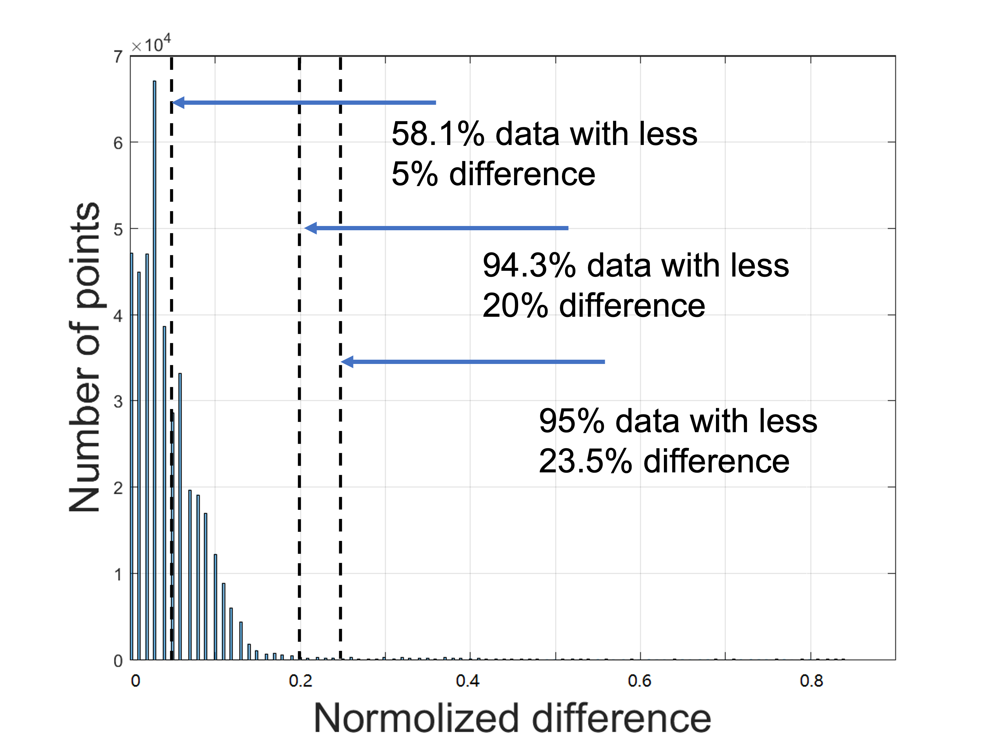
The histogram of the difference between the predicted heatmaps from WinProp and DCEM of Site 2 is shown below. According to the numbers, about 58.1% of the prediction difference is less than 5% and 95% of the prediction difference is less than 23.5%.
The histogram comparison of Site 1 and Site 3 is also attached below.

IV-C Runtime Comparison
We summarize the working time of the simulations in the following tables.
The parameter settings of the comparison between and DCEM are: runs with reflection and diffraction enabled and DCEM runs with 2000 shooting rays, max 2 reflections, 2 transmissions, and 1 diffraction. We run the tests three times to mitigate computer performance variation. We see from the three test case runs that DCEM has an average of 36.5% speedup compared to , which might results from the both fast ray tracing algorithm improvements and software differences ( in MATLAB and DCEM in C++).
| Simulator | Runtime test1 | Runtime test2 | Runtime test3 |
|---|---|---|---|
| 33.5s | 32.3s | 32.3s | |
| DCEM | 20.5s | 21.2s | 20.6s |
Table IV shows the comparison between Winrprop and DCEM with the whole simulation process, including parsing the modeled village file. WinProp takes a longer time. In terms of the overall preprocessing time, DCEM has improved efficiency in terms of running time by 30.4%, as compared to WinProp. When taking only the ray tracing simulation time into consideration or performing ray tracing in a simple indoor environment, we set the parameters as follows: WinProp resolution range is 0.02m and it takes max 2 reflections, 2 transmissions, and 1 diffraction by 3D ray tracing model, while DCEM runs with 2000 shooting rays, max 2 reflections, 2 transmissions, and 1 diffraction, Table IV shows that WinProp has a slightly better, but similar computation time to DCEM.
| Simulator | Runtime test1 | Runtime test2 |
|---|---|---|
| WinProp | 60min | 65min |
| DCEM | 45min | 42min |
| Simulator | Runtime case1 | Runtime case2 | Runtime case3 |
|---|---|---|---|
| WinProp | 26s | 25s | 29s |
| DCEM | 30s | 31s | 35s |
V Conclusion
In this paper, we proposed a reliable and fast RT simulator at EM bands for a typical vehicular communication scenario with a novel dynamic ray tracing algorithm that exploits spatial and temporal coherence. We performed simulations to compare our method with two other well-known RT simulators. The Ericsson’s 5G demo from a recent NVIDIA Omniverse keynote speech [34] showed a ray tracing simulation between base stations and vehicles in a complex environment. Therefore, our next step will be to improve the capabilities of the DCEM to perform RT simulations in more complex and dynamic environments in real time.
References
- [1] Fuschini, Franco, et al.“Ray tracing propagation modeling for future small-cell and indoor applications: A review of current techniques.” Radio Science 50.6 (2015): 469-485.
- [2] Ben-Dor, Eshar, et al.“Millimeter-wave 60 GHz outdoor and vehicle AOA propagation measurements using a broadband channel sounder.” 2011 IEEE Global Telecommunications Conference-GLOBECOM 2011. IEEE, 2011.
- [3] Samimi, Mathew K., and Theodore S. Rappaport.“3-D millimeter-wave statistical channel model for 5G wireless system design.” IEEE Transactions on Microwave Theory and Techniques 64.7 (2016): 2207-2225.
- [4] Lübke, Maximilian, et al. “Comparing mmWave Channel Simulators in Vehicular Environments.” 2021 IEEE 93rd Vehicular Technology Conference (VTC2021-Spring). IEEE, 2021.
- [5] Schissler, Carl, and Dinesh Manocha. “Interactive sound rendering on mobile devices using ray-parameterized reverberation filters.” arXiv preprint arXiv:1803.00430 (2018).
- [6] Manocha, Dinesh, and Ming C. Lin. “Interactive sound rendering.” 2009 11th IEEE International Conference on Computer-Aided Design and Computer Graphics. IEEE, 2009.
- [7] J. Burgess, “RTX on—The NVIDIA Turing GPU,” in IEEE Micro, vol. 40, no. 2, pp. 36-44, 1 March-April 2020, doi: 10.1109/MM.2020.2971677.
- [8] Steven G. Parker, James Bigler, Andreas Dietrich, Heiko Friedrich, Jared Hoberock, David Luebke, David McAllister, Morgan McGuire, Keith Morley, Austin Robison, and Martin Stich. 2010. OptiX: a general purpose ray tracing engine. ACM Trans. Graph. 29, 4, Article 66 (July 2010), 13 pages. DOI:https://doi.org/10.1145/1778765.1778803
- [9] Bilibashi, D., E. M. Vitucci, and V. Degli-Esposti. “Dynamic ray tracing: Introduction and concept.” 2020 14th European Conference on Antennas and Propagation (EuCAP). IEEE, 2020.
- [10] Azpilicueta, Leyre, Cesar Vargas-Rosales, and Francisco Falcone. “Intelligent vehicle communication: Deterministic propagation prediction in transportation systems.” IEEE Vehicular Technology Magazine 11.3 (2016): 29-37.
- [11] Lauterbach, Christian, et al. “RT-DEFORM: Interactive ray tracing of dynamic scenes using BVHs.” 2006 IEEE Symposium on Interactive Ray Tracing. IEEE, 2006.
- [12] Schissler, Carl, Ravish Mehra, and Dinesh Manocha. “High-order diffraction and diffuse reflections for interactive sound propagation in large environments.” ACM Transactions on Graphics (TOG) 33.4 (2014): 1-12.
- [13] Rappaport, Theodore S., et al. “Millimeter wave mobile communications for 5G cellular: It will work!.” IEEE access 1 (2013): 335-349.
- [14] Degli-Esposti, Vittorio, et al. “Measurement and modelling of scattering from buildings.” IEEE Transactions on Antennas and Propagation 55.1 (2007): 143-153.
- [15] MacCartney Jr, George R., et al. “Millimeter wave wireless communications: New results for rural connectivity.” Proceedings of the 5th workshop on all things cellular: operations, applications and challenges. 2016.
- [16] Nguyen, Huan Cong, et al. “Evaluation of empirical ray-tracing model for an urban outdoor scenario at 73 GHz E-band.” 2014 IEEE 80th Vehicular Technology Conference (VTC2014-Fall). IEEE, 2014.
- [17] “WinProp: Wireless connectivity”. Accessed on Apr 8, 2022. [Online]. https://www.altair.com/electromagnetics-applications/
- [18] “Wireless Insite 3D Wireless Prediction Software”. Accessed on Apr 8, 2022. [Online]. https://www.remcom.com/wireless-insite-em-propagation-software/
- [19] Sun, Shu. “NYUSIM user manual.” New York University and NYU WIRELESS (2017).
- [20] “CLoudRT: High Performance Antenna, Propagation and Channel modeling Platform”. Accessed on Apr 8, 2022. [Online]. http://cn.raytracer.cloud/
- [21] M. Boban, J. Barros, and O. K. Tonguz, “Geometry-based vehicle-tovehicle channel modeling for large-scale simulation,” IEEE Trans. Veh. Technol., vol. 63, no. 9, pp. 4146–4164, Nov. 2014.
- [22] “: geometry-based, efficient propagation model for vehicle-to-vehicle (V2V) and vehicle-to-infrastructure (V2I) communication”. Accessed on Apr 8, 2022. [Online]. http://vehicle2x.net/
- [23] Yun, Zhengqing, and Magdy F. Iskander. “Ray tracing for radio propagation modeling: Principles and applications.” IEEE Access 3 (2015): 1089-1100.
- [24] Kouyoumjian, Robert G., and Prabhakar H. Pathak. “A uniform geometrical theory of diffraction for an edge in a perfectly conducting surface.” Proceedings of the IEEE 62.11 (1974): 1448-1461.
- [25] Balanis, Constantine A. Advanced engineering electromagnetics. John Wiley & Sons, 2012.
- [26] Hossain, Ferdous, et al. “An efficient 3-D ray tracing method: prediction of indoor radio propagation at 28 GHz in 5G network.” Electronics 8.3 (2019): 286.
- [27] Okoro, Chukwuemeka, et al. ”Modeling, optimization, and validation of an extended-depth-of-field optical coherence tomography probe based on a mirror tunnel.” Applied Optics 60.8 (2021): 2393-2399.
- [28] Meister, Daniel, et al. ”A survey on bounding volume hierarchies for ray tracing.” Computer Graphics Forum. Vol. 40. No. 2. 2021.
- [29] Smits, Brian. “Efficiency issues for ray tracing.” Journal of Graphics Tools 3.2 (1998): 1-14.
- [30] Schissler, Carl, and Dinesh Manocha. “Gsound: Interactive sound propagation for games.” Audio Engineering Society Conference: 41st International Conference: Audio for Games. Audio Engineering Society, 2011.
- [31] Rungta, Atul, et al. “Diffraction kernels for interactive sound propagation in dynamic environments.” IEEE transactions on visualization and computer graphics 24.4 (2018): 1613-1622.
- [32] Zhao, Hang, et al. ”28 GHz millimeter wave cellular communication measurements for reflection and penetration loss in and around buildings in New York city.” 2013 IEEE international conference on communications (ICC). IEEE, 2013.
- [33] “Turbosquid: 3D Models for Professionals”. Accessed on Apr 8, 2022. [Online]. https://www.turbosquid.com/
- [34] “Ericsson Builds Digital Twins for 5G Networks in NVIDIA Omniverse”. Accessed on Apr 8, 2022. [Online]. https://blogs.nvidia.com/blog/2021/11/09/ericsson-digital-twins-omniverse/
VI Appendix
We also include LOS and NLOS comparisons between NYUSIM and DCEM here. The following figures show the environment setups and the simulation results from NYUSIM Fig. 12 - Fig. 13 and from DCEM Fig. 14 - Fig. 15.


These results showed that the proposed algorithm works well with moving object in urban environment. Our future work will be simulating more complex scenes with more moving objects and complex building blocks.