Dynamic Adaptation Gains for Nonlinear Systems with Unmatched Uncertainties

Brett T. Lopez¹ and Jean-Jacques Slotine² ¹Verifiable and Control-Theoretic Robotics Laboratory, University of California, Los Angeles, Los Angeles CA, [email protected]²Nonlinear Systems Laboratory, Massachusetts Institute of Technology, Cambridge MA, [email protected]

Abstract

We present a new direct adaptive control approach for nonlinear systems with unmatched and matched uncertainties. The method relies on adjusting the adaptation gains of individual unmatched parameters whose adaptation transients would otherwise destabilize the closed-loop system. The approach also guarantees the restoration of the adaptation gains to their nominal values and can readily incorporate direct adaptation laws for matched uncertainties. The proposed framework is general as it only requires stabilizability for all possible models.

Index Terms:

Adaptive control, uncertain systems.

I Introduction

Adaptive control of systems with unmatched uncertainties, i.e., model perturbations outside the span of the control input matrix, is notoriously difficult because the uncertainties cannot be directly canceled by the control input. This is especially true for nonlinear systems where combining a stable model estimator with a nominal feedback controller does not necessarily yield a stable closed-loop system without imposing limits on the growth rate of the uncertainties, so as to prevent finite escape. The prevailing approach for handling nonlinear systems with unmatched uncertainties has been to construct nominal feedback controllers that are robust to time-varying parameter estimates [1]. More precisely, one seeks to construct an input-to-state stable control Lyapunov function (ISS-clf) [2] which, by construction, ensures the system converges to a region near the desired state despite parameter estimation error and transients. Once an ISS-clf and corresponding controller are known, then any stable model estimator can be employed without concern of instability. From a theoretical standpoint, this framework guarantees stable closed-loop control and estimation despite unmatched uncertainties but requires constructing an ISS-clf – a nontrivial task unless the system takes a particular structure.

The approach discussed above is categorized as indirect adaptive control and entails combining a robust controller with a stable model estimator. Conversely, direct adaptive control uses Lyapunov-like stability arguments to construct a parameter adaptation law that guarantees the state converges to a desired value. This eliminates the robustness requirements inherent to indirect adaptive control which, in some ways, simplifies design. However, since unmatched uncertainties cannot be directly canceled through control, it is necessary to construct a family of Lyapunov functions that depend on the estimates of the unmatched parameters. This model dependency introduces sign-indefinite terms (related to the parameter estimation transients) in the stability proof that require sophisticated direct adaptive control schemes to achieve stable closed-loop control and adaptation. Adaptive control Lyapunov functions (aclf) where proposed to cancel the problematic transient terms by synthesizing a family of clf’s for a modified dynamical system that depends on the family of clf’s [3]. Recently, [4] proposed a method that adjusts the adaptation gain online to cancel the undesirable transient terms and requires no modifications to the standard clf definition or dynamical system of interest.

The main contribution of this work is a new direct adaptive control methodology which generalizes and improves the online adaptation gain adjustment approach from [4], subsequently called dynamic adaptation gains, yielding a superior framework for handling various forms of model uncertainties. The new framework has two distinguishing properties: 1) adaptation gains are individually adjusted online to prevent parameter adaptation transients from destabilizing the system and 2) the adaptation gain is guaranteed to return to its nominal value asymptotically. Conceptually, the adaptation gain is lowered, i.e., adaptation slowed, for parameters whose transients is destabilizing; the adaptation gain then returns to its nominal once the transients subsides. Noteworthy properties are examined, e.g., handling of matched uncertainties, and several forms of the dynamic adaptation gain update law are derived. The approach only relies on stabilizability of the uncertain system so it is a very general framework. Simulation results of a nonlinear system with unmatched and matched uncertainties demonstrates the approach.

Notation: The set of positive and strictly-positive scalars will be denoted as $\mathbb{R}_{\geq 0}$ and $\mathbb{R}_{>0}$ , respectively. The shorthand notation for a function $T$ parameterized by a vector $a$ with vector argument $s$ will be $T_{a}(s)=T(s;a)$ . The partial derivative of a function $N(x,y)$ will sometimes denoted as $\nabla_{x}N(x,y)=\frac{\partial N}{\partial x}$ where the subscript on $\nabla$ is omitted when there is no ambiguity.

II Problem Formulation

This work addresses control of uncertain dynamical systems of the form

\dot{x}=f(x,t)-\Delta(x,t)^{\top}\theta+B(x,t)u,

(1)

with state $x\in\mathbb{R}^{n}$ , control input $u\in\mathbb{R}^{m}$ , nominal dynamics $f:\mathbb{R}^{n}\times\mathbb{R}_{\geq 0}\rightarrow\mathbb{R}^{n}$ , and control input matrix $B:\mathbb{R}^{n}\times\mathbb{R}_{\geq 0}\rightarrow\mathbb{R}^{n\times m}$ . The uncertain dynamics are a linear combination of known regression vectors $\Delta:\mathbb{R}^{n}\times\mathbb{R}_{\geq 0}\rightarrow\mathbb{R}^{p\times n}$ and unknown parameters $\theta\in\mathbb{R}^{p}$ . We assume that Equation 1 is locally Lipschitz uniformly and that the state $x$ is measured. The following assumption is made on the unknown parameters $\theta$ .

Assumption 1.

The unknown parameters $\theta$ belong to a known compact convex set $\Theta\subset\mathbb{R}^{p}$ .

An immediate consequence of Assumption 1 is that the parameter estimation error $\ \tilde{\theta}\triangleq\hat{\theta}-\theta\$ must also belong to a known compact convex set $\tilde{\Theta}$ . Each parameter must then have a finite maximum error where $|\tilde{\theta}_{i}|\leq\tilde{\vartheta}_{i}<\infty$ for $i=1,\dots,p$ .

III Main Results

III-A Overview

This section presents the main results of this work. We first review the definition of the unmatched control Lyapunov function [4] and its role in the proposed approach. We then derive the first main result followed by several noteworthy extensions, e.g., the scenario where unmatched and matched uncertainties are present in addition to augmenting the adaptation law with model estimation (composite adaptation). We also present the the so-called leakage modification that guarantees the adaptation gains return to their nominal values asymptotically. Conceptually, the proposed approach relies on adjusting the adaptation gain of individual parameter estimates online to prevent destabilization induced by parameter adaptation transients. This is in stark contrast to [4] where a single gain for all parameters was adjusted. Consequently this work can be considered a more general and natural formulation of [4].

III-B Unmatched Control Lyapunov Functions

Similar to [4], the so-called unmatched control Lyapunov function will be used through this letter.

Definition 1 (cf. [4]).

A smooth, positive-definite function $V_{\theta}:\mathbb{R}^{n}\times\mathbb{R}^{p}\times\mathbb{R}_{\geq 0}\rightarrow\mathbb{R}_{\geq 0}$ is an unmatched control Lyapunov function (uclf) if it is radially unbounded in $x$ and for each $\theta\in\Theta\subset\mathbb{R}^{p}$

\displaystyle\underset{u\in\mathbb{R}^{m}}{\mathrm{inf}}\left\{\frac{\partial V_{\theta}}{\partial t}+\frac{\partial V_{\theta}}{\partial x}^{\top}\left[f-\Delta^{\top}\theta+Bu\right]\right\}\leq-Q_{\theta}

where $Q_{\theta}:\mathbb{R}^{n}\times\mathbb{R}^{p}\rightarrow\mathbb{R}_{\geq 0}$ is continuously differentiable, radially unbounded in $x$ , and positive-definite.

Remark 1.

Definition 1 can also be stated in terms of a contraction metric [5], see [4, Def. 1] for more details.

Definition 1 is noteworthy because the existence of an uclf is equivalent (see [4, Prop. 1]) to system Equation 1 being stabilizable for all $\theta\in\Theta$ . This is the weakest possible requirement one can impose on Equation 1 and therefore showcases the generality of the approach. Definition 1 involves constructing a clf for each possible model realization, i.e., a family of clf’s, so convergence to the desired equilibrium can be achieved if a suitable adaptation law can be derived. Pragmatically, this can be done analytically, e.g., via backstepping, or numerically via discretization or sum-of-squares programming with the uclf search occurring over the state-parameter space. Definition 1 adopts the certainty equivalence principle philosophy: design a clf (or equivalently a controller) as if the unknown parameters are known and simply replace them with their estimated values online. This intuitive design approach is not generally possible for nonlinear systems with unmatched uncertainties unless additional robustness properties are imposed or the system be modified – both representing a departure from certainty equivalence. The approach developed in this work completely bypasses any additional requirements or system modifications by instead adjusting the adaptation gain online where the so-called adaptation gain update law yields a stable closed-loop system. In other words, the proposed dynamic adaptation gains method expands the use of the certainty equivalence principle to general nonlinear systems with unmatched uncertainties, simplifying the design of stable adaptive controllers.

III-C Dynamic Adaptation Gains

The proposed method involves adjusting the adaptation gain—typically denoted as a scalar $\gamma$ or symmetric positive-definite matrix $\Gamma$ is the literature—to prevent the parameter adaptation transients from destabilization the closed-loop system. It is convenient to express the adaptation gain as a function of a scalar argument that has certain properties. We will make use of the following definition in deriving an adaptation gain update law that achieves closed-loop stability.

Definition 2.

An admissible dynamic adaptation gain $\gamma:\mathbb{R}\rightarrow\mathbb{R}_{>0}$ is a function with scalar argument $\rho$ such that $\gamma(0)=\bar{\gamma}$ is the nominal adaptation gain, $\lim_{\rho\rightarrow-\infty}\gamma(\rho)=c>0$ , and $0<\nabla\gamma(\rho)<\infty$ .

Remark 2.

There are several functions at the disposal of the designer when selecting an admissible dynamic adaptation gain. Two examples are $\gamma(\rho)=\bar{\gamma}\,(\frac{0.9}{\rho^{2}+1}+0.1)$ or $\gamma(\rho)=\bar{\gamma}\,(0.9\,\mathrm{exp}(\rho/\tau)+0.1)$ .

With Definitions 1 and 2, we are now ready to state the first main theorem of this work.

Theorem 1.

Consider the uncertain system Equation 1 with $x_{d}$ being the desired equilibrium point. If an uclf $\,V_{\theta}(x,t)\,$ exists, then $x\rightarrow x_{d}$ asymptotically with the adaptation law

\dot{\hat{\theta}}=-\,\mathrm{diag}(\gamma_{1}(\rho_{1}),\dots,\gamma_{p}(\rho_{p}))\,\Delta(x,t)\frac{\partial V_{\hat{\theta}}}{\partial x}

(2a)

where each $\gamma_{i}(\cdot)$ is an admissible dynamic adaptation gain whose update law satisfies

\dot{\gamma}_{i}(\rho_{i})\leq-2\frac{\gamma_{i}(\rho_{i})^{2}}{(\eta_{i}-\tilde{\theta}^{2}_{i})}\frac{\partial V_{\hat{\theta}}}{\partial\hat{\theta}_{i}}\,\dot{\hat{\theta}}_{i}

(2b)

for $\eta_{i}>\tilde{\vartheta}_{i}\geq\tilde{\theta}_{i}$ with $i=1,\dots,p$ .

Proof.

Consider the Lyapunov-like function

V_{c}(t)=V_{\hat{\theta}}(x,t)+\frac{1}{2}\sum_{i=1}^{p}\frac{(\tilde{\theta}_{i}^{2}-\eta_{i})}{\gamma_{i}(\rho_{i})},

(3)

where $\tilde{\theta}=\hat{\theta}-\theta$ and $\eta_{i}>\tilde{\vartheta}_{i}\geq\tilde{\theta}_{i}$ with $\eta_{i}$ finite. Differentiating Equation 3 yields

	$\displaystyle\dot{V}_{c}(t)=$	$\displaystyle\,{\frac{\partial V_{\hat{\theta}}}{\partial t}}+\frac{\partial V_{\hat{\theta}}}{\partial x}^{\top}[f(x,t)-\Delta(x,t)^{\top}\theta+{B(x,t)}u]$
		$\displaystyle+\sum_{i=1}^{p}\biggl{[}\frac{\partial V_{\hat{\theta}}}{\partial\hat{\theta}_{i}}\,\dot{\hat{\theta}}_{i}+\frac{\tilde{\theta}_{i}}{\gamma_{i}(\rho_{i})}\dot{\hat{\theta}}_{i}+\frac{1}{2}\frac{(\eta_{i}-\tilde{\theta}_{i}^{2})}{\gamma_{i}(\rho_{i})^{2}}\,\dot{\gamma}_{i}(\rho_{i})\biggr{]}.$

Since $V_{\hat{\theta}}(x,t)$ is an uclf then

	$\displaystyle\dot{V}_{c}(t)\leq$	$\displaystyle\,-Q_{\hat{\theta}}(x)+\frac{\partial V_{\hat{\theta}}}{\partial x}^{\top}\Delta(x,t)^{\top}\tilde{\theta}$
		$\displaystyle+\sum_{i=1}^{p}\biggl{[}\frac{\partial V_{\hat{\theta}}}{\partial\hat{\theta}_{i}}\,\dot{\hat{\theta}}_{i}+\frac{\tilde{\theta}_{i}}{\gamma_{i}(\rho_{i})}\dot{\hat{\theta}}_{i}+\frac{1}{2}\frac{(\eta_{i}-\tilde{\theta}_{i}^{2})}{\gamma_{i}(\rho_{i})^{2}}\,\dot{\gamma}_{i}(\rho_{i})\biggr{]}.$

Noting

\sum_{i=1}^{p}\frac{\tilde{\theta}_{i}}{\gamma_{i}(\rho_{i})}\dot{\hat{\theta}}_{i}=\tilde{\theta}^{\top}[\mathrm{diag}(\gamma_{1}(\rho_{1}),\dots,\gamma_{p}(\rho_{p}))]^{-1}\,\dot{\hat{\theta}}

then applying Equation 2a yields

\displaystyle\dot{V}_{c}(t)

\displaystyle\leq-Q_{\hat{\theta}}(x)+\sum_{i=1}^{p}\biggl{[}\frac{\partial V_{\hat{\theta}}}{\partial\hat{\theta}_{i}}\,\dot{\hat{\theta}}_{i}+\frac{1}{2}\frac{(\eta_{i}-\tilde{\theta}_{i}^{2})}{\gamma_{i}(\rho_{i})^{2}}\,\dot{\gamma}_{i}(\rho_{i})\biggr{]}.

If $\dot{\gamma}_{i}(\rho_{i})$ is chosen so Equation 2b is satisfied, then the term in brackets is negative so $\dot{V}_{c}(t)\leq-Q_{\hat{\theta}}(x)<0$ if $x\neq x_{d}$ . Hence, $V_{c}(t)$ is non-increasing so $V_{\hat{\theta}}(x,t)$ and $\tilde{\theta}$ are bounded since $\gamma_{i}(\rho_{i})$ is lower-bounded and $\eta_{i}$ is bounded by construction. Since $V_{\hat{\theta}}(x,t)$ is radially unbounded then $x$ must also be bounded. By definition, $Q_{\hat{\theta}}(x)$ is continuously differentiable so $\dot{Q}_{\hat{\theta}}(x)$ is bounded for bounded $x$ , $\tilde{\theta}$ and therefore $Q_{\hat{\theta}}(x)$ is uniformly continuous. Since $V_{c}(t)$ is nonincreasing and bounded from below then $\lim_{t\rightarrow\infty}\int_{0}^{t}Q_{\hat{\theta}}(x(\tau))\,d\tau~{}{\leq}~{}V_{c}(0)-\lim_{t\rightarrow\infty}V_{c}(t)$ exists and is finite so by Barbalat’s lemma $\lim_{t\rightarrow\infty}Q_{\hat{\theta}}(x(t))\rightarrow 0$ . Recalling $Q_{\hat{\theta}}(x)=0\iff x=x_{d}$ then we can conclude $x(t)\rightarrow x_{d}$ as $t\rightarrow\infty$ as desired. ∎

Remark 3.

Since the unknown parameters belong to a compact convex set $\Theta$ then one can employ the projection operator $\mathrm{Proj}_{\Theta}(\cdot)$ to ensure $\hat{\theta}\in\Theta$ without affecting stability [6, 7].

Remark 4.

Equation 2b is expressed as an update to $\dot{\gamma}_{i}(\rho_{i})$ to make the dynamic adaptation gain interpretation more obvious. For implementation, one should rewrite Equation 2b as a bound on $\dot{\rho}_{i}$ via the chain rule. Note $\nabla\gamma_{i}(\rho_{i})$ in invertible by Definition 2.

Before deriving various implementable forms of the dynamic adaptation gain update law, it is instructive to analyze its general behavior. For the case where a parameter’s adaptation transients is destabilizing, i.e., $\tfrac{\partial V_{\hat{\theta}}}{\partial\hat{\theta}_{i}}\tfrac{d}{dt}\hat{\theta}_{i}>0$ for some $i$ , we see from Equation 2b that $\dot{\gamma}_{i}(\rho_{i})<0$ so the adaptation gain decreases to prevent destabilization. In other words, the adaptation rate is slowed for parameters whose adaptation transients could cause instability. Note that there is no concern of the adaptation gain $\gamma_{i}(\rho_{i})$ becoming negative since $\gamma_{i}(\rho_{i})$ must be an admissible dynamic adaptation gain so, by definition, $\gamma_{i}(\rho_{i})$ is lower-bounded by a positive constant. With that said, $\rho_{i}$ could become a large negative number which does not affect the proof of Theorem 1 but can have practical implications; this will be discussed in more detail below. Now considering the case where a parameter’s adaptation transients is stabilizing, i.e., $\tfrac{\partial V_{\hat{\theta}}}{\partial\hat{\theta}_{i}}\tfrac{d}{dt}\hat{\theta}_{i}\leq 0$ for some $i$ , we see from Equation 2b that $\dot{\gamma}_{i}(\rho_{i})$ is simply upper-bounded by a positive quantity. Consequently, one can set $\dot{\gamma}_{i}(\rho_{i})=0$ and still obtain a stable closed-loop system since the transients term is negative thereby leading to the desired stability inequality in the proof of Theorem 1. Another choice would be to let $\dot{\gamma}_{i}(\rho_{i})>0$ (without exceeding the inequality Equation 2b) until ${\gamma}_{i}(\rho_{i})=\bar{\gamma}_{i}$ , i.e., the nominal adaptation gain value, at which point one sets $\dot{\gamma}_{i}(\rho_{i})=0$ . This leads us to one implementable form of the adaptation gain update law.

Corollary 1.

The adaptation gain update law given by

\dot{\gamma}_{i}(\rho_{i})=\begin{cases}-\frac{2\bar{\gamma}_{i}^{2}}{(\eta_{i}-\tilde{\vartheta}^{2}_{i})}\frac{\partial V_{\hat{\theta}}}{\partial\hat{\theta}_{i}}\,\dot{\hat{\theta}}_{i}~{}~{}\mathrm{when}~{}\frac{\partial V_{\hat{\theta}}}{\partial\hat{\theta}_{i}}\,\dot{\hat{\theta}}_{i}>0\\[6.0pt] -\frac{2c_{i}^{2}}{\eta_{i}}\frac{\partial V_{\hat{\theta}}}{\partial\hat{\theta}_{i}}\,\dot{\hat{\theta}}_{i}~{}~{}\mathrm{when}~{}\frac{\partial V_{\hat{\theta}}}{\partial\hat{\theta}_{i}}\,\dot{\hat{\theta}}_{i}\leq 0~{}\mathrm{and}~{}\gamma_{i}(\rho_{i})<\bar{\gamma}_{i}\\[6.0pt] \hphantom{-}0~{}~{}\mathrm{when}~{}\frac{\partial V_{\hat{\theta}}}{\partial\hat{\theta}_{i}}\,\dot{\hat{\theta}}_{i}\leq 0~{}\mathrm{and}~{}\gamma_{i}(\rho_{i})=\bar{\gamma}_{i},\end{cases}

for $i=1,\dots,p$ satisfies condition Equation 2b in Theorem 1 so $x\rightarrow x_{d}$ asymptotically as desired.

The component-wise nature of the adaptation gain update law presented in Corollary 1 systematically checks the adaptation transients of each parameter and adjusts the adaptation gain accordingly to preserve stability. Algorithmically, the update law cycles through each parameter and updates the adaptation gain on the parameters whose transients are problematic. Treating parameters individually rather than as a whole (as in [4], see the Appendix) allows for targeted adjustments to problematic parameters which yields less myopic behavior of the controller and better closed-loop performance. Note this behavior is quite different than that in [8] where the gain was only increased to achieve stability.

Remark 5.

Corollary 1 for $\frac{\partial V_{\hat{\theta}}}{\partial\hat{\theta}_{i}}\,\tfrac{d}{dt}{\hat{\theta}}_{i}\leq 0$ can be rewritten as

\displaystyle\dot{\gamma}_{i}(\rho_{i})

\displaystyle=\ -\frac{2c^{2}_{i}}{\eta_{i}}\ \frac{\partial}{\partial\hat{\theta}_{i}}\bigl{[}\log(h(x)(V_{\hat{\theta}}(x,t)+c))\bigr{]}\,\dot{\hat{\theta}}_{i}

where $h:\mathbb{R}^{n}\rightarrow\mathbb{R}_{>0}$ and $c\in\mathbb{R}_{>0}$ . This form shows that the adaptation gain update is unaffected if an uclf is scaled by a uniformly positive function $h(x)$ . This could have implications for safety-critical adaptive control if $h(x)$ were akin to a barrier function. If $h(x)$ were also to be upper-bounded then a similar relationship can be obtained for the $\frac{\partial V_{\hat{\theta}}}{\partial\hat{\theta}_{i}}\,\tfrac{d}{dt}{\hat{\theta}}_{i}>0$ . The gradient term above is similar to the score function $\nabla\log p(x)$ in diffusion-based generative modeling [9], where $p(x)$ a probability density known only within a scaling factor (the partition function) which disappears in $\nabla\log p(x)$ .

III-D Leakage Modification: Bounding $\rho$

The proof of Theorem 1 requires the individual adaptation gains be lower-bounded. This is accomplished through appropriate selection of each $\gamma_{i}(\cdot)$ to meet the conditions of Definition 2. It is desirable to ensure the scalar argument $\rho_{i}$ remains bounded through means beyond simple parameter tuning to prevent numerical instability cause by $|\rho_{i}|$ becoming too large. Having the adaptation gains return to their nominal value automatically after the adaptation transients has subsided is also ideal. We propose to replace the pure integrator $\rho_{i}$ dynamics with nonlinear first-order dynamics, i.e., a leakage modification, to achieve these desirable properties. The modified adaptation gain update law takes the form

\dot{\rho}_{i}=2\frac{\gamma_{i}(\rho_{i})^{2}}{\nabla\gamma_{i}(\rho_{i})}\big{[}-\lambda_{i}\,\rho_{i}+K_{i}\,w_{i}(x)\big{]}\,,

(4)

where $w_{i}(x)=\Bigl{[}\frac{\partial V_{\hat{\theta}}}{\partial\hat{\theta}}^{\top}\Delta(x,t)\frac{\partial V_{\hat{\theta}}}{\partial x}\Bigr{]}_{i}$ with $[\cdot]_{i}$ the $i$ -th component, $\,K_{i}=\nicefrac{{\bar{\gamma}_{i}}}{{(\eta_{i}-\tilde{\vartheta}^{2}_{i})}}\,$ if $\,w_{i}(x)<0\,$ and $\,K_{i}=0$ otherwise, and $\lambda_{i}\in\mathbb{R}_{>0}$ . Note $w_{i}(x)<0$ corresponds to the transients being destabilizing, so the input of Equation 4 is zero if the transients is stabilizing or has subsided. The following lemma establishes important properties of Equation 4.

Lemma 1.

The output of the dynamic adaptation gain update law Equation 4 remains bounded if the exogenous signal $w_{i}(x)$ is bounded. Furthermore, the output tends to zero if $w_{i}(x)\rightarrow 0$ .

The proof can be found in the Appendix. We now show Equation 4 when combined with Equation 2a yields a stable closed-loop system.

Theorem 2.

Consider the uncertain system Equation 1 with $x_{d}$ being the desired equilibrium point. If an uclf $\,V_{\theta}(x,t)\,$ exists, then $x\rightarrow x_{d}$ asymptotically with the adaptation law Equation 2a and dynamic adaptation gain update law Equation 4. Furthermore, $\rho_{i}\rightarrow 0$ and in turn $\gamma_{i}(\rho_{i})\rightarrow\bar{\gamma}_{i}$ asymptotically for each $i=1,\dots,p$ .

Proof.

Consider the Lyapunov-like function

V_{c}(t)=V_{\hat{\theta}}(x,t)+\sum_{i=1}^{p}\eta_{i}\,\lambda_{i}\int\limits_{t}^{T}|\rho_{i}(\tau)|\,d\tau+\frac{1}{2}\sum_{i=1}^{p}\frac{(\tilde{\theta}_{i}^{2}-\eta_{i})}{\gamma_{i}(\rho_{i})},

where $\eta_{i}$ and $\lambda_{i}$ are defined as before and $T$ is sufficiently large [10, 11] but finite to ensure the integral is finite. Differentiating and applying Definitions 1, 2a and 4,

	$\displaystyle\dot{V}_{c}(t)$	$\displaystyle\leq-Q_{\hat{\theta}}(x)-\sum_{i=1}^{p}\eta_{i}\,\lambda_{i}\,\|\rho_{i}\|$
		$\displaystyle\hphantom{\leq}+\sum_{i=1}^{p}\left[\frac{\partial V_{\hat{\theta}}}{\partial\hat{\theta}_{i}}\dot{\hat{\theta}}_{i}+(\eta_{i}-\tilde{\theta}_{i}^{2})[-\lambda_{i}\,\rho_{i}+K_{i}\,w_{i}(x)]\right]$
		$\displaystyle\leq-Q_{\hat{\theta}}(x)-\sum_{i=1}^{p}\left[\eta_{i}\,\lambda_{i}\,\|\rho_{i}\|+(\eta_{i}-\tilde{\theta}_{i}^{2})\,\lambda_{i}\,\rho_{i}\right],$

where the second inequality holds by choice of $K_{i}$ . Also by choice of $K_{i}$ , Equation 4 is only driven by an input that is either negative or zero, so $\rho_{i}(t)\leq 0$ for all $t\geq 0$ since $\rho_{i}(0)=0$ . Hence, the term in brackets must be negative which yields $\dot{V}_{c}(t)\leq-Q_{\hat{\theta}}(x)$ so $V_{c}(t)$ is nonincreasing and in turn $x$ and $\tilde{\theta}$ are bounded. Using the same arguments as in Theorem 1 and noting $V_{c}(t)$ is still lower-bounded, $x(t)\rightarrow x_{d}$ as $t\rightarrow\infty$ via Barbalat’s lemma. Since $\tfrac{\partial V_{\hat{\theta}}}{\partial x}\rightarrow 0\iff x\rightarrow x_{d}$ by construction, then each $w_{i}(x)\rightarrow 0$ as $x\rightarrow x_{d}$ . Hence, by Lemma 1, $\rho_{i}\rightarrow 0$ and in turn $\gamma_{i}(\rho_{i})\rightarrow\bar{\gamma}_{i}$ for $i=1,\dots,p$ ∎

III-E Matched and Unmatched Uncertainties

A particularly useful property of the dynamic adaptation gains method is the ability to treat matched and unmatched uncertainties separately. This is in stark contrast to the approach taken in [4] where all adaptation gains were adjusted to cancel adaptation transients. The separability inherent to the current method is indicative of the more natural formalism of treating adaptation transients on an individual basis rather than as a whole. The following theorem solidifies this point.

Theorem 3.

Assume system Equation 1 can be rewritten as

\dot{x}=f(x,t)-\Delta(x,t)^{\top}\theta+B(x,t)[u-\Psi(x,t)^{\top}\phi]

(5)

where $\phi\in\Phi\subset\mathbb{R}^{q}$ are the matched parameters with known regression vectors $\Psi:\mathbb{R}^{n}\times\mathbb{R}_{\geq 0}\rightarrow\mathbb{R}^{q\times n}$ . Let $x_{d}$ denote the desired equilibrium point. If an uclf $\,V_{\theta}(x,t)\,$ exists with corresponding control law $u_{\theta}$ , then $x\rightarrow x_{d}$ asymptotically with the controller $\kappa=u_{\hat{\theta}}+\Psi(x,t)^{\top}\hat{\phi}$ and adaptation laws

	$\displaystyle\dot{\hat{\phi}}$	$\displaystyle=-\,\Gamma\,B(x,t)^{\top}\Psi(x,t)\,\frac{\partial V_{\hat{\theta}}}{\partial x}$		(6)
	$\displaystyle\dot{\hat{\theta}}$	$\displaystyle=-\,\mathrm{diag}(\gamma_{1}(\rho_{1}),\dots,\gamma_{p}(\rho_{p}))\,\Delta(x,t)\,\frac{\partial V_{\hat{\theta}}}{\partial x}$		(6)

where $\Gamma$ is a constant symmetric positive-definite matrix and each $\gamma_{i}(\cdot)$ is an admissible dynamic adaptation gain.

Proof.

Consider the new Lyapunov-like function

V_{c}(t)=V_{\hat{\theta}}(x,t)+\frac{1}{2}\tilde{\phi}^{\top}\Gamma^{-1}\tilde{\phi}+\frac{1}{2}\sum_{i=1}^{p}\frac{(\tilde{\theta}_{i}^{2}-\eta_{i})}{\gamma_{i}(\rho_{i})},

where $\tilde{\phi}\triangleq\hat{\phi}-\phi$ and $\tilde{\theta},~{}\eta_{i}$ are defined as before. Differentiating $V_{c}(t)$ along Equation 5 and substituting $\kappa$ yields

	$\displaystyle\dot{V}_{c}(t)\leq$	$\displaystyle\,-Q_{\hat{\theta}}(x)+\frac{\partial V_{\hat{\theta}}}{\partial x}^{\top}\Delta(x,t)^{\top}\tilde{\theta}$
		$\displaystyle+\frac{\partial V_{\hat{\theta}}}{\partial x}^{\top}\Psi(x,t)^{\top}{B(x,t)}\tilde{\phi}+\tilde{\phi}^{\top}\Gamma^{-1}\,\dot{\phi}_{i}$
		$\displaystyle+\sum_{i=1}^{p}\biggl{[}\frac{\partial V_{\hat{\theta}}}{\partial\hat{\theta}_{i}}\,\dot{\hat{\theta}}_{i}+\frac{\tilde{\theta}_{i}}{\gamma_{i}(\rho_{i})}\dot{\hat{\theta}}_{i}+\frac{1}{2}\frac{(\eta_{i}-\tilde{\theta}_{i}^{2})}{\gamma_{i}(\rho_{i})^{2}}\,\dot{\gamma}_{i}(\rho_{i})\biggr{]}.$

Substituting in Eqs. 6 and 2b yields $\dot{V}_{c}(t)\leq-Q_{\hat{\theta}}(x)$ so $V_{c}(t)$ is nonincreasing. Similar to Theorem 1, we can conclude that $\lim_{t\rightarrow\infty}Q_{\hat{\theta}}(x(t))\rightarrow 0\implies x(t)\rightarrow x_{d}$ as $t\rightarrow\infty$ . ∎

Theorem 3 can be immediately extended to use other well-known direct matched adaptation laws, e.g., those based on sliding variables [6], nonlinear damping [1], or any other suitable adaptation law. This further highlights the versatility of individual dynamic adaptation gains compared to [4].

III-F Composite Adaptation

Parameter adaptation transients can be markedly improved by combining direct and indirect adaptation schemes to form a composite adaptation law [12]. The following proposition shows composite adaptation with dynamic adaptation gains also yields a stable closed-loop system.

Proposition 1.

Assume a signal $\varepsilon_{\hat{\theta}}=W(x,t)^{\top}\tilde{\theta}$ for some matrix $W(x,t)$ is available via measurement or computation. If an uclf $\,V_{\theta}(x,t)\,$ exists, then $x\rightarrow x_{d}$ asymptotically with the composite adaptation law

\dot{\hat{\theta}}=-\mathrm{diag}(\gamma_{1}(\rho_{1}),\dots,\gamma_{p}(\rho_{p}))\Bigl{(}\Delta(x,t)\frac{\partial V_{\hat{\theta}}}{\partial x}+\beta\,W(x,t)\,\varepsilon_{\hat{\theta}}\Bigr{)}

where $\beta\in\mathbb{R}_{>0}$ and each $\gamma_{i}$ is an admissible dynamic adaptation gain whose update law satisfies Equation 2b.

Proof.

Using the Lyapunov-like function from Theorem 1 and applying the composite adaptation law with Equation 2b yields $\dot{V}_{c}(t)\leq-Q_{\hat{\theta}}(x)-\beta\,\tilde{\theta}^{\top}W(x,t)\,\varepsilon_{\hat{\theta}}=-Q_{\hat{\theta}}(x)-\beta\,\tilde{\theta}^{\top}W(x,t)W(x,t)^{\top}\tilde{\theta}\implies\dot{V}_{c}(t)\leq-Q_{\hat{\theta}}(x)$ so $V_{c}(t)$ is nonincreasing. Similar to Theorem 1, we can conclude that $\lim_{t\rightarrow\infty}Q_{\hat{\theta}}(x(t))\rightarrow 0\implies x(t)\rightarrow x_{d}$ as $t\rightarrow\infty$ . ∎

IV Simulation Experiments

The developed method was tested on the system

\left[\begin{array}[]{c}\dot{x}_{1}\\ \dot{x}_{2}\\ \dot{x}_{3}\end{array}\right]=\left[\begin{array}[]{c}x_{3}-\theta_{1}x_{1}\\ -x_{2}-\theta_{2}x^{2}_{1}\\ \mathrm{tanh}(x_{2})-\theta_{3}x_{3}-\theta_{4}x_{1}^{2}\end{array}\right]+\left[\begin{array}[]{c}0\\ 0\\ 1\end{array}\right]u,

(7)

with state $x=[x_{1},~{}x_{2},~{}x_{3}]^{\top}$ , unknown parameters $\theta=[\theta_{1},~{}\theta_{2},~{}\theta_{3},~{}\theta_{4}]^{\top}$ where $\theta_{1},\,\theta_{2}$ are unmatched, and $x_{d}$ being the origin. The system is not feedback linearizable and is not in strict feedback form. The true model parameters are $\theta^{*}=[-1.8,\,-2.4,\,-0.75,\,-2.25]^{\top}$ with the set of allowable variations ${\theta}\in[-2.1,\,1.5]\times[-3,\,1.5]\times[-1.8,\,2.25]\times[-5.25,\,1.5]$ ; the projection operator from [6] was used to bound each parameter. The dynamic adaptation gains took the form $\gamma_{i}(\rho_{i})=0.9\,e^{\rho_{i}}+0.1$ and $\eta_{i}=10+\vartheta_{i}^{2}$ for $i=1,2$ . Similar to [4], the Riemannian energy of a geodesic connecting $x$ and $x_{d}$ was chosen to be the uclf.

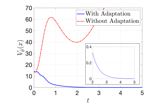
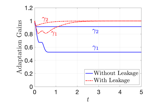
Figure 1(a) shows the uclf—an indicator of tracking performance—with and without adaptation. The proposed method (Corollary 1) successfully stabilizes the origin as predicted by Theorem 1. This is in stark contrast to the no adaptation case where only bounded error can be acheived. The uclf with leakage modification (omitted for clarity) exhibits nearly identical behavior as the uclf with the update law from Corollary 1 which confirms the result stated in Theorem 2. Figure 1(b) shows the individual adaptation gains with and without the leakage modification. The nominal case (blue) sees a reduction in the adaptations gains by 47% and 9%, respectively, indicating the adaptation transients of $\theta_{1}$ would have a large destabilizing effect if not compensated for. The leakage modification (red, $\lambda=1$ ) ensures the adaptation gains return to their nominal values as predicted by Theorem 2.

V Conclusion

We presented a new direct adaptation law that adjusts individual adaptation gains online to achieve stable closed-loop control and learning for nonlinear systems with unmatched uncertainties. A bound on the rate of change of individual adaptation gains that prevents destabilization by the adaptation transients was derived. Noteworthy extensions and modifications were also discussed. The results presented here have important implications in adaptive safety [13] and adaptive optimal control [14]. Future work will explore these implications in addition to deeper investigations into fundmanetal properties of the approach.

Appendix

Proof of Lemma 1.

Consider the time interval $t\in[t_{0},\,t_{1}]$ where $\bar{w}\triangleq{\sup}_{t\in[t_{0},\,t_{1}]}(|Kw(x(t))|)$ is the supremum of the input to Equation 4 over the time interval of interest [1]. Note the $i$ subscript is dropped for clarity. Consider the comparison system $\dot{z}=-\lambda a(z)z+a(z)\bar{w}$ where $|\rho|\leq z$ uniformly and $a(z)\triangleq 2\frac{\gamma(z)^{2}}{\nabla\gamma(z)}$ is uniformly strictly positive. The comparison system has the virtual dynamics $\dot{y}=-\lambda a(z)y+a(z)\bar{w}$ which is contracting in $y$ so any two particular solutions converge exponentially to each other [15]. Letting $\alpha(t)\triangleq\lambda\,\int_{t_{0}}^{t}a(\rho(\tau))\,d\tau>0$ , then $y(t)=y(t_{0})e^{-\alpha(t)}+\tfrac{1}{\lambda}(1-e^{-\alpha(t)})\,\bar{w}$ is the solution to the virtual dynamics and is bounded. Because $z$ is a particular solution of the virtual system and $|\rho|\leq z$ , $\rho$ is bounded. Also, as $w(x)\rightarrow 0$ then so does $\bar{w}$ over some time interval, hence $y\rightarrow 0$ and in turn $\rho\rightarrow 0$ as desired. ∎

Theorem 4 (cf. [4]).

Consider the uncertain system Equation 1 with $x_{d}$ being the desired equilibrium. If an uclf $V_{\theta}(x,t)$ exists, then, for any strictly-increasing and uniformly-positive scalar function $\upsilon(\rho)$ , $x\rightarrow x_{d}$ asymptotically with the adaptation law

	$\displaystyle\dot{\hat{\theta}}$	$\displaystyle=-\upsilon(\rho)\,\Gamma\,\Delta(x,t)\,\frac{\partial V_{\hat{\theta}}}{\partial x},$
	$\displaystyle\dot{\rho}$	$\displaystyle=-\frac{\upsilon(\rho)}{\nabla\upsilon(\rho)}\frac{1}{V_{\hat{\theta}}(x,t)+c}\frac{\partial V_{\hat{\theta}}}{\partial\hat{\theta}}^{\top}\,\dot{\hat{\theta}},$

where $\Gamma$ is a symmetric positive-definite matrix and $c\in\mathbb{R}_{>0}$ .

Acknowledgements We thank Miroslav Krstic for stimulating discussions.

References

[1] M. Krstic, P. V. Kokotovic, and I. Kanellakopoulos, Nonlinear and adaptive control design. John Wiley & Sons, 1995.
[2] E. D. Sontag and Y. Wang, “On characterizations of the input-to-state stability property,” Systems & Control Letters, vol. 24, no. 5, pp. 351–359, 1995.
[3] M. Krstić and P. V. Kokotović, “Control lyapunov functions for adaptive nonlinear stabilization,” Systems & Control Letters, vol. 26, no. 1, pp. 17–23, 1995.
[4] B. T. Lopez and J.-J. E. Slotine, “Universal adaptive control of nonlinear systems,” IEEE Control Systems Letters, vol. 6, pp. 1826–1830, 2021.
[5] W. Lohmiller and J.-J. E. Slotine, “On contraction analysis for non-linear systems,” Automatica, vol. 34, no. 6, pp. 683–696, 1998.
[6] J.-J. E. Slotine and W. Li, Applied nonlinear control. Prentice Hall, 1991.
[7] P. A. Ioannou and J. Sun, Robust adaptive control. Courier Corporation, 2012.
[8] H. Lei and W. Lin, “Universal adaptive control of nonlinear systems with unknown growth rate by output feedback,” Automatica, vol. 42, no. 10, pp. 1783–1789, 2006.
[9] Y. Song, J. Sohl-Dickstein, D. Kingma, A. Kumar, S. Ermon, and B. Poole, “Score-based generative modeling through stochastic differential equations,” ICLR, 2021.
[10] R. E. Kalman and J. E. Bertram, “Control system analysis and design via the “second method” of lyapunov: I—continuous-time systems,” Trans. ASME Basic Engineering, Ser. D, vol. 82, pp. 371–400, 1960.
[11] D. G. Luenberger, Introduction to dynamic systems; theory, models, and applications. John Wiley & Sons, 1979.
[12] J.-J. E. Slotine and W. Li, “Composite adaptive control of robot manipulators,” Automatica, vol. 25, no. 4, pp. 509–519, 1989.
[13] B. T. Lopez and J.-J. E. Slotine, “Unmatched control barrier functions: Certainty equivalence adaptive safety,” in 2023 American Control Conference (ACC), pp. 3662–3668, IEEE, 2023.
[14] B. T. Lopez and J.-J. E. Slotine, “Adaptive variants of optimal feedback policies,” in Learning for Dynamics and Control, PMLR, 2022.
[15] W. Wang and J.-J. E. Slotine, “On partial contraction analysis for coupled nonlinear oscillators,” Biological Cybernetics, vol. 92, no. 1, pp. 38–53, 2005.

Dynamic Adaptation Gains for Nonlinear Systems with Unmatched Uncertainties

Abstract

Index Terms:

I Introduction

II Problem Formulation

Assumption 1.

III Main Results

III-A Overview

III-B Unmatched Control Lyapunov Functions

Definition 1 (cf. [4]).

Remark 1.

III-C Dynamic Adaptation Gains

Definition 2.

Remark 2.

Theorem 1.

Proof.

Remark 3.

Remark 4.

Corollary 1.

Remark 5.

III-D Leakage Modification: Bounding ρ\rho

Lemma 1.

Theorem 2.

Proof.

III-E Matched and Unmatched Uncertainties

Theorem 3.

Proof.

III-F Composite Adaptation

Proposition 1.

Proof.

IV Simulation Experiments

V Conclusion

Appendix

Proof of Lemma 1.

Theorem 4 (cf. [4]).

References

III-D Leakage Modification: Bounding $\rho$