Dual-Path Cross-Modal Attention for better Audio-Visual Speech Extraction

The audio encoder is a single 1-D convolutional layer with similar structure to TasNet [1], which takes raw audio with length $T$ as input and outputs an STFT-like embedding $E_{a}\in\mathbb{R}^{T^{\prime}\times{D_{a}}}$ with feature dimension $D_{a}$ and time dimension $T^{\prime}$.

$$E_{a}=\text{conv1d}(E_{i})$$

(1)

On the visual side, we extract the face features $E_{v}\in\mathbb{R}^{T_{v}\times D_{v}}$ from video frames using a pretrained MTCNN face detection model [25] and FaceNet model [26], where $T_{v}$ denotes number of frames and $D_{v}$ is the video feature dimension.

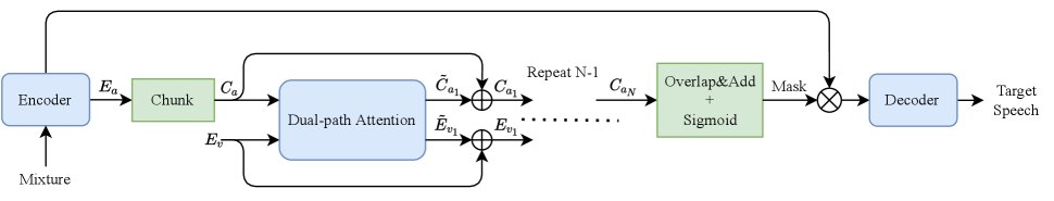
Our model is based on generating a mask on the mixture encoding. The masking network consists of a chunk operation, $N$ dual-path attention modules, an overlap and add operation to transform the chunk back to the encoding dimension, and then sigmoid activation to get the mask. The overview is shown in Figure 1A.

To prepare the audio embedding for the dual-path attention module, we follow the design of DPRNN [2] and divide $E_{a}$ into overlapping chunks with 50% overlap. By concatenating these chunks in a new time dimension, we reshape the matrix $E_{a}\in\mathbb{R}^{T^{\prime}\times D_{a}}$ into the 3-tensor $C_{a}\in\mathbb{R}^{S\times K\times D_{a}}$ where $S$ is the number of overlapping chunks and $K$ is the chunk size.

The audio 3-tensor and the visual feature matrix are then fed into $N$ connected dual-path attention modules. The dual-path attention module is covered in detail in section 2.3 below and is the main part of the masking network. Each dual-path attention module outputs two tensors which have the same dimensionality with $C_{a}$ and $E_{v}$, respectively. Residual connections are applied after each dual-path attention module. Each module’s output is fed as input to the next module, until all $N$ modules are all applied. Assume $C_{a_{i}}$ and $E_{v_{i}}$ are the outputs of the $i^{\textrm{th}}$ dual-path attention module and $C_{a_{0}}=C_{a},E_{v_{0}}=E_{v}$, then for $i\in[1,N]$ we have:

	$\displaystyle\tilde{C}_{a_{i}},\tilde{E}_{v_{i}}\leftarrow\text{DualPathAttention}(C_{a_{i-1}},E_{v_{i-1}})$		(2)
	$\displaystyle C_{a_{i}}\!=\!\text{LN}\left(\tilde{C}_{a_{i}}\!+C_{a_{i-1}}\right),\;\;E_{v_{i}}\!=\!\text{LN}\left(\tilde{E}_{v_{i}}\!+E_{v_{i-1}}\right)$		(3)

After $N$ dual-path attention modules, the 50% overlap-add operation is applied to transform the 3-tensor to a 2-D encoding with the same dimension as the audio encoder output. The 2-D encoding is passed through a sigmoid to get a mask; the Hadamard product of the mask and the audio encoder output is the encoding of the target speech.

Each dual-path attention module consists of $N_{\textrm{intra}}$ intra-chunk modules, followed by $N_{\textrm{inter}}$ inter-chunk attention modules, as shown in Fig. 2. Each dual-path attention module begins (at the bottom of Fig. 2) by passing the audio features $C_{a_{i}}$ through $N_{\textrm{intra}}$ consecutive intra-chunk attention modules. Then the extracted local features are fed into the inter-chunk attention module to model long-term temporal structure and audio-visual correspondence. Residual connections after each intra-chunk and inter-chunk module improve convergence.

The intra-chunk attention module aims to learn local temporal structure of the chunked audio feature. It consists of $N_{intra}$ layers, where each layer takes the chunked audio feature $C_{a}\in\mathbb{R}^{S\times K\times D_{a}}$ as input and outputs a tensor with the same size. Inside each layer, a MultiHeadAttention (MHA) and a position-wise feedforward layer are applied to each of the $S$ chunks separately, while residual addition and LayerNorm (LN) are applied after both MHA and FeedForward, so for all $s\in[1,S]$:

	$\displaystyle C_{a}[s,:,:]$	$\displaystyle\leftarrow\text{LN}(C_{a}[s,:,:]+\text{MHA}(C_{a}[s,:,:]))$		(4)
	$\displaystyle C_{a}[s,:,:]$	$\displaystyle\leftarrow\text{LN}(C_{a}[s,:,:]+\text{FeedForward}(C_{a}[s,:,:]))$		(5)

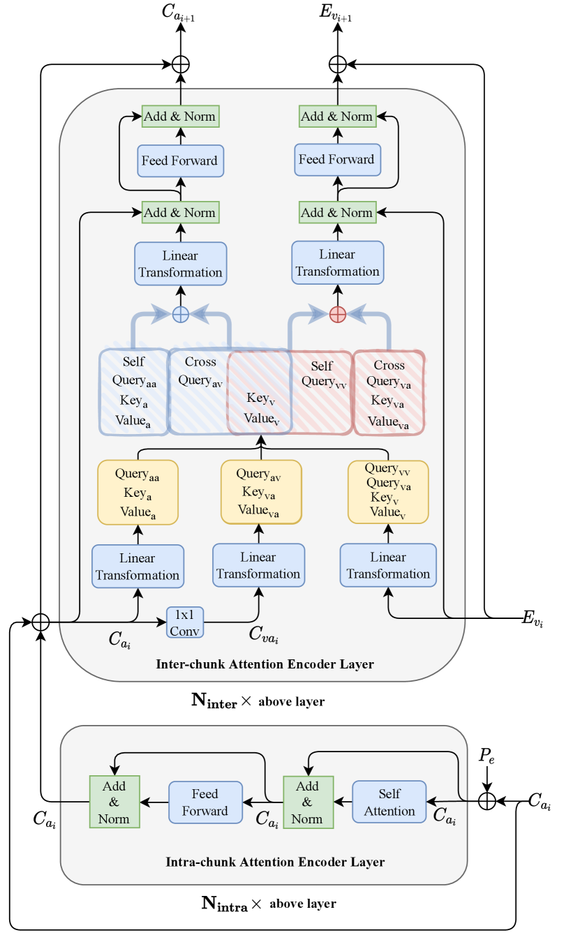
The inter-chunk attention module aims to deal with long-term audio-visual information. Similar to the intra-chunk attention module, each inter-chunk attention module has $N_{inter}$ encoder layers. However, different from the intra-chunk attention module, each layer in the inter-chunk attention module receives audio chunked features $C_{a}\in\mathbb{R}^{S\times K\times D_{a}}$ and visual features $E_{v}\in\mathbb{R}^{S\times D_{v}}$ as input, and then applies both self-attention for each modality and cross-attention between modalities. This makes sure that each modality can attend to both itself and the other modality, which allows both information fusion and learning long-term temporal structures.

Self-attention for the visual information $E_{v}\in\mathbb{R}^{S\times D_{v}}$ is a simple attention module as proposed in the original transformer paper [27]. $\text{query}_{vv}$, $\text{key}_{v}$, and $\text{value}_{v}$ with dimension $\mathbb{R}^{S\times(h\times D_{k})}$ are generated from linear transformations on $E_{v}$, where $S$ is the time dimension, $D_{v}$ is the visual feature dimension, $h$ is the number of heads, and $D_{k}$ is the internal dimension for each head. In the following formulas, linear transformation is abbreviated as LT.

	$\displaystyle\text{query}_{vv},\text{key}_{v},\text{value}_{v}=LT_{D_{v}\rightarrow(h\times D_{k})}(E_{v})$		(6)
	$\displaystyle x_{vv}=\text{Attention}(\text{query}_{vv},\text{key}_{v},\text{value}_{v})$		(7)

Self-attention for the chunked audio features $C_{a}\in\mathbb{R}^{S\times K\times D_{a}}$ is similar to the visual side, but with an extra K dimension. We just do multihead-attention for each slice on the K dimension $C_{a_{k}}\in\mathbb{R}^{S\times D_{a}}$ and concatenate the results.

	$\displaystyle\text{query}_{aa_{k}},\text{key}_{a_{k}},\text{value}_{a_{k}}=LT_{D_{a}\rightarrow(h\times D_{k})}(C_{a}[:,k,:])$		(8)
	$\displaystyle x_{aa}[:,k,:]=\text{Attention}(\text{query}_{aa_{k}},\text{key}_{a_{k}},\text{value}_{a_{k}})$		(9)

For cross-attention between modalities, although the chunking step helps us match the long-term time dimension with size $S$ for the video and audio input, the audio input still has an extra short-term dimension with size $K$(chunk size) compared to the video input. We find that doing cross-attention between each slice of the audio chunked features and the video features requires a large amount of computation and does not provide a significant performance gain. That’s because for attention computation with long-term information, the attention computation is similar for each audio feature slice $C_{a}[:,k,:]$. So to do cross-attention efficiently, we choose to collapse the $K$ dimension of the audio features by a single $1\times 1$ convolutional operation and use the collapsed audio feature $C_{va}\in\mathbb{R}^{S\times D_{a}}$ as the audio modality for cross-attention.

	$\displaystyle C_{va}[s,d]=1\times 1\hskip 3.01125pt\text{Conv}(C_{a}[s,:,d])$		(10)
	$\displaystyle\text{query}_{va}=LT_{D_{v}\rightarrow(h\times D_{k})}(E_{v})$		(11)
	$\displaystyle\text{query}_{av},\text{key}_{va},\text{value}_{va}=LT_{D_{a}\rightarrow(h\times D_{k})}(C_{va})$		(12)

All the keys, values, and queries used in cross-attention have the same dimension $\mathbb{R}^{S\times(h\times D_{k})}$, so the cross-attention computation is just a simple attention computation similar to the one in the visual information self-attention step:

	$\displaystyle x_{av}=\text{Attention}(\text{query}_{av},\text{key}_{v},\text{value}_{v})$		(13)
	$\displaystyle x_{va}=\text{Attention}(\text{query}_{va},\text{key}_{va},\text{value}_{va})$		(14)

We add self-attention result and cross-attention result for each modality. On the visual side, $x_{vv}$ and $x_{va}$ have the same dimension $\mathbb{R}^{S\times(h\times D_{k})}$, so simple element-wise addition works. On the audio side where the self-attention result $x_{aa}$ has an additional K (Chunk Size) dimension, we need to broadcast $x_{av}$ in this dimension so that the result of addition has dimension $\mathbb{R}^{S\times K\times(h\times D_{k})}$. Then we use a linear transformation, followed by LayerNorm, followed by a two-layer feedforward network (FF), to turn the audio and video embeddings with features dimension of $(h\times D_{k})$ back into $D_{a}$ and $D_{v}$ respectively:

	$\displaystyle\tilde{C}_{a_{i}}=\text{FF}\left(\text{LN}(C_{a_{i-1}}+LT_{(h\times D_{k})\rightarrow D_{a}}(x_{aa}+x_{av}))\right)$		(15)
	$\displaystyle\tilde{E}_{v_{i}}=\text{FF}\left(LN(E_{v_{i-1}}+LT_{(h\times D_{k})\rightarrow D_{v}}(x_{vv}+x_{va}))\right)$		(16)

$\tilde{C}_{a_{i}}$ and $\tilde{E}_{v_{i}}$ are then augmented by another residual connection and another LayerNorm, as shown in Eq. (3).

Overlap-add with 50% overlap transforms the chunked audio features with dimension $\mathbb{R}^{S\times K\times D_{a}}$ back into $\mathbb{R}^{T^{\prime}\times D_{a}}$, which then masks the mixture encoding, as described in Section 2.2. Finally, the masked audio features are fed into the decoder which is a transposed convolutional layer to output the separated audio. Below $\odot$ represents Hadamard product.

	$\displaystyle M=\text{Sigmoid}(\text{Overlap\&Add}(C_{a_{N}}))$		(17)
	$\displaystyle x_{extracted}=\text{TransposedConv1d}(M\odot E_{a})$		(18)

Hyperparameters are set as follows: $N=3$, $N_{intra}=4$, $N_{inter}=4$, $K=160$, $D_{a}=256$, $D_{v}=512$. In the video processing stage, MTCNN extracts a 160$\times$160 patch for each image frame. The pretrained FaceNet model then further processes the video frames and turns each frame into a feature embedding with 512 dimensions. On the audio side, the audio encoder has a window size of 16, stride of 8, and output dimension of 256. Cropped facial regions are then fed together with audio features into the sequence of $N=3$ dual-path attention modules, each of which contains $N_{intra}=4$ intra-chunk and $N_{inter}=4$ inter-chunk attention modules.

The configuration of multi-headed attention is the same for both intra-chunk and inter-chunk modules, each with $h=8$ heads of internal dimension $D_{k}=64$. After the attention calculation, linear layers are applied to the attention output with respectively 256 dimensions for audio and 512 dimensions for video. The FeedForward layer is just two linear layers with the intermediate feature dimension $D_{f}=1024$. For pretraining process with the GRID dataset [28], the attention field covers the entire sequence. For later training and validation with the LRS3 dataset where each utterance has an 8-second duration, we apply a mask during attention calculation to limit the attention field to a 5 second duration around the current timestep.

Our final evaluation of the audio-visual model is done on the LRS3 dataset [29]. However, we notice that LRS3 is a difficult task for the audio-visual model for three reasons. First, the video channel of LRS3 is not ideal: many image frames are non-frontal faces, and some miss the face entirely. Second, the audio channel of LRS3 has significant reverberation which makes it harder to separate out the original audio. Third, the number of speakers in LRS3 is very large, therefore it is rare for the same speaker to be repeated from one batch to the next, which makes it harder for the network to acquire useful gradients during the initial training phase.

We therefore choose to pretrain our model on the GRID corpus [28], a smaller and easier dataset, before moving on to LRS3. The GRID corpus consists of 33 speakers (one speaker missing) where each speaker has 1000 3-second long utterances of simple sentences and video capturing the frontal face area. We pretrain on GRID for 10 epochs with the same training configurations mentioned below before moving to LRS3 dataset.

For the LRS3 dataset, we choose a subset of 33,000 utterances out of the whole LRS3 dataset and clip the audio and video to be 8 seconds per utterance, with a 16 kHz audio sampling rate and 25 video frames per second. From the 33000 extracted utterances, we use 27000 utterances for training, 3000 for validation, and 3000 for testing. Thus we have 60 hours of LRS3 training data, 6.67 hours for validation, and 6.67 hours for testing. The LibriSpeech and LibriMix datasets [30, 31] are used as interference speech with non-overlapping train/validation/test split. For each training sample, we randomly assign 1-4 interference speakers. The SI-SNR for the mixture is synthesized with SI-SNR (dB) drawn randomly from $\text{Uniform}(\mu-5,\mu+5)$ where $\mu$ is predefined according to the number of interference speakers. We set $\mu=0,-3.4,-5.4,-6.7$ for $1,2,3,4$ interference speakers, respectively. For the testing set, we have the exact same configuration.

Empirically, we find that including 1-4 interfering speakers during training helps the model to improve performance on the validation set even when the validation set has only 2 speakers/mixture. Specifically, this approach helps the model to tackle difficult cases where the voice features of the target speaker and the interference speaker are similar. In these bad samples, the model is likely to make wrong choices determining the target speaker, so that even if the model is able to separate the speakers perfectly, the output is completely wrong. Including more interference speakers helps the model learn how to discriminate the target speaker from the others and thus improve the validation performance.

We use SI-SNR [32] as the training objective. We use Adam optimizer [33] with initial learning rate 1e-4. We decay the learning rate by a factor of 2 when the validation SI-SNR stops improving for three consecutive epochs. The whole training process is in mixed precision with batch size 1 on one single V100 GPU. The entire training process lasts for 50 epochs.

References

- [1] Y. Luo and N. Mesgarani, “Conv-tasnet: Surpassing ideal time–frequency magnitude masking for speech separation,” IEEE/ACM Transactions on Audio, Speech, and Language Processing, vol. 27, no. 8, p. 1256–1266, Aug 2019. [Online]. Available: http://dx.doi.org/10.1109/TASLP.2019.2915167
- [2] Y. Luo, Z. Chen, and T. Yoshioka, “Dual-path rnn: efficient long sequence modeling for time-domain single-channel speech separation,” 2020.
- [3] C. Subakan, M. Ravanelli, S. Cornell, M. Bronzi, and J. Zhong, “Attention is all you need in speech separation,” 2021.
- [4] E. Nachmani, Y. Adi, and L. Wolf, “Voice separation with an unknown number of multiple speakers,” 2020.
- [5] J. Chen, Q. Mao, and D. Liu, “Dual-path transformer network: Direct context-aware modeling for end-to-end monaural speech separation,” arXiv preprint arXiv:2007.13975, 2020.
- [6] H. McGurk and J. MacDonald, “Hearing lips and seeing voices,” Nature, vol. 264, no. 5588, pp. 746–748, 1976.
- [7] J. S. Chung, A. Senior, O. Vinyals, and A. Zisserman, “Lip reading sentences in the wild,” 2017 IEEE Conference on Computer Vision and Pattern Recognition (CVPR), Jul 2017. [Online]. Available: http://dx.doi.org/10.1109/CVPR.2017.367
- [8] T. Afouras, J. S. Chung, A. Senior, O. Vinyals, and A. Zisserman, “Deep audio-visual speech recognition,” IEEE Transactions on Pattern Analysis and Machine Intelligence, p. 1–1, 2019. [Online]. Available: http://dx.doi.org/10.1109/TPAMI.2018.2889052
- [9] B. Shi, W.-N. Hsu, K. Lakhotia, and A. Mohamed, “Learning audio-visual speech representation by masked multimodal cluster prediction,” in International Conference on Learning Representations, 2022. [Online]. Available: https://openreview.net/forum?id=Z1Qlm11uOM
- [10] P. Ma, S. Petridis, and M. Pantic, “End-to-end audio-visual speech recognition with conformers,” ICASSP 2021 - 2021 IEEE International Conference on Acoustics, Speech and Signal Processing (ICASSP), pp. 7613–7617, 2021.
- [11] B. Garcia, B. Shillingford, H. Liao, O. Siohan, O. de Pinho Forin Braga, T. Makino, and Y. Assael, “Recurrent neural network transducer for audio-visual speech recognition,” in Proceedings of IEEE Automatic Speech Recognition and Understanding Workshop, 2019. [Online]. Available: https://arxiv.org/abs/1911.04890
- [12] G. Sterpu, C. Saam, and N. Harte, “Attention-based audio-visual fusion for robust automatic speech recognition,” in Proceedings of the 20th ACM International Conference on Multimodal Interaction, 2018, pp. 111–115.
- [13] H. Wang, F. Gao, Y. Zhao, and L. Wu, “Wavenet with cross-attention for audiovisual speech recognition,” IEEE Access, vol. 8, pp. 169 160–169 168, 2020.
- [14] A. Nagrani, S. Yang, A. Arnab, A. Jansen, C. Schmid, and C. Sun, “Attention bottlenecks for multimodal fusion,” 2022.
- [15] H. Akbari, H. Arora, L. Cao, and N. Mesgarani, “Lip2audspec: Speech reconstruction from silent lip movements video,” CoRR, vol. abs/1710.09798, 2017. [Online]. Available: http://arxiv.org/abs/1710.09798
- [16] A. Ephrat and S. Peleg, “Vid2speech: speech reconstruction from silent video,” in 2017 IEEE International Conference on Acoustics, Speech and Signal Processing (ICASSP). IEEE, 2017.
- [17] K. R. Prajwal, R. Mukhopadhyay, V. Namboodiri, and C. V. Jawahar, “Learning individual speaking styles for accurate lip to speech synthesis,” CoRR, vol. abs/2005.08209, 2020. [Online]. Available: https://arxiv.org/abs/2005.08209
- [18] T. Afouras, J. S. Chung, and A. Zisserman, “The conversation: Deep audio-visual speech enhancement,” 2018.
- [19] ——, “My lips are concealed: Audio-visual speech enhancement through obstructions,” 2019.
- [20] J. Wu, Y. Xu, S.-X. Zhang, L.-W. Chen, M. Yu, L. Xie, and D. Yu, “Time domain audio visual speech separation,” 2019.
- [21] H. Sato, T. Ochiai, K. Kinoshita, M. Delcroix, T. Nakatani, and S. Araki, “Multimodal attention fusion for target speaker extraction,” 2021.
- [22] A. Gabbay, A. Shamir, and S. Peleg, “Visual speech enhancement,” 2018.
- [23] Y. Luo, J. Wang, L. Xu, and L. Yang, “Multi-Stream Gated and Pyramidal Temporal Convolutional Neural Networks for Audio-Visual Speech Separation in Multi-Talker Environments,” in Proc. Interspeech 2021, 2021, pp. 1104–1108.
- [24] A. Ephrat, I. Mosseri, O. Lang, T. Dekel, K. Wilson, A. Hassidim, W. T. Freeman, and M. Rubinstein, “Looking to listen at the cocktail party,” ACM Transactions on Graphics, vol. 37, no. 4, p. 1–11, Aug 2018. [Online]. Available: http://dx.doi.org/10.1145/3197517.3201357
- [25] K. Zhang, Z. Zhang, Z. Li, and Y. Qiao, “Joint face detection and alignment using multitask cascaded convolutional networks,” IEEE Signal Processing Letters, vol. 23, no. 10, p. 1499–1503, Oct 2016. [Online]. Available: http://dx.doi.org/10.1109/LSP.2016.2603342
- [26] F. Schroff, D. Kalenichenko, and J. Philbin, “Facenet: A unified embedding for face recognition and clustering,” 2015 IEEE Conference on Computer Vision and Pattern Recognition (CVPR), Jun 2015. [Online]. Available: http://dx.doi.org/10.1109/CVPR.2015.7298682
- [27] A. Vaswani, N. Shazeer, N. Parmar, J. Uszkoreit, L. Jones, A. N. Gomez, L. Kaiser, and I. Polosukhin, “Attention is all you need,” CoRR, vol. abs/1706.03762, 2017. [Online]. Available: http://arxiv.org/abs/1706.03762
- [28] M. Cooke, J. Barker, S. Cunningham, and X. Shao, “An audio-visual corpus for speech perception and automatic speech recognition,” The Journal of the Acoustical Society of America, vol. 120, no. 5, pp. 2421–2424, 2006. [Online]. Available: https://doi.org/10.1121/1.2229005
- [29] T. Afouras, J. S. Chung, and A. Zisserman, “Lrs3-ted: a large-scale dataset for visual speech recognition,” in arXiv preprint arXiv:1809.00496, 2018.
- [30] V. Panayotov, G. Chen, D. Povey, and S. Khudanpur, “Librispeech: An asr corpus based on public domain audio books,” in 2015 IEEE International Conference on Acoustics, Speech and Signal Processing (ICASSP), 2015, pp. 5206–5210.
- [31] J. Cosentino, M. Pariente, S. Cornell, A. Deleforge, and E. Vincent, “Librimix: An open-source dataset for generalizable speech separation,” arXiv preprint arXiv:2005.11262, 2020.
- [32] J. Le Roux, S. Wisdom, H. Erdogan, and J. R. Hershey, “Sdr–half-baked or well done?” in ICASSP 2019-2019 IEEE International Conference on Acoustics, Speech and Signal Processing (ICASSP). IEEE, 2019, pp. 626–630.
- [33] D. P. Kingma and J. Ba, “Adam: A method for stochastic optimization,” 2017.
- [34] M. Kolbæk, D. Yu, Z.-H. Tan, and J. Jensen, “Multi-talker speech separation with utterance-level permutation invariant training of deep recurrent neural networks,” 2017.