DTR: A Unified Deep Tensor Representation Framework for Multimedia Data Recovery
Abstract
Recently, the transform-based tensor representation has attracted increasing attention in multimedia data (e.g., images and videos) recovery problems, which consists of two indispensable components, i.e., transform and characterization. Previously, the development of transform-based tensor representation mainly focuses on the transform aspect. Although several attempts consider using shallow matrix factorization (e.g., singular value decomposition and negative matrix factorization) to characterize the frontal slices of transformed tensor (termed as latent tensor), the faithful characterization aspect is underexplored. To address this issue, we propose a unified Deep Tensor Representation (termed as DTR) framework by synergistically combining the deep latent generative module and the deep transform module. Especially, the deep latent generative module can faithfully generate the latent tensor as compared with shallow matrix factorization. The new DTR framework not only allows us to better understand the classic shallow representations, but also leads us to explore new representation. To examine the representation ability of the proposed DTR, we consider the representative multi-dimensional data recovery task and suggest an unsupervised DTR-based multi-dimensional data recovery model. Extensive experiments demonstrate that DTR achieves superior performance compared to state-of-the-art methods in both quantitative and qualitative aspects, especially for fine details recovery.
Index Terms:
Deep tensor representation, deep latent generative module, deep transform module, multi-dimensional data recovery.I Introduction
Multimedia data, such as color images [1, 2, 3], multispectral images (MSIs) [4, 5], magnetic resonance imaging (MRI) images [6], and videos [7, 8], is commonly encountered in various real-world applications, including but not limited to agricultural monitoring [9], hyperspectral image (HSI) restoration [10, 11], and medical imaging [12]. However, the acquired multimedia data is usually incomplete owing to sensor failures or other abnormal conditions that occur during the acquisition and transmission process, which can severely hinder subsequent applications [13, 14, 15]. The task of estimating missing data from the observed data can be formulated as the multimedia data recovery problem. Besides, with the development of multimedia technology, multimedia data has become increasingly multi-dimensional. Hence, it is important to develop effective multi-dimensional data recovery methods.


Recently, the transform-based tensor representation has emerged as a powerful tool for multi-dimensional data recovery problems, as demonstrated by extensive studies [18, 19, 17, 20, 21, 22]. The transform-based tensor representation represents the multi-dimensional data as an implicit low-rank tensor and exploits its low-rankness in the transform domain. In the transform-based tensor representation, two indispensable components are (i) the transform that captures the frontal slice relationships of multi-dimensional data [20, 21, 22], and (ii) the characterization of the frontal slices of transformed tensor (termed as latent tensor) [23, 24, 25].
Previously, the development of transform-based tensor representation mainly focuses on the transform perspective, such as the discrete Fourier transform (DFT) [23, 26], the discrete cosine transform (DCT) [22], unitary transform [27, 28], non-invertible transform [20, 29, 30], and nonlinear transform [17]. However, few methods have paid attention to the second component, i.e., the characterization of the frontal slices of latent tensor. To date, the transform-based tensor representation usually adopts shallow matrix factorization to characterize the frontal slices of latent tensor, such as singular value decomposition (SVD) [23], negative matrix factorization (NMF) [17, 24], and QR decomposition [31, 25]. Due to the limited characterization ability, these shallow methods may not be expressive enough to faithfully characterize the latent tensor. Moreover, shallow matrix factorization characterizes the intra-slice relationships of latent tensor separately, which neglects the inter-slice relationships of latent tensor.
To address the above issues, we propose a unified Deep Tensor Representation (termed as DTR) framework by synergistically combining the deep latent generative module and the deep transform module. Specifically, we suggest a deep latent generative module to faithfully generate the latent tensor by characterizing both intra-slice and inter-slice relationships of latent tensor. Meanwhile, we utilize an untrained neural network applied on the third dimension of latent tensor as the deep transform module to capture the frontal slice relationships of multi-dimensional data. The new DTR framework not only allows us to better understand the classic shallow representations, but also leads us to explore new representation. To examine the representation ability of the proposed DTR, we consider the representative multi-dimensional data recovery task and suggest an unsupervised DTR-based multi-dimensional data recovery model. Thanks to the superior characterization ability of deep latent generator, our method can obtain better multi-dimensional data recovery results than shallow characterization-based methods; as shown in Fig. 1.
The main contributions of this study are:
-
•
To overcome the limitations of shallow characterization in the transform-based tensor representation, we propose a unified deep tensor representation framework, i.e., DTR, by synergistically combining the deep latent generative module and the deep transform module. The new DTR framework not only allows us to better understand the classic shallow representations, but also leads us to explore new representation.
-
•
Based on the DTR, we propose an unsupervised multi-dimensional data recovery model. Experimental results demonstrate that the proposed method can achieve significant performance improvements over state-of-the-art methods, especially for fine details recovery.
This paper is organized as follows. Section II introduces necessary notations and preliminaries. Section III provides a review of related work. Section IV presents the proposed DTR. Section V and VI present the results of extensive experiments and discussions. Finally, we conclude this work in Section VII.
II Notations and preliminaries
II-A Notations
Matrices and tensors are denoted by capitalized letters, e.g., and capitalized calligraphic letters, e.g., , respectively. For a matrix , we use to denote the -th element of . Meanwhile, for a third-order tensor , we use to denote the -th element of . denotes the -th frontal slice of . denotes the point-wise multiplication (i.e., Hadamard product). The Frobenius norm of tensor is defined as . denotes the face-wise product between two tensors [32]. Given , , the face-wise product between and is , where .
II-B Preliminaries
Definition 1 (Mode-3 Unfolding [33]).
For a third-order tensor , its mode- unfolding is a matrix, which satisfies that , where with .
Definition 2 (Mode-3 Tensor-Matrix Product [33]).
The mode-3 tensor-matrix product of a tensor and a matrix is a tensor denoted by and satisfied
| (1) |
According to above mentioned two definitions, we have
| (2) |
Definition 3 (Tensor Tubal-Rank [32]).
The tensor tubal-rank of is defined as
| (3) |
where is the DFT matrix.
Definition 4 (T-Product [32]).
The tensor-tensor product between , and is defined as , where is the DFT matrix, and is the inverse DFT matrix.
III Related work
In this section, we briefly review the transform-based tensor representation, with a focus on the advances of two indispensable components, i.e., transform and characterization.
III-A The Transform Perspective
An indispensable component in the transform-based tensor representation is the transform that captures the frontal slice relationships of multi-dimensional data. Over the past decade, researchers have explored various transforms [22, 28, 20, 30, 17] to facilitate the most classic transform-based tensor representation, i.e., tensor singular value decomposition (t-SVD). For instance, Kilmer et al. [23] first introduced the DFT along the third dimension under the t-SVD framework. Madathil et al. [22] adopted the real-valued DCT to avoid the high computational cost caused by complex operations in DFT-based original t-SVD. Lu et al. [21] deduced the new tensor tubal rank based on the invertible linear transform and provided the theoretical bound for the exact recovery under certain tensor incoherence conditions for tensor completion. Unlike previous invertible transforms, Jiang et al. [20] employed the non-invertible framelet transform to construct a framelet latent tensor. In addition to the previously pre-defined transforms, some data-driven transforms have emerged promising results in multi-dimensional data recovery problems. For example, Song et al. [28] constructed a data-dependent unitary transform, which can be obtained by taking the SVD of the unfolding matrix. Kong et al. [30] defined the new tensor Q-rank based on novel data-dependent transform, which can be learned by principal component analysis. Luo et al. [34] proposed a nonlinear transform-based tensor nuclear norm (TNN), where the nonlinear transform is obtained by learning a multi-layer neural network solely using the observed tensor in a self-supervised manner.
III-B The Characterization Perspective
Another indispensable component in the transform-based tensor representation is the characterization of the frontal slices of latent tensor. The original t-SVD [23] adopted the standard matrix SVD to characterize the frontal slices of latent tensor. Zhou et al. [24] introduced NMF as an alternative approach to efficiently characterize the low-rankness of the frontal slices of latent tensor. In addition, to further enhance the accuracy and efficiency of the characterization, later work [31, 25] adopted an approximate SVD method based on QR decomposition to characterize the frontal slices of latent tensor, which not only reduces the computational complexity but also yields superior results compared to SVD-based method [16]. Despite the benefits of shallow matrix factorization (such as SVD, NMF, and QR decomposition), they may not be representative enough to characterize the latent tensor. Moreover, shallow matrix factorization characterizes the intra-slice relationships of latent tensor separately, which neglects the inter-slice relationships of latent tensor.
IV Proposed method
In this section, we first introduce the proposed unified deep tensor representation framework, i.e., DTR. Then, we discuss the relationships between the proposed DTR and classic shallow representations. Finally, we give the unsupervised DTR-based multi-dimensional data recovery model.
IV-A The Proposed DTR
Inspired by the transform-based tensor representation, we propose a unified deep tensor representation framework, i.e., DTR, by synergistically combining the deep latent generative module and the deep transform module. The diagram of our DTR framework is shown in Fig. 1, and the mathematical formulation can be expressed as follows:
| (4) |
where is the deep latent generative module, denotes the network parameter of , and is a random noise. is the deep transform module, denotes the network parameter of , denotes the composition of functions, and is the multi-dimensional data represented by the proposed DTR. Two indispensable components in the proposed DTR framework, i.e., the deep latent generative module and the deep transform module , complement to each other and work together to make up a unified framework. Now, we detailedly introduce the two indispensable components in our DTR framework.
IV-A1 Deep Latent Generative Module
Previous representation usually adopts shallow matrix factorization to characterize the intra-slice relationships of latent tensor separately, which neglects the inter-slice relationships of latent tensor. In our DTR framework, we suggest the deep latent generative module to generate the latent tensor, which can be formulated as follows:
| (5) |
where : , denotes the network parameter of , is a random noise, and represents the latent tensor. Here, refers to an untrained neural network that maps a random noise into the latent tensor.
Compared with shallow matrix factorization (e.g., SVD and NMF), the deep latent generator can faithfully generate the latent tensor due to the strong representation ability of untrained neural network. In addition, the deep latent generator can faithfully characterize both intra-slice and inter-slice relationships of latent tensor. Based on these two advantages, the deep latent generator has superior characterization ability than shallow matrix factorization, rationally leading to better performance for recovering the fine details of multi-dimensional data (see examples in Fig. 1).
IV-A2 Deep Transform Module
Now, we are at the position to generate the multi-dimensional data from the latent tensor. To better capture the frontal slice relationships of multi-dimensional data, we utilize an untrained neural network applied on the third dimension of latent tensor as the deep transform module, i.e.,
| (6) |
where : , denotes the network parameter of , is the output of , i.e., the latent tensor, and is the multi-dimensional data represented by the proposed DTR. Here, maps the latent tensor into the original domain to capture the frontal slice relationships of multi-dimensional data.
The proposed DTR framework allows us to more deeply understand existing representations. Now, we discuss the relationships between the proposed DTR and classic shallow representations.
Remark 1.
Let (with , ). Suppose that is given as follows:
| (7) |
where each frontal slice of is set as an identity matrix, denotes the face-wise product between two tensors [32], and is a nonlinear activation function. The proposed DTR can degenerate into classic shallow representations:
(i) When and is set as a identity mapping, our DTR degenerates into the deep matrix factorization [35, 36], which is applied on each frontal slice of the tensor separately.
(ii) When and is set as a deep fully connected network (FCN), our DTR degenerates into the hierarchical low-rank tensor factorization [17].
(iii) When and is set as an inverse DFT, our DTR degenerates into the classic low-tubal-rank tensor factorization [24].

Moreover, the proposed DTR framework also allows us to explore new representation. Previously, the faithful characterization aspect is underexplored. Several attempts consider using shallow matrix factorization (e.g., SVD and NMF) in the transform-based tensor representation to characterize the intra-slice relationships of latent tensor separately, which neglects the inter-slice relationships of latent tensor. To faithfully characterize both intra-slice and inter-slice relationships of latent tensor, we can generate the latent tensor with an untrained neural network by leveraging its expressive power under the DTR framework; see Fig. 1 for the comparison between shallow characterizations and deep characterization in the DTR.
IV-B Unsupervised Multi-Dimensional Data Recovery Model
To examine the representation ability of the proposed DTR, we consider the representative multi-dimensional data recovery task and suggest an unsupervised DTR-based multi-dimensional data recovery model, as follow:
| (8) |
Here, is the observed multi-dimensional data, is the multi-dimensional data represented by the proposed DTR, is a binary mask tensor that sets the observed location to be ones and others be zeros, is the deep latent generative module, and is the deep transform module.
Although the model (8) is highly non-convex and nonlinear, there are still numerous available methods that can solve it. Specifically, we consider using the popular gradient descent optimization algorithm in deep learning, i.e., the adaptive moment estimation (Adam) [37] algorithm, to effectively optimize and . Once the optimal and are obtained, the multi-dimensional data can be achieved by Eq. (4).
| Method | TNN [16] | TRLRF [38] | FTNN [20] | FCTN [39] | HLRTF [17] | DTR | |||||||
|---|---|---|---|---|---|---|---|---|---|---|---|---|---|
| Data | Sampling rate | PSNR | SSIM | PSNR | SSIM | PSNR | SSIM | PSNR | SSIM | PSNR | SSIM | PSNR | SSIM |
| HSI | 0.1 | 33.56 | 0.9176 | 25.86 | 0.6817 | 37.71 | 0.9634 | 38.72 | 0.9487 | 40.88 | 0.9839 | 45.05 | 0.9932 |
| WDC | 0.2 | 38.20 | 0.9668 | 26.49 | 0.7134 | 43.87 | 0.9879 | 43.59 | 0.9893 | 43.54 | 0.9906 | 47.08 | 0.9954 |
| (256256191) | 0.3 | 41.47 | 0.9827 | 28.72 | 0.7971 | 47.60 | 0.9938 | 44.72 | 0.9916 | 45.81 | 0.9941 | 47.86 | 0.9959 |
| HSI | 0.1 | 32.70 | 0.8989 | 30.74 | 0.8439 | 38.00 | 0.9705 | 39.05 | 0.9692 | 41.71 | 0.9845 | 45.87 | 0.9942 |
| Pavia | 0.2 | 37.86 | 0.9610 | 32.05 | 0.8771 | 44.78 | 0.9921 | 46.74 | 0.9941 | 46.75 | 0.9948 | 49.32 | 0.9968 |
| (25625680) | 0.3 | 41.57 | 0.9809 | 34.14 | 0.9170 | 48.80 | 0.9963 | 48.28 | 0.9958 | 49.09 | 0.9968 | 50.22 | 0.9974 |
| MSI | 0.1 | 23.41 | 0.6456 | 23.13 | 0.5738 | 25.36 | 0.7818 | 26.26 | 0.7101 | 30.41 | 0.8983 | 33.38 | 0.9582 |
| Beads | 0.2 | 28.05 | 0.8330 | 26.63 | 0.7316 | 30.96 | 0.9196 | 31.84 | 0.8906 | 36.88 | 0.9736 | 39.03 | 0.9872 |
| (25625631) | 0.3 | 31.82 | 0.9165 | 27.68 | 0.7742 | 35.17 | 0.9647 | 38.01 | 0.9671 | 41.30 | 0.9905 | 43.89 | 0.9950 |
| MSI | 0.1 | 25.17 | 0.7853 | 24.34 | 0.7225 | 28.45 | 0.8995 | 27.39 | 0.8455 | 31.54 | 0.9430 | 32.34 | 0.9643 |
| Cloth | 0.2 | 29.73 | 0.9110 | 27.69 | 0.8473 | 33.54 | 0.9666 | 33.51 | 0.9569 | 38.12 | 0.9861 | 39.76 | 0.9921 |
| (25625631) | 0.3 | 33.36 | 0.9577 | 28.72 | 0.8733 | 37.31 | 0.9855 | 36.72 | 0.9667 | 42.56 | 0.9947 | 43.26 | 0.9957 |
| MSI | 0.1 | 31.94 | 0.7925 | 21.75 | 0.4215 | 35.96 | 0.8821 | 32.46 | 0.7666 | 40.45 | 0.9362 | 40.81 | 0.9445 |
| Flowers | 0.2 | 35.97 | 0.8660 | 26.01 | 0.5419 | 40.60 | 0.9230 | 38.85 | 0.8753 | 44.96 | 0.9521 | 45.95 | 0.9698 |
| (25625631) | 0.3 | 38.66 | 0.8948 | 27.00 | 0.6326 | 43.53 | 0.9377 | 39.94 | 0.8922 | 48.33 | 0.9714 | 48.34 | 0.9728 |
| MSI | 0.1 | 30.01 | 0.9113 | 31.01 | 0.8662 | 31.40 | 0.9657 | 29.23 | 0.8713 | 31.91 | 0.9596 | 33.95 | 0.9615 |
| Cd | 0.2 | 33.81 | 0.9537 | 34.35 | 0.9316 | 35.85 | 0.9843 | 36.58 | 0.9510 | 36.55 | 0.9836 | 39.17 | 0.9839 |
| (25625631) | 0.3 | 36.93 | 0.9729 | 35.98 | 0.9491 | 38.78 | 0.9901 | 38.39 | 0.9640 | 38.61 | 0.9884 | 41.46 | 0.9887 |
| MSI | 0.1 | 37.88 | 0.9679 | 37.94 | 0.9650 | 41.54 | 0.9871 | 40.65 | 0.9702 | 43.80 | 0.9890 | 43.83 | 0.9882 |
| Beers | 0.2 | 43.50 | 0.9902 | 40.75 | 0.9782 | 47.13 | 0.9957 | 44.84 | 0.9878 | 47.93 | 0.9948 | 48.71 | 0.9958 |
| (25625631) | 0.3 | 47.48 | 0.9959 | 42.61 | 0.9841 | 50.58 | 0.9979 | 48.02 | 0.9946 | 50.79 | 0.9968 | 50.82 | 0.9970 |
| MSI | 0.1 | 30.81 | 0.8622 | 29.57 | 0.7451 | 34.51 | 0.9482 | 33.37 | 0.8876 | 38.51 | 0.9721 | 39.39 | 0.9771 |
| Feathers | 0.2 | 35.52 | 0.9402 | 34.84 | 0.8995 | 39.62 | 0.9804 | 37.83 | 0.9426 | 43.94 | 0.9892 | 44.12 | 0.9895 |
| (25625631) | 0.3 | 38.98 | 0.9692 | 35.20 | 0.9175 | 43.17 | 0.9896 | 38.95 | 0.9538 | 47.58 | 0.9939 | 46.35 | 0.9902 |
| MSI | 0.1 | 38.62 | 0.8764 | 27.86 | 0.5878 | 40.54 | 0.8911 | 35.40 | 0.8297 | 44.57 | 0.9540 | 44.34 | 0.9746 |
| Statue | 0.2 | 41.75 | 0.9030 | 28.83 | 0.5992 | 43.65 | 0.9130 | 43.65 | 0.9188 | 47.73 | 0.9649 | 48.81 | 0.9777 |
| (25625631) | 0.3 | 43.31 | 0.9115 | 30.53 | 0.6757 | 45.12 | 0.9200 | 44.51 | 0.9245 | 49.59 | 0.9709 | 51.10 | 0.9825 |
| MSI | 0.1 | 31.27 | 0.8857 | 29.00 | 0.7253 | 35.67 | 0.9558 | 35.87 | 0.9272 | 37.90 | 0.9624 | 38.86 | 0.9700 |
| Toys | 0.2 | 36.22 | 0.9520 | 28.85 | 0.8235 | 41.12 | 0.9835 | 39.23 | 0.9577 | 45.34 | 0.9894 | 45.89 | 0.9902 |
| (25625631) | 0.3 | 39.67 | 0.9748 | 36.36 | 0.9333 | 44.70 | 0.9908 | 40.30 | 0.9669 | 47.80 | 0.9922 | 47.05 | 0.9912 |
| MSI | 0.1 | 27.40 | 0.7546 | 28.12 | 0.7211 | 31.03 | 0.8924 | 30.02 | 0.7924 | 30.41 | 0.8983 | 34.89 | 0.9542 |
| Jelly | 0.2 | 31.94 | 0.8850 | 30.61 | 0.8143 | 36.56 | 0.9650 | 31.78 | 0.8500 | 36.88 | 0.9736 | 41.41 | 0.9868 |
| (25625631) | 0.3 | 35.35 | 0.9399 | 31.56 | 0.8451 | 40.28 | 0.9835 | 32.87 | 0.8780 | 41.30 | 0.9905 | 43.82 | 0.9914 |
| MSI | 0.1 | 34.18 | 0.8950 | 32.14 | 0.8544 | 36.49 | 0.9356 | 36.92 | 0.9235 | 38.94 | 0.9558 | 39.92 | 0.9644 |
| Painting | 0.2 | 38.48 | 0.9531 | 33.38 | 0.9138 | 40.84 | 0.9718 | 39.04 | 0.9488 | 43.96 | 0.9835 | 44.89 | 0.9847 |
| (25625631) | 0.3 | 41.88 | 0.9744 | 34.42 | 0.9333 | 44.33 | 0.9844 | 40.04 | 0.9569 | 47.23 | 0.9911 | 47.90 | 0.9927 |
| MSI | 0.1 | 31.49 | 0.9043 | 30.10 | 0.8890 | 34.90 | 0.9574 | 34.88 | 0.9458 | 37.88 | 0.9730 | 38.20 | 0.9721 |
| Watercolors | 0.2 | 36.41 | 0.9652 | 34.08 | 0.9396 | 40.21 | 0.9859 | 37.04 | 0.9633 | 43.11 | 0.9900 | 44.78 | 0.9925 |
| (25625631) | 0.3 | 39.88 | 0.9830 | 35.84 | 0.9552 | 43.79 | 0.9931 | 37.98 | 0.9700 | 46.53 | 0.9948 | 46.78 | 0.9950 |
| Video | 0.1 | 22.81 | 0.8097 | 20.83 | 0.7368 | 22.24 | 0.7680 | 24.57 | 0.8525 | 25.06 | 0.8693 | 26.85 | 0.9315 |
| Bird | 0.2 | 26.38 | 0.9011 | 24.43 | 0.8583 | 26.49 | 0.9015 | 26.22 | 0.8924 | 29.86 | 0.9422 | 31.84 | 0.9729 |
| (288352310) | 0.3 | 29.16 | 0.9419 | 27.01 | 0.9088 | 29.80 | 0.9503 | 27.11 | 0.9098 | 33.55 | 0.9720 | 34.82 | 0.9846 |
| Video | 0.1 | 21.49 | 0.8448 | 22.13 | 0.8529 | 20.22 | 0.8399 | 24.21 | 0.9103 | 24.68 | 0.9380 | 26.13 | 0.9595 |
| Sunflower | 0.2 | 25.74 | 0.9451 | 23.83 | 0.8705 | 23.81 | 0.9187 | 26.57 | 0.9329 | 27.37 | 0.9577 | 29.30 | 0.9807 |
| (288352310) | 0.3 | 28.21 | 0.9594 | 25.38 | 0.8767 | 26.42 | 0.9245 | 27.46 | 0.9390 | 29.68 | 0.9708 | 32.18 | 0.9856 |
| 0.1 | 30.18 | 0.8501 | 27.63 | 0.7458 | 32.93 | 0.9092 | 32.60 | 0.8767 | 35.91 | 0.9478 | 37.59 | 0.9672 | |
| Average | 0.2 | 34.64 | 0.9284 | 30.19 | 0.8227 | 37.94 | 0.9593 | 37.15 | 0.9368 | 40.86 | 0.9777 | 42.67 | 0.9864 |
| 0.3 | 37.85 | 0.9570 | 32.08 | 0.8649 | 41.29 | 0.9735 | 38.89 | 0.9514 | 43.98 | 0.9873 | 45.06 | 0.9904 | |


V Experiments
In this section, we conduct a series of experiments to verify the effectiveness and superiority of the proposed DTR. We first introduce some experimental settings in Section V-A, and then present experimental results in Section V-B.
V-A Experimental Settings
To comprehensively evaluate the effectiveness of DTR, we compare it with five classic multi-dimensional data recovery methods, i.e., TNN [16], TRLRF [38], FTNN [20], FCTN [39], and HLRTF [17]. These methods are all tensor decomposition-based methods. Note that TNN and HLRTF adopt shallow SVD and NMF to characterize the frontal slices of latent tensor, respectively. To ensure optimal performance, all parameters associated with the compared methods are carefully adjusted according to the suggestions provided by the respective authors in their articles.
We employ two HSIs (i.e., WDC222Available at https://engineering.purdue.edu/biehl/MultiSpec/
hyperspectral.html
and Pavia333Available at https://www.ehu.eus/ccwintco/index.php/
Hyperspectral_Remote_Sensing_Scenes), eleven MSIs444Available at http://www.cs.columbia.edu/CAVE/databases/multispectral/ (i.e., Beads, Cloth, Flowers, Cd, Beers, Feathers, Statue, Toys, Jelly, Painting, and Watercolors), and two videos555Available at http://trace.eas.asu.edu/yuv/. (i.e., Bird and Sunflower) to test the performance of the
proposed DTR. The sampling rates for both random and tube missing cases are set as . Before the experiment, the gray values of all datasets are normalized band-by-band into the interval . All experiments are performed
on a PC equipped with two Intel(R) Xeon(R) Silver 4210R CPUs, two NVIDIA RTX 3090 GPUs, and 128GB RAM. The proposed DTR and HLRTF are implemented by using the Python and the PyTorch library with GPU calculation, and other comparison methods are implemented by MATLAB (R2018a) with CPU calculation. In our experiments, is set as the U-Net, is set as the FCN, value is set as the , the layer number for both modules is set to 2, the Adam algorithm is adopted to train the model with learning rate 0.001, and the maximum iteration step for both HLRTF and the proposed DTR is set to 7000.
Two quantitative evaluation metrics peak-signal-to-noise-ratio (PSNR) and structural similarity (SSIM) are selected to evaluate the overall quality of the recovered results. In general, higher PSNR and SSIM values indicate better results.
| Method | TNN [16] | TRLRF [38] | FTNN [20] | FCTN [39] | HLRTF [17] | DTR | |||||||
|---|---|---|---|---|---|---|---|---|---|---|---|---|---|
| Data | Sampling rate | PSNR | SSIM | PSNR | SSIM | PSNR | SSIM | PSNR | SSIM | PSNR | SSIM | PSNR | SSIM |
| HSI | 0.1 | 20.55 | 0.3704 | 19.35 | 0.3302 | 20.62 | 0.4144 | 19.16 | 0.3530 | 22.15 | 0.4993 | 21.97 | 0.4905 |
| WDC | 0.2 | 22.48 | 0.5003 | 21.79 | 0.4922 | 22.99 | 0.5521 | 21.78 | 0.4933 | 24.05 | 0.6011 | 24.26 | 0.6244 |
| (256256191) | 0.3 | 24.17 | 0.6035 | 22.66 | 0.5554 | 24.82 | 0.6544 | 22.63 | 0.5557 | 25.79 | 0.6916 | 26.15 | 0.7265 |
| HSI | 0.1 | 21.01 | 0.3334 | 19.31 | 0.2798 | 20.73 | 0.3679 | 19.50 | 0.3212 | 22.60 | 0.4791 | 24.83 | 0.6417 |
| Pavia | 0.2 | 22.94 | 0.4614 | 21.68 | 0.4263 | 23.31 | 0.5101 | 22.32 | 0.4595 | 24.39 | 0.5737 | 27.48 | 0.7696 |
| (25625680) | 0.3 | 24.56 | 0.5777 | 23.14 | 0.5262 | 25.11 | 0.6281 | 23.13 | 0.5259 | 26.23 | 0.6860 | 29.99 | 0.8595 |
| MSI | 0.1 | 17.34 | 0.2868 | 16.29 | 0.2440 | 17.52 | 0.3712 | 15.35 | 0.2571 | 19.16 | 0.4555 | 20.61 | 0.6226 |
| Beads | 0.2 | 19.27 | 0.4248 | 18.02 | 0.3674 | 20.12 | 0.5281 | 18.22 | 0.3787 | 21.77 | 0.6242 | 23.72 | 0.7696 |
| (25625631) | 0.3 | 21.28 | 0.5501 | 18.90 | 0.4376 | 22.38 | 0.6573 | 19.05 | 0.4512 | 23.03 | 0.6549 | 26.78 | 0.8728 |
| MSI | 0.1 | 18.27 | 0.3961 | 17.00 | 0.3510 | 18.18 | 0.4428 | 15.72 | 0.3456 | 19.85 | 0.5025 | 19.40 | 0.5148 |
| Cloth | 0.2 | 19.84 | 0.4967 | 19.37 | 0.4885 | 20.05 | 0.5366 | 19.45 | 0.4880 | 21.01 | 0.5737 | 21.51 | 0.6795 |
| (25625631) | 0.3 | 21.37 | 0.5917 | 20.42 | 0.5559 | 21.75 | 0.6287 | 20.44 | 0.5567 | 22.76 | 0.6704 | 23.77 | 0.7848 |
| MSI | 0.1 | 24.75 | 0.5999 | 21.34 | 0.3660 | 21.51 | 0.6358 | 23.45 | 0.5638 | 27.78 | 0.7611 | 29.36 | 0.8155 |
| Flower | 0.2 | 27.95 | 0.6943 | 24.93 | 0.5120 | 27.93 | 0.7510 | 26.62 | 0.6399 | 31.25 | 0.8473 | 32.49 | 0.8993 |
| (25625631) | 0.3 | 30.49 | 0.7686 | 25.53 | 0.5359 | 31.06 | 0.8233 | 27.57 | 0.6710 | 33.63 | 0.9005 | 35.33 | 0.9182 |
| MSI | 0.1 | 24.84 | 0.7900 | 21.12 | 0.5117 | 22.00 | 0.8092 | 22.55 | 0.6321 | 26.77 | 0.8888 | 29.26 | 0.8622 |
| Cd | 0.2 | 28.35 | 0.8776 | 24.57 | 0.7237 | 27.81 | 0.9060 | 25.07 | 0.7772 | 30.62 | 0.9383 | 33.64 | 0.9321 |
| (25625631) | 0.3 | 31.40 | 0.9214 | 25.52 | 0.7372 | 31.83 | 0.9462 | 25.79 | 0.7584 | 33.86 | 0.9595 | 36.94 | 0.9617 |
| MSI | 0.1 | 25.43 | 0.8002 | 22.62 | 0.6764 | 18.03 | 0.5032 | 20.05 | 0.6876 | 29.34 | 0.8965 | 30.65 | 0.8846 |
| Beers | 0.2 | 31.29 | 0.9171 | 25.77 | 0.7864 | 25.94 | 0.8348 | 26.75 | 0.8202 | 35.24 | 0.9647 | 35.54 | 0.9552 |
| (25625631) | 0.3 | 35.09 | 0.9569 | 26.69 | 0.8010 | 34.09 | 0.9561 | 27.60 | 0.8290 | 38.41 | 0.9782 | 39.74 | 0.9783 |
| MSI | 0.1 | 21.99 | 0.6267 | 18.59 | 0.3422 | 18.06 | 0.6411 | 17.57 | 0.4196 | 23.88 | 0.7711 | 24.60 | 0.7436 |
| Feathers | 0.2 | 24.89 | 0.7375 | 22.30 | 0.5276 | 21.97 | 0.7459 | 22.76 | 0.5688 | 26.74 | 0.8415 | 27.88 | 0.8722 |
| (25625631) | 0.3 | 27.07 | 0.8066 | 23.49 | 0.5808 | 26.44 | 0.8349 | 23.80 | 0.6210 | 29.61 | 0.8979 | 31.61 | 0.9272 |
| MSI | 0.1 | 30.60 | 0.7611 | 18.14 | 0.1772 | 24.75 | 0.7420 | 27.23 | 0.6849 | 33.26 | 0.8527 | 32.43 | 0.8853 |
| Statue | 0.2 | 34.70 | 0.8310 | 22.99 | 0.4487 | 34.45 | 0.8397 | 31.41 | 0.7692 | 36.85 | 0.9158 | 36.15 | 0.9383 |
| (25625631) | 0.3 | 36.20 | 0.8565 | 24.73 | 0.4876 | 36.63 | 0.8672 | 34.14 | 0.7918 | 38.21 | 0.9305 | 38.05 | 0.9400 |
| MSI | 0.1 | 20.97 | 0.5969 | 20.23 | 0.4483 | 15.35 | 0.5736 | 18.15 | 0.5268 | 23.33 | 0.7469 | 24.36 | 0.7532 |
| Toys | 0.2 | 24.13 | 0.7139 | 21.89 | 0.5281 | 20.82 | 0.7020 | 23.05 | 0.6645 | 26.86 | 0.8403 | 27.95 | 0.8706 |
| (25625631) | 0.3 | 26.75 | 0.7947 | 24.12 | 0.6930 | 25.27 | 0.8009 | 24.33 | 0.7127 | 29.54 | 0.8890 | 30.02 | 0.9071 |
| MSI | 0.1 | 17.18 | 0.2835 | 14.85 | 0.1794 | 16.35 | 0.3747 | 13.70 | 0.1883 | 19.29 | 0.4574 | 22.53 | 0.6810 |
| Jelly | 0.2 | 19.60 | 0.4090 | 17.86 | 0.3293 | 18.91 | 0.4848 | 17.81 | 0.3295 | 22.05 | 0.5953 | 25.11 | 0.8052 |
| (25625631) | 0.3 | 21.78 | 0.5421 | 18.96 | 0.4073 | 21.23 | 0.6017 | 18.97 | 0.4044 | 24.92 | 0.7360 | 27.64 | 0.8752 |
| MSI | 0.1 | 25.19 | 0.6451 | 21.57 | 0.3818 | 21.71 | 0.6280 | 23.11 | 0.6029 | 27.62 | 0.7580 | 29.35 | 0.7692 |
| Painting | 0.2 | 28.19 | 0.7584 | 25.36 | 0.5776 | 26.51 | 0.7543 | 26.53 | 0.6827 | 30.82 | 0.8389 | 30.98 | 0.8297 |
| (25625631) | 0.3 | 30.81 | 0.8265 | 27.40 | 0.7008 | 30.32 | 0.8367 | 27.29 | 0.7098 | 32.91 | 0.8840 | 33.82 | 0.8858 |
| MSI | 0.1 | 22.51 | 0.5889 | 20.70 | 0.4980 | 16.35 | 0.4059 | 19.35 | 0.5236 | 24.41 | 0.7097 | 24.11 | 0.6742 |
| Watercolors | 0.2 | 24.74 | 0.7027 | 23.60 | 0.6551 | 21.91 | 0.5966 | 23.64 | 0.6577 | 26.92 | 0.8060 | 27.34 | 0.8131 |
| (25625631) | 0.3 | 26.58 | 0.7819 | 24.61 | 0.7015 | 25.41 | 0.7466 | 24.66 | 0.7062 | 28.90 | 0.8649 | 30.16 | 0.8841 |
| Video | 0.1 | 13.55 | 0.2178 | 12.78 | 0.3104 | 12.15 | 0.4171 | 13.10 | 0.3302 | 16.21 | 0.6401 | 22.30 | 0.8523 |
| Bird | 0.2 | 17.14 | 0.6250 | 14.60 | 0.4381 | 16.46 | 0.6271 | 14.59 | 0.4305 | 20.84 | 0.7976 | 26.81 | 0.9337 |
| (288352310) | 0.3 | 20.26 | 0.7640 | 19.01 | 0.6756 | 20.28 | 0.7810 | 15.42 | 0.4962 | 24.17 | 0.8751 | 31.09 | 0.9702 |
| Video | 0.1 | 17.41 | 0.7897 | 14.75 | 0.6046 | 16.72 | 0.7683 | 16.78 | 0.7410 | 20.27 | 0.8744 | 23.39 | 0.9353 |
| Sunflower | 0.2 | 20.71 | 0.8823 | 17.79 | 0.7970 | 20.18 | 0.8667 | 17.62 | 0.7654 | 24.20 | 0.9577 | 26.83 | 0.9647 |
| (288352310) | 0.3 | 23.40 | 0.9248 | 21.66 | 0.8796 | 22.78 | 0.9140 | 18.22 | 0.7990 | 26.70 | 0.9582 | 29.57 | 0.9776 |
| 0.1 | 21.44 | 0.5391 | 18.58 | 0.3800 | 18.67 | 0.5397 | 18.98 | 0.4785 | 23.73 | 0.6862 | 25.28 | 0.7417 | |
| Average | 0.2 | 24.41 | 0.6688 | 21.50 | 0.5399 | 23.29 | 0.6824 | 22.51 | 0.5950 | 26.91 | 0.7811 | 28.51 | 0.8438 |
| 0.3 | 26.75 | 0.7511 | 23.12 | 0.6184 | 26.63 | 0.7785 | 23.54 | 0.6393 | 29.24 | 0.8384 | 31.38 | 0.8979 | |


V-B Experimental Results
Tables I-II list the evaluation metrics of the recovered results by different methods under the random missing and tube missing cases, respectively. Especially, we highlight best and second-best results by bold and underline, respectively. From Tables I-II, we can observe that FTNN and FCTN perform well for random missing cases, while the TNN performs well for tube missing cases. The quantitative evaluation results of HLRTF are superior compared to TNN and FTNN for nearly all cases. The reason behind this is that the nonlinear transform in HLRTF obtained by learning a multi-layer neural network can better capture the frontal slice relationships of multi-dimensional data. Additionally, it is worth noting that DTR significantly outperforms HLRTF666Due to the additional TV regularization term existing in HLRTF, some recovered results of HLRTF are better than DTR. for most cases, which can be attributed to the powerful characterization ability of deep latent generator in contrast to shallow matrix factorization.
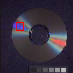
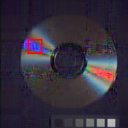
To visually compare the recovered results, we present visual illustrations of the recovered results obtained by different methods in Figs. 3-6. Aiming at a better visual comparison, we mark one local area and enlarge it under each image. From Figs. 3-6, we can observe that all the compared methods can somewhat recover the multi-dimensional data. The results of TNN and TRLRF contain some spatial blurring effects on MSIs (e.g., Cd and Beads). Although the FTNN and FCTN have better recovery effects than TNN and TRLRF visually, there are still some unsatisfactory performance in local details. The results of HLRTF have more spatial edges or textures compared to FTNN and FCTN, but small blurring effects still can be found. On the contrary, the proposed DTR performs better on the preservation of global structure and local details compared with the comparative methods.
Overall, the proposed DTR achieves superior performance on multi-dimensional data, including HSIs, MSIs, and videos. The superior performace of DTR can be attributed to the powerful representation ability of deep latent generative module and deep transform module. These two indispensable components allow DTR to more faithfully capture the rich textures and details in multi-dimensional data, which is particularly beneficial for multi-dimensional data recovery tasks.
VI Discussions
Two indispensable components (i.e., the deep latent generative module and the deep transform module) in the proposed DTR framework complement to each other and work together to make up a unified framework. In this section, we discuss the roles of each component in the DTR framework.
VI-A The Contribution of Deep Latent Generative Module
VI-A1 Deep Latent Generator vs Shallow Matrix Factorization
To verify the characterization ability of deep latent generator, we compare the recovered results by the shallow characterization-based method (i.e., based on NMF) and deep characterization-based methods (i.e., based on deep latent generators). Table III shows the quantitative comparison of the proposed DTR variants with different latent tensor characterizations for HSI Pavia. We can observe that the recovered results of shallow characterization-based method are generally inferior to that of deep characterization-based methods, and the number of network parameters is much larger. It is rational to say that the deep latent generator is more effective and efficient than shallow matrix factorization.
| Sampling rate | 0.1 | 0.2 | 0.3 | Params | ||||
|---|---|---|---|---|---|---|---|---|
| PSNR | SSIM | PSNR | SSIM | PSNR | SSIM | (M) | ||
| Shallow | NMF | 41.71 | 0.9845 | 46.75 | 0.9948 | 49.09 | 0.9968 | 2.102 |
| V-Net | 43.09 | 0.9880 | 44.79 | 0.9918 | 45.95 | 0.9933 | 0.165 | |
| Deep | DenseNet | 43.20 | 0.9881 | 48.80 | 0.9963 | 49.71 | 0.9971 | 0.659 |
| U-Net | 45.87 | 0.9942 | 48.85 | 0.9966 | 50.22 | 0.9974 | 0.565 | |
| U-Net-3D | 46.32 | 0.9945 | 49.33 | 0.9969 | 50.40 | 0.9975 | 1.388 | |
VI-A2 The Influence of Different Networks
Deep latent generative module plays a paramount role in the proposed DTR. We compare the recovered results by the proposed DTR with three classic networks, i.e., V-Net [40], DenseNet [41], and U-Net [42]. Table III shows the quantitative comparison of different DTR variants for HSI Pavia, where “U-Net-3D” denotes the U-Net using 3D filters. We can observe that U-Net achieves better results compared to V-Net and DenseNet, which indicates that the U-Net may be a good choice for generating the latent tensor. In addition, while U-Net-3D achieves better recovery results compared to U-Net, it comes with nearly double number of parameters as U-Net. Considering the trade-off between efficiency and performance, we set the as U-Net in our experiments.
VI-A3 The Influence of the Layer Number of
The layer number of deep latent generative module is a crucial parameter that determines the characterization ability of . Table IV presents the quantitative comparison of the proposed DTR with different layer number of for HSI Pavia. As shown in Table IV, we can observe that increasing enhances the performance when is small. However, when becomes larger, the results are not as desirable as expected. This is because a deeper network is more likely to suffer from the vanishing gradient. In our experiments, we set the layer number of to 2 to strike a balance between performance and the risk of vanishing gradient.
| Sampling rate | 0.1 | 0.2 | 0.3 | Params | ||||
| PSNR | SSIM | PSNR | SSIM | PSNR | SSIM | (M) | ||
| = 1 | 37.13 | 0.9555 | 39.27 | 0.9708 | 39.78 | 0.9743 | 0.095 | |
| = 2 | 45.87 | 0.9942 | 49.32 | 0.9968 | 50.22 | 0.9974 | 0.565 | |
| = 3 | 46.19 | 0.9942 | 47.86 | 0.9958 | 49.58 | 0.9970 | 2.412 | |
| = 4 | 45.34 | 0.9935 | 48.28 | 0.9963 | 49.08 | 0.9968 | 9.821 | |
| = 5 | 45.28 | 0.9933 | 48.39 | 0.9962 | 49.04 | 0.9968 | 103.423 | |
| = 1 | 45.10 | 0.9929 | 48.97 | 0.9967 | 49.79 | 0.9973 | 0.559 | |
| = 2 | 45.87 | 0.9942 | 49.32 | 0.9968 | 50.22 | 0.9974 | 0.565 | |
| = 3 | 45.49 | 0.9940 | 48.73 | 0.9965 | 49.81 | 0.9973 | 0.572 | |
| = 4 | 45.75 | 0.9939 | 48.66 | 0.9965 | 50.09 | 0.9973 | 0.578 | |
| = 5 | 45.46 | 0.9939 | 48.55 | 0.9965 | 49.54 | 0.9972 | 0.584 | |
| DTR Without | 44.36 | 0.9923 | 48.24 | 0.9961 | 49.74 | 0.9971 | 0.552 | |
VI-A4 The Influence of Value
To analyze the influence of value on recovery effects of the proposed DTR, we conduct quantitative comparison of the proposed DTR with different value for HSI Pavia in Table V. As shown in Table V, we can observe that a moderate can obtain a satisfactory recovery effects. To balance the performance of the proposed DTR and the computational complexity, we set in all our experiments.
| Sampling rate | 0.1 | 0.2 | 0.3 | Params | |||
|---|---|---|---|---|---|---|---|
| PSNR | SSIM | PSNR | SSIM | PSNR | SSIM | (M) | |
| = | 44.95 | 0.9931 | 47.19 | 0.9956 | 49.02 | 0.9967 | 0.531 |
| = | 44.99 | 0.9933 | 48.60 | 0.9964 | 50.27 | 0.9974 | 0.542 |
| = | 45.87 | 0.9942 | 49.32 | 0.9968 | 50.22 | 0.9974 | 0.565 |
| = | 45.72 | 0.9941 | 48.97 | 0.9968 | 50.40 | 0.9975 | 0.611 |
VI-B The Contribution of Deep Transform Module
The deep transform module is another indispensable component in the proposed DTR. Table IV presents the quantitative comparison of the proposed DTR with different the layer number of for HSI Pavia. It can be observed that using the deep transform module can achieve better recovered results, which reflects the effectiveness of deep transform module. Particularly, when = 1, degenerates into a linear transform. We can observe that nonlinear transform (i.e., ) can achieve better recovered results, which indicates that nonlinear transform can better capture the frontal slice relationships of multi-dimensional data. Similar to the deep latent generative module, we can observe that increasing enhances the performance when is small. However, when becomes larger, the performance tends to drop. Thus, in our experiments, we set the layer number of to 2.
VII Conclusion
In this paper, we proposed a unified deep tensor representation (termed as DTR) framework by synergistically combining the deep latent generative module and the deep transform module. The new DTR framework not only allows us to better understand the classic shallow representations, but also leads us to explore new representation. Extensive experiments demonstrate that the proposed DTR can achieve satisfactory performance on multi-dimensional data recovery problems.
References
- [1] C. Huang, M. K. Ng, T. Wu, and T. Zeng, “Quaternion-based dictionary learning and saturation-value total variation regularization for color image restoration,” IEEE Transactions on Multimedia, vol. 24, pp. 3769–3781, 2022.
- [2] Y. Liu, Z. Long, and C. Zhu, “Image completion using low tensor tree rank and total variation minimization,” IEEE Transactions on Multimedia, vol. 21, no. 2, pp. 338–350, 2019.
- [3] F. Fang, T. Wang, Y. Wang, T. Zeng, and G. Zhang, “Variational single image dehazing for enhanced visualization,” IEEE Transactions on Multimedia, vol. 22, no. 10, pp. 2537–2550, 2020.
- [4] A. Anandkumar, R. Ge, D. Hsu, S. M. Kakade, and M. Telgarsky, “Tensor decompositions for learning latent variable models,” Journal of Machine Learning Research, vol. 15, pp. 2773–2832, 2014.
- [5] S. Gandy, B. Recht, and I. Yamada, “Tensor completion and low-n-rank tensor recovery via convex optimization,” Inverse problems, vol. 27, no. 2, p. 025010, 2011.
- [6] Z. Fabian, R. Heckel, and M. Soltanolkotabi, “Data augmentation for deep learning based accelerated MRI reconstruction with limited data,” in International Conference on Machine Learning, 2021, pp. 3057–3067.
- [7] X. Li, Y. Ye, and X. Xu, “Low-rank tensor completion with total variation for visual data inpainting,” in Proceedings of the AAAI Conference on Artificial Intelligence, vol. 31, 2017, pp. 2210–2216.
- [8] J. Tian, Z. Han, W. Ren, X. Chen, and Y. Tang, “Snowflake removal for videos via global and local low-rank decomposition,” IEEE Transactions on Multimedia, vol. 20, no. 10, pp. 2659–2669, 2018.
- [9] J. You, X. Li, M. Low, D. Lobell, and S. Ermon, “Deep gaussian process for crop yield prediction based on remote sensing data,” in Proceedings of the AAAI Conference on Artificial Intelligence, vol. 31, 2017, pp. 4559–4566.
- [10] H. Li, R. Feng, L. Wang, Y. Zhong, and L. Zhang, “Superpixel-based reweighted low-rank and total variation sparse unmixing for hyperspectral remote sensing imagery,” IEEE Transactions on Geoscience and Remote Sensing, vol. 59, no. 1, pp. 629–647, 2021.
- [11] H. Zeng, J. Xue, H. Q. Luong, and W. Philips, “Multimodal core tensor factorization and its applications to low-rank tensor completion,” IEEE Transactions on Multimedia, pp. 1–15, 2022.
- [12] M. Lv, W. Li, T. Chen, J. Zhou, and R. Tao, “Discriminant tensor-based manifold embedding for medical hyperspectral imagery,” IEEE Journal of Biomedical and Health Informatics, vol. 25, no. 9, pp. 3517–3528, 2021.
- [13] H. Chen and J. Li, “Neural tensor model for learning multi-aspect factors in recommender systems,” in International Joint Conference on Artificial Intelligence, 2020, pp. 2449–2455.
- [14] Z. Chen, Z. Xu, and D. Wang, “Deep transfer tensor decomposition with orthogonal constraint for recommender systems,” in Proceedings of the AAAI Conference on Artificial Intelligence, vol. 35, 2021, pp. 4010–4018.
- [15] Z. Chen, J. Yao, G. Xiao, and S. Wang, “Efficient and differentiable low-rank matrix completion with back propagation,” IEEE Transactions on Multimedia, vol. 25, pp. 228–242, 2023.
- [16] Z. Zhang, G. Ely, S. Aeron, N. Hao, and M. Kilmer, “Novel methods for multilinear data completion and de-noising based on Tensor-SVD,” in Proceedings of the IEEE Conference on Computer Vision and Pattern Recognition, 2014, pp. 3842–3849.
- [17] Y.-S. Luo, X.-L. Zhao, D.-Y. Meng, and T.-X. Jiang, “HLRTF: Hierarchical low-rank tensor factorization for inverse problems in multi-dimensional imaging,” in Proceedings of the IEEE Conference on Computer Vision and Pattern Recognition, 2022, pp. 19 281–19 290.
- [18] X.-L. Zhao, W.-H. Xu, T.-X. Jiang, Y. Wang, and M. K. Ng, “Deep plug-and-play prior for low-rank tensor completion,” Neurocomputing, vol. 400, pp. 137–149, 2020.
- [19] T.-X. Jiang, T.-Z. Huang, X.-L. Zhao, and L.-J. Deng, “Multi-dimensional imaging data recovery via minimizing the partial sum of tubal nuclear norm,” Journal of Computational and Applied Mathematics, vol. 372, p. 112680, 2020.
- [20] T.-X. Jiang, M. K. Ng, X.-L. Zhao, and T.-Z. Huang, “Framelet representation of tensor nuclear norm for third-order tensor completion,” IEEE Transactions on Image Processing, vol. 29, pp. 7233–7244, 2020.
- [21] C. Lu, X. Peng, and Y. Wei, “Low-rank tensor completion with a new tensor nuclear norm induced by invertible linear transforms,” in Proceedings of the IEEE Conference on Computer Vision and Pattern Recognition, 2019, pp. 5989–5997.
- [22] B. Madathil and S. N. George, “DCT based weighted adaptive multi-linear data completion and denoising,” Neurocomputing, vol. 318, pp. 120–136, 2018.
- [23] M. E. Kilmer and C. D. Martin, “Factorization strategies for third-order tensors,” Linear Algebra and Its Applications, vol. 435, no. 3, pp. 641–658, 2011.
- [24] P. Zhou, C. Lu, Z. Lin, and C. Zhang, “Tensor factorization for low-rank tensor completion,” IEEE Transactions on Image Processing, vol. 27, no. 3, pp. 1152–1163, 2018.
- [25] F. Wu, Y. Li, C. Li, and Y. Wu, “A fast tensor completion method based on tensor QR decomposition and tensor nuclear norm minimization,” IEEE Transactions on Computational Imaging, vol. 7, pp. 1267–1277, 2021.
- [26] C. Lu, J. Feng, Y. Chen, W. Liu, Z. Lin, and S. Yan, “Tensor robust principal component analysis with a new tensor nuclear norm,” IEEE Transactions on Pattern Analysis and Machine Intelligence, vol. 42, no. 4, pp. 925–938, 2020.
- [27] M. K. Ng, X. Zhang, and X.-L. Zhao, “Patched-tube unitary transform for robust tensor completion,” Pattern Recognition, vol. 100, p. 107181, 2020.
- [28] G. Song, M. K. Ng, and X. Zhang, “Robust tensor completion using transformed tensor singular value decomposition,” Numerical Linear Algebra with Applications, vol. 27, no. 3, p. e2299, 2020.
- [29] T.-X. Jiang, X.-L. Zhao, H. Zhang, and M. K. Ng, “Dictionary learning with low-rank coding coefficients for tensor completion,” IEEE Transactions on Neural Networks and Learning Systems, vol. 34, no. 2, pp. 932–946, 2023.
- [30] H. Kong, C. Lu, and Z. Lin, “Tensor Q-rank: new data dependent definition of tensor rank,” Machine Learning, vol. 110, no. 7, pp. 1867–1900, 2021.
- [31] Y. Zheng and A.-B. Xu, “Tensor completion via tensor QR decomposition and -norm minimization,” Signal Processing, vol. 189, p. 108240, 2021.
- [32] M. E. Kilmer, K. Braman, N. Hao, and R. C. Hoover, “Third-order tensors as operators on matrices: A theoretical and computational framework with applications in imaging,” SIAM Journal on Matrix Analysis and Applications, vol. 34, no. 1, pp. 148–172, 2013.
- [33] T. G. Kolda and B. W. Bader, “Tensor decompositions and applications,” SIAM Review, vol. 51, no. 3, pp. 455–500, 2009.
- [34] Y.-S. Luo, X.-L. Zhao, T.-X. Jiang, Y. Chang, M. K. Ng, and C. Li, “Self-supervised nonlinear transform-based tensor nuclear norm for multi-dimensional image recovery,” IEEE Transactions on Image Processing, vol. 31, pp. 3793–3808, 2022.
- [35] Z. Li, T. Sun, H. Wang, and B. Wang, “Adaptive and implicit regularization for matrix completion,” SIAM Journal on Imaging Sciences, vol. 15, no. 4, pp. 2000–2022, 2022.
- [36] J. Fan and J. Cheng, “Matrix completion by deep matrix factorization,” Neural Networks, vol. 98, pp. 34–41, 2018.
- [37] D. P. Kingma and J. Ba, “Adam: A method for stochastic optimization,” in International Conference on Learning Representations, 2015.
- [38] L. Yuan, C. Li, D. Mandic, J. Cao, and Q. Zhao, “Tensor ring decomposition with rank minimization on latent space: An efficient approach for tensor completion,” in Proceedings of the AAAI Conference on Artificial Intelligence, vol. 33, 2019, pp. 9151–9158.
- [39] Y.-B. Zheng, T.-Z. Huang, X.-L. Zhao, Q. Zhao, and T.-X. Jiang, “Fully-connected tensor network decomposition and its application to higher-order tensor completion,” in Proceedings of the AAAI Conference on Artificial Intelligence, vol. 35, 2021, pp. 11 071–11 078.
- [40] F. Milletari, N. Navab, and S.-A. Ahmadi, “V-Net: Fully convolutional neural networks for volumetric medical image segmentation,” in 2016 Fourth International Conference on 3D Vision, 2016, pp. 565–571.
- [41] G. Huang, Z. Liu, L. van der Maaten, and K. Q. Weinberger, “Densely connected convolutional networks,” in Proceedings of the IEEE Conference on Computer Vision and Pattern Recognition, 2017, pp. 2261–2269.
- [42] O. Ronneberger, P. Fischer, and T. Brox, “U-Net: Convolutional networks for biomedical image segmentation,” in Medical Image Computing and Computer-Assisted Intervention, 2015, pp. 234–241.