Drone-Delivery Network for Opioid Overdose - Nonlinear Integer Queueing-Optimization Models and Methods
Abstract
We propose a new stochastic emergency network design model that uses a fleet of drones to quickly deliver naloxone in response to opioid overdoses. The network is represented as a collection of queueing systems in which the capacity of each system is a decision variable and the service time is modelled as a decision-dependent random variable. The model is an optimization-based queueing problem which locates fixed (drone bases) and mobile (drones) servers and determines the drone dispatching decisions, and takes the form of a nonlinear integer problem intractable in its original form. We develop an efficient reformulation and algorithmic framework. Our approach reformulates the multiple nonlinearities (fractional, polynomial, exponential, factorial terms) to give a mixed-integer linear programming (MILP) formulation. We demonstrate its generalizablity and show that the problem of minimizing the average response time of a collection of queueing systems with unknown capacity is always MILP-representable. We design an outer approximation branch-and-cut algorithmic framework which is computationally efficient and scales well. The analysis based on real-life data reveals that drones can in Virginia Beach: 1) decrease the response time by 82%, 2) increase the survival chance by more than 273%, 3) save up to 33 additional lives per year, and 4) provide annually up to 279 additional quality-adjusted life years.
Key words: opioid overdose, drone delivery, optimization-based queueing model, survival chance, mixed-integer nonlinear programming, stochastic network design
1 Introduction
From 1999 to 2019, almost 500,000 people died from overdose in the USA [21] which is the leading cause of death for 25- to 64-year old US citizens. Opioid overdose is a life-threatening condition that, if not treated within minutes, can lead to severe neurological damage and death [18]. The chance of survival of an opiate overdose victim decreases by 10% with each minute passing before resuscitation is attempted [64]. Although emergency medical services (EMS) are located to optimize access to the population, the median arrival time of US EMS is between 7 and 8 minutes and can go beyond 14 minutes in rural, geographically- challenged, or high-traffic urban areas [43]. In that respect, [36] [36] report that lessening the response time by one minute traditionally requires adding ambulances, each costing around $200,000, whereas a $10,000 drone can decrease the response time by two minutes. Consequently, medical drones are viewed as a promising way to reduce response times and to enhance EMS performance [66]. This motivates us to design a drone-based network to provide timely medical treatment and to study its potential to increase the chance of survival of overdose victims.
1.1 Background
The opioid overdose epidemic is ramping up as the number of incidents has quadrupled in the last 15 years. In the midst of this crisis, there are about 130 opioid overdose deaths each day [64]. The first wave of overdoses began in 1990s and was associated to prescription opioids. The 2010 second wave was due to heroin while the third one in 2013 was caused by synthetic opioids, in particular the illicitly manufactured fentanyl [19]. The ongoing COVID-19 pandemic has further exacerbated the opioid health crisis. According to the Centers for Disease Control and Prevention (CDC) [20], over 81,000 drug overdose deaths occurred in the USA between May 2019 and May 2020. Synthetic opioids are the primary driver behind the surge in overdose deaths. The death counts related to the synthetic opioid increased by 38.4% from the 12-month period ending in June 2019 to the 12-month period ending in May 2020. In addition to the substantial human toll, opioid overdose poses a great burden on the economy. The Society of Actuaries [74] estimates that the economic cost of opioid misuse amounts to at least $631 billions from 2015 to 2019 in the USA and includes the cost for healthcare services, premature mortality, criminal justice activity, and related educational and assistance program. The White House Council of Economic Advisers (CEA) estimates the 2015 total cost of opioid overdoses to $504 billion with $431.7 billion due to mortality costs and $72.3 billion due to health, productivity, and criminal justice costs [16].
Many overdose-related deaths are preventable if naloxone, an overdose-reversal medication, can be delivered within minutes following the breath cessation of the overdose victim [18]. Naloxone can be safely administered by a layperson witnessing an overdose incident [77] and its increased utilization has contributed to reducing the mortality rate of opioid overdoses as stressed in [50]. As opioids can slow down or even entirely stop breathing, permanent brain damage can occur within only four minutes of oxygen deprivation. This underscores the need of administering naloxone timely to prevent brain damages or death and explains why naloxone access is of the US Department of Health and Human Services’ three priority areas to combat the opioid crisis [44]. In order to mitigate the opioid crisis, [64] [64] advocate the development of a system that allows 911 dispatchers, trained as drone pilots, to swiftly deliver naloxone with drones to bystanders and to guide them to administer naloxone.
Drones, also known as unmanned aerial vehicles (UAVs), are an emerging technology that can accomplish time-sensitive medical delivery tasks by fastening the time-to-scene response, particularly in the areas lacking established transportation network. A test in Detroit showed that the DJI ’Inspire 2’ drones turned out to be systematically faster than ambulances – the traditional first responders – in delivering a naloxone nasal spray toolkit [75]. In order to make drone deliveries of naloxone a reality and to leverage their full capability, drones need to be strategically deployed and assigned in a timely manner to the randomly arriving overdose-triggered requests (OTRs) to account for the spatial and temporal uncertainty of opioid overdose incidents. The design of drone networks that sets up drone bases, pre-positions drones, and determines their assignment to overdose emergencies remains an open problem in the literature. In that regard, [18] [18] stress the need to develop drone network optimization models for opioid overdoses so that dispatchers “understand when and where to dispatch drones”.
1.2 Structure and Contributions
The contributions of this study are fourfold spanning across modeling, reformulation, algorithmic development, and emergency medical service practice.
Modeling: We develop a novel network design queueing-optimization model to help EMS operators respond quickly and efficiently to an opioid overdose via the drone-based delivery of naloxone. The proposed model is a stochastic service system design model with congestion [7] and represents the drone network as a collection of queueing systems. The model determines the location of drone bases (DB) and drones as well as the dispatching of drones to overdose incidents. The model has two distinct and novel features. First, while some studies consider queueing systems in which is a decision variable, our optimization model is the first one – to our knowledge – to consider queueing systems (which generalize the system) in which the number of mobile servers (system capacity) is a decision variable. The possibility to adjust the capacity of the queueing system is a critical feature. A recent study [15] argues that “an integrated location-queueing model that simultaneously optimizes the location and number of drone resources can reduce overall resource needs by more than 50% without degrading performance”. Second, while the travel time between facilities and demand locations is for mobile servers an integral part of the service time, which hence depends on location and assignment decisions, the extant literature assumes that the average service time and the service rate are constants known a priori. Contrasting with this, our model represents the service time, and thus the queueing delay and response time, as functions of the location and assignment decisions. This modeling approach allows us to capture the decision-dependent uncertain nature of the service time whose expected value is calculated endogenously, and can be applied (and even be more beneficial) for other mobile server networks (e.g., ambulances, helicopters) in which the travel time can be a larger portion of the service time. We are not aware of any such model in the literature.
Reformulation: The base formulation of the proposed drone network design model is a nonlinear integer problem which includes fractional, polynomial, exponential, and factorial terms. We derive in Theorem 3 a lifted mixed-integer linear programming (MILP) reformulation. Theorem 4 shows that the reformulation method is highly generalizable and that optimization models minimizing the average network response time of a series of interdependent queueing systems with unknown number of servers are always MILP-representable.
Algorithm: We design two outer approximation methods to solve the lifted MILP reformulation. The first one is an outer approximation algorithm based on the concept of lazy constraints to attenuate the challenges due to the large dimension of the constraint space. The second algorithm is an outer approximation branch-and-cut algorithm that involves the dynamic incorporation of valid inequalities and optimality cuts. The computational study shows that the second algorithm based on the reduced-size MILP reformulation is the most efficient and scalable, and solves to optimality all problem instances in one hour while Gurobi only solves 10% of those. We show that the reduced response times are not only due to drones but also to our modeling approach which significantly increases the chance of survival as compared to using greedy heuristics and a benchmark model. In short, this study fills in the research gap underlined by [18] who argue that further research is needed “to develop a decision support system to aid the 911 dispatchers to efficiently assign the drones in a time-sensitive environment” such as opioid overdoses and that “such decision support requires advances in resource allocation and optimization algorithms that consider under-resourced environment”.
Data-driven EMS insights: Using real-life overdose data, we demonstrate the extent to which the drone network contributes in reducing the response time, in increasing the survival chance of overdose victims, and thereby in saving lives. The cross-validation, the comparison with another model and two greedy heuristic methods, and the simulations analyses underline the applicability and robustness of the network and its performance. Additional tests attest the low cost of a drone network and its flexibility to adjust to the spatio-temporal uncertainty of overdose incidents. The quality-adjusted life year (QALY) underscores the largely increased quality of life and the low incremental QALY cost.
The remainder of this paper is organized as follows. The literature review of the various fields intersecting with this study is in Section 2. Section 3 derives the closed-form formulas for the queueing metrics used to assess the performance of the drone response network, presents the base formulation of the model, and analyzes its complexity. Section 4 is devoted to the reformulation method while Section 5 describes the algorithms. Section 6 describes the numerical study based on overdose real-life data from Virginia Beach, presents the computational efficiency of the method, and analyzes the healthcare benefits obtained with our model. Section 7 provides concluding remarks. We refer the reader to Appendix A for a list of the acronyms used in this paper and to Appendix B for a list of the mathematical notations.
2 Literature Review and Gaps
This study propose contributions spanning across three fields – drone-based response to medical emergencies, network design queueing models with mobile servers, and fractional 0-1 programming - which we review below.
2.1 Drone-based Response to Medical Emergencies
EMSs struggle to provide a timely response to medical emergencies leading to patients passing away due to the delayed arrival of ground ambulances. Medical drones are viewed as an efficient solution to assist EMS professionals, including for overdoses. They can quickly deliver medicine to patients and take on-sight imagery to support EMS personnel and operations before the arrival of ambulances [66]. We review next the literature on the use of drones for medical emergencies. We focus on overdoses, the topic of this study, and cardiac arrests to which most drone-related studies have been devoted in the medical sphere [59]. We refer the reader to [70] for a recent review on the use of drones in health care.
[79] [79] propose a drone-delivery optimization model for overdoses solved with a genetic algorithm and tested on suspected opioid overdose data from Durham County, NC. The model reduces the response time to 4 minutes 38 seconds by using four drone bases and provides a 64.2% coverage of the county. [36] [36] propose a Markov decision process model that selects which drone should be dispatched to an overdose incident and then relocates the drone. Confronted with the curse of dimensionality, the authors develop a state aggregation heuristic to derive a lookup table policy. A simulation based on EMS data from Indiana reveals that the state aggregation approach outperforms the myopic policy used in practice, in particular when the overall request intensity gets higher, but also highlights the difficulty to estimate the value function. [64] [64] report that all participants in a pilot feasibility study based on 30 simulated opioid overdoses were able to administer the intranasal naloxone medication to the manikin within about two minutes after the 911 call and that 97% of them felt confident that they could do it successfully in a real event.
We now review the drone literature for out-of-hospital cardiac arrests (OHCA). Scott and Scott [72] propose two set covering formulations based on a tandem air-ground response to OHCAs. The models set up the location of the depots (where ground vehicles are stationed) and drone bases without taking into account congestion. Medical supplies are delivered with a ground-based vehicle from a depot to a drone location and the last-mile delivery to the OHCA location is carried out with a drone. Pulver et al. [68] determine where to set up drone bases in order to maximize the number of OHCA requests responded to within one minute. This coverage-type facility location model does not concern with the possible congestion of the network and assumes that the demand and the drone response times are deterministic. Pulver and Wei [67] propose a multi-objective set covering model with backup coverage. Decisions pertaining to the positioning of drones and their assignment to OHCAs are taken to maximize the backup and primary coverage of the network. Boutilier et al. [13] present a two-step approach to design a drone network delivering automated external defibrillators. In the first step, a set covering model is solved approximately to determine the number of drone bases needed to reduce the median response time. In the second step, an queueing model determines heuristically the number of drones at each base. The opened stations are fixed (determined in the first stage), and the arrival rate and expected service time are defined as fixed parameters determined ex-ante. Boutilier and Chan [15] propose two coverage-type models that minimize the number of drones needed to satisfy a response time target (i.e., decrease in expected value or conditional value-at-risk of response time). The models do not reward, nor incentivize faster response times. For example, if the target is to decrease the response time by, say, 20 seconds, the models consider a 20-second and an 80-second reduction in the response time as equally satisfactory. The queueing models underlying the formulations assume that the service and response times are independent from the utilization of drones. Mackle et al. [51] present a genetic algorithm to calculate the number of drone bases needed to satisfy a response time threshold. Bogle et al. [10] use a coverage-type facility location model to determine the number and location of drone stations so that a specified number of at-risk OHCA victims are reachable within a certain time. Cheskes et al. [23] use simulation to examine the feasibility and benefits of using drones for OHCAs in rural and remote areas.
The above models assume that the average service time is fixed and independent from the drone assignment decisions. Additionally, they are all covering models in which the objective function is to minimize the total costs or the number of drones (bases) but does not reward a quicker response. Our model contributes to fill in the gaps in the literature. Our strategic network model (i) is a survival network design model as it minimizes the response time which is the primary driver to increase the survival chance of overdosed patients; and (ii) represents the service time as a distribution-free decision-dependent random variable with service rate defined endogenously as a function of the drone dispatching policy.
We explain next how our model differs significantly from the OHCA models proposed in [15] which have, as our model, a queueing underlying structure. First, the objective in [15] to minimize the number of DBs is typical in coverage-type facility location models which, as noted in the literature, are unable to differentiate the impact of varying response times [32], or to reward shorter ones and whose suitability for time-critical medical events has been extensively questioned (see, e.g., [32, 42, 60]). In contrast, our model explicitly rewards quick response time and is hence conducive to maximizing the number of opioid overdose incident survivors. As the overdosed patients’ chance of survival rapidly deteriorates with the time-to-treatment, it is critical to use an objective function which provides a reward diminishing with the time needed to respond. The maximization of the QALY is an alternative objective function that could fulfill the true needs of a medical emergency response network. Second, the underlying queueing models in [15] assume that the service times are exponentially distributed with fixed rates (fixed average service time regardless of drones’ placement) and that the response time between any pair of drone bases and OHCAs incidents is fixed ex-ante and independent from drone utilization and network congestion. Such assumptions do not allow for an accurate representation of the queueing system as explained in a 2023 study [78]. The authors [78] demonstrate that it is critical to track the actual utilization of facilities and servers so that the known impact of utilization can be accurately reflected on the congestion level, waiting time, and response time. Along the same line, it was previously shown [60] that assuming that facilities’ workloads are known a priori and that each facility can provide the same service level irrelevant of their actual utilization significantly hurts the network’s efficiency and reliability. We do not resort to such simplifying assumptions and instead model the opioid overdose arrival rate, the service rate, and the average response times as unknowns dependent on the utilization of the resources and the assignment policy, and define them as decision variables whose values are determined endogenously by the model.
2.2 Queueing-optimization Models for Stochastic Network Design
Queueing models can be categorized into two types: descriptive queueing models which conduct an after-the-fact analysis to analyze how a predefined system configuration has performed while optimization-based (prescriptive) queueing models deal with congestion and are used for decision-making purposes (e.g., number of servers, location) [53]. We propose a new optimization-based queueing model that belongs to the class of stochastic network design queueing models with congestion [7]. This model class can be further decomposed into two sub-categories depending on whether the servers are fixed (immobile) requesting the customers to travel to the facility, or mobile and travel to the demand location. Since we consider the delivery of naloxone with drones, our literature review is focused on mobile servers, which is much less extensive than the one for immobile servers (see, e.g., [37]).
The first queueing optimization model with mobile server [9] determines the optimal location of a single facility in order to either maximize the service coverage or to minimize the response cost. Modelling the network as an system, the authors consider that, if the server is busy when the demand arrives, the demand can be either rejected (demand is lost and covered by backup servers at a cost) or enter a queue managed under the first-come-first-serve discipline. Building on this study, Chiu and Larson [24] consider a single facility operating as an loss queueing system and show that, under a mild assumption, the optimal location reduces to a Hakimi median, which minimizes the average travel time to a client. Batta and Berman [5] study an system and develop an an approximation-based approach to minimize the average response time. While the above studies consider a single facility, the queueing probabilistic location set-covering model proposed in [53] considers several facilities, each operating as an queueing system. The authors determine the minimum number of facilities needed so that the probability of at least one server being available is greater than or equal to a certain threshold. Later, operating under the auspices of an system, Marianov and Revelle [52] study the probabilistic version of the maximal covering problem to site a limited number of emergency vehicles with the goal of maximizing availability when a call arrives. Considering an system, [1] [1] determine the number of servers needed to minimize the setup costs to open facilities and operate servers, the travel costs, and the queueing delay costs. In the EMS context, [13] [13] propose a decoupled approach to design a drone network for OHCAs. Each DB operates as an system in which the expected service time and the arrival rate are fixed parameters. The coverage-type queueing models in [15] minimize the number of drones needed to satisfy a response time target. They assume that the service rates and response times are fixed and independent from the utilization of the drones, their positioning at DBs, and the congestion in the network. The queueing models in [15] extend the one in [54] for fixed servers and in which the objective is to minimize the number of facilities so that the waiting time or queue size does not exceed a set threshold. An ongoing study [46] considers an queueing system for responding to cardiac arrests and proposes new optimality-based bound tightening techniques. In contrast to the above health care studies, this work considers that the service times, the delays, the response times, and the arrival process of (overdose) requests assigned to drones are random variables whose parameters (mean) are endogenized. In particular, the response times and the service rates are decision variables whose values are determined by the model and depend on assignments.
2.3 Fractional Nonlinear 0-1 Programming
As it will be shown in Section 3.3, the optimization problem studied is a nonlinear fractional integer problem in which the objective function is a ratio of two nonlinear functions each depending on integer variables. The class of problems closest to ours is that of fractional linear 0/1 (binary) problems for which significant improvements have been made over the last years [11, 58]. Such problems arise in multiple applications, such as chemical engineering, clinical trials, facility location [48], product assortment [17], and revenue management (see [12] for a review). We also note a few fractional mixed-integer queueing-optimization problems (see, e.g., [37, 31, 39]. Such problems pose serious computational challenges due to the pseudo-convexity and the combinatorial nature of the fractional objective. They minimize a single or a sum of ratios in which the denominator and numerator are linear functions of binary variables. When more than one ratio term is in the objective function, the problem, even unconstrained, is NP-hard [65].
One approach to tackle fractional linear 0-1 programs is to move the fractional terms to the constraint set and to then derive MILP reformulations, which requires the introduction of continuous auxiliary variables and big-M constraints (see, e.g., [47]). However, MILP solvers have difficulties – in particular when the number of ratio terms increases – due to the significant lifting of the decision and constraint spaces and the looseness of the continuous relaxation induced by the big-M constraints. Within this family, the MILP reformulation proposed in [11] and based on the binary expansion of the integer-valued expressions in the ratio terms contains many less bilinear terms and hence less linearization variables and constraints. This formulation scales much better but can generate weak continuous relaxations, which hurts the convergence of the branch-and-bound algorithm. Mixed-integer second-order cone reformulations have also been proposed (e.g., [73]). They are based on the submodularity concept and the derivation of extended polymatroid cuts [3] to obtain tighter continuous relaxations. However, it is reported [58] that state-of-the-art optimization solvers still struggle to solve moderate-size mixed-integer conic problems and that their performance degrades quickly as size increases. Building upon the links between MILP and mixed-integer conic reformulations, [58] [58] derive tight convex continuous relaxations while limiting the lifting of the decision and constraint spaces.
The above methods, while providing very valuable insights, can not be directly used to the problem tackled here as the latter differs from the fractional 0-1 problem along several dimensions. First, the denominator and the numerator of each ratio term are nonconvex functions and each involve binary as well as general integer decision variables. Second, the objective function is the sum of a very large number (i.e., several thousands) of ratio terms. Third, the integer variables are multiplied by fractional parameters which prohibits the use of the MILP method (see [11]). Fourth, the nonlinear terms are not simply bilinear. The numerator of each ratio term includes exponential terms and higher-degree polynomial terms while each denominator includes polynomial and factorial terms.
3 Drone Network Design Problem for Opioid Overdose Response
3.1 Problem Description and Notations
The problem studied in this paper is called the Drone Network Design Problem for Opioid Overdose Response (DNDP). Consider an EMS provider that seeks to design a drone network to deliver naloxone, i.e., an opioid antagonist, to an opioid overdose incident with the objective to minimize the response time and thereby to maximize the chance of survival of the overdosed patient. Given a set of candidate locations (e.g., fire, police, EMS stations), some of them are selected to be set up as DBs where the available medical drones can be deployed. The DNDP model is a bilocation-allocation problem that simultaneously determines the locations of the DBs, the capacity of those (i.e., number of drones at each DB), and the response policy determined by the assignment of drones to OTRs in order to minimize the response time. The response time is defined as the sum of the queueing delay time experienced if drones are busy when requested for service and the drone flight time from a DB to an OTR location. The network is capacitated to account for the severely limited availability of medical resources. Considering the opioid epidemic, Buckland et al. [18] stress that the amount of medical resources (drones, ambulances, paramedics) is “substantially smaller than the number of patients who require immediate care”.
The following notational set is used in the formulation of the model (see Appendix B). Let be the set of OTR locations and be the set of potential DB locations. Let be a vector of parameters representing the coordinates of DB in the earth-centered, earth-fixed coordinate system while is a vector of parameters representing the location of an OTR. The parameter is the euclidean distance between DB and OTR location . A number of drones with speed can be deployed at up to open DBs across the network. Due to battery and autonomy limitations, each drone has a limited coverage defined by its catchment area with radius . A drone can only service OTRs that are within its catchment radius [13], since the drone must have battery coverage to return to its base. Accordingly, we define the sets (resp., ) which include all the DBs (resp., OTR locations) that are within of OTR location (resp, DB ). The binary decision variable is 1 if a DB is set up at location , and is 0 otherwise. The binary variable takes value 1 if an OTR at is assigned to DB and value 0 otherwise. The general integer decision variable is the number of drones deployed at DB . By convention, we denote the upper and lower bound of any decision variable by and , respectively.
3.2 DNDP Model: Collection of Queueing Systems with Unknown Capacity
The stochastic nature of the occurrence of overdoses and the resulting uncertainty about the arrival rates of OTRs at DBs along with the uncertain service times can cause delays, requests being queued, and waiting times until a drone can be dispatched. In order to account for those, we model the network as a collection of queues in which each DB operates as an queueing system where the capacity of DB is a bounded general integer decision variable representing the number of drones to be deployed at DB . The occurrence of opioid overdoses at any location follows a Poisson distribution with arrival rate . The service time of drones is a random variable with general distribution and with known first and second moments. The arrival rate of OTRs at DB can be inferred to be a Poisson process since it is a linear combination of independent Poisson variables (i.e., weighted sum of assigned OTRs; see (5)). The arrival rate of OTRs at DBs is unknown ex-ante and is defined endogenously via the solution of the optimization problem. The same applies to the drone service time whose expected value is also endogenized. It follows that the arrival process, i.e., demand at DBs and the service times of drones are endogenous sources of uncertainty with decision-dependent parameter (expected value) uncertainty as coined in [40]. If a drone cannot be dispatched on the spot after reception of an OTR, the request is placed in a queue depleted in a first-come-first-served manner. After providing service, drones travel back to the DB to be cleaned, recharged, and prepared for the next trip [64].
We now derive steady-state closed-form expressions for the queueing metrics - response time, queueing delay, service time – needed to formulate the DNDP problem. We use the notations , , and to represent the random variables respectively denoting the total service time at DB , the response time for an overdose at location , and the queueing delay at DB .
Different from immobile servers, the travel time to and from the scene are included in the service time for mobile servers [8]. The service time for any OTR at serviced by DB [9] is , where is a constant that allows for different travel speeds, and and are independent and identically distributed (i.i.d) random variables representing the on-scene service time and the drone’s reset time (to be charged and prepared for the next demand), respectively. Let , with expected value . The expected value of the service time conditional to DB responding to an OTR at is:
| (1) |
The expected value of the total response time for is the sum of the expected service times for all the OTRs serviced (i.e., ) by the drones stationed at and depends on the dispatching variables
| (2) |
while the second moment of the total service time at DB is:
| (3) |
The service time follows a general unspecified distribution with known first and second moments and the opioid overdoses occur at each location according to a Poisson process with rate . Accordingly, each DB is modelled as an queueing system in which a variable and upper bounded number of drones can be stationed and whose expected queueing delay can be approximated [63, 69] as
| (4) |
which represents the expected waiting time until a drone is ready to be dispatched after reception of an OTR. The arrival rate of OTRs at DB is given by
| (5) |
which shows that the arrival rate is unknown ex-ante and depends on the assignment decisions , thereby highlighting the decision-dependent parameter uncertainty of the OTR arrivals at DBs.
The expected response time in steady-state for an OTR at location is:
| (6) |
Remark 1
Note that the response and service time differ in the healthcare context. For example, Bandara et al. [4] define the response time as “the time between the receipt of a call at the dispatch centre and the arrival of the first emergency response vehicle at the scene” while their definition of the service time is “the time required for an ambulance to return back to its original station after leaving the station to attend the call, which includes the transportation time of the patient to the hospital if needed”.
The metric used in our model is the average (over all overdoses) of the expected response time. We denote it by and refer to it as the average response time. The proof of Proposition 1 is in Appendix C.1.
Proposition 1
The functional form of the average response time is a fractional expression with nonlinear numerator and denominator:
| (7) |
3.3 DNDP Base Model: Fractional Nonlinear Integer Programming Problem
We present now the base formulation of the DNDP problem, which belongs to the family of nonlinear fractional integer problems, and analyze its complexity. Before presenting its formulation, we recall the most distinctive features of the proposed DNDP model. First, the minimization of the average response time is a survival objective function as it contributes to increasing the survival chance of the victims of opioid overdoses. The chance of survival is a monotone decreasing function of the response time (see, e.g., [4, 27]). By minimizing response time and rewarding quick care, our model effectively maximizes the chance of survival of overdosed victims, which is viewed in the health care literature as a survival optimization model. Second, the queueing-optimization model accounts for congestion and decision-dependent uncertainty as the service and arrival rates characterizing the Poisson arrival process and service times of OTRs at DBs are determined endogenously. Third, the capacity – number of drones positioned of each DB is not fixed ex-ante, but is a bounded decision variable.
The fractional nonlinear integer base formulation of problem DNDP is:
| (8a) | ||||
| (8b) | ||||
| (8c) | ||||
| (8d) | ||||
| (8e) | ||||
| (8f) | ||||
| (8g) | ||||
| (8h) | ||||
| (8i) | ||||
The objective function (8a) minimizes the average response time of the network, a key feature given the time-critical nature of opioid overdoses. Given that the queueing formulas used to represent the response time assume that the system is in steady-state, we introduce the nonlinear constraints (8b) to ensure the stability of the queueing system [57] as they prevent the arrival rate at any DB from being equal or larger than the service rate. Constraint (8c) makes sure that each OTR is serviced by exactly one drone while (8d) requires that an OTR can only be assigned to an open DB within the drone catchment area. Constraint (8e) limits from above the number of open DBs with the parameter . Constraint (8f) ensures that drones can only be placed at an opened DB and that an opened DB must have at least one drone. The parameter defines the maximum number of drones that can be stationed at any DB . As suggested in [61] and as implemented in [6, 67, 36] for medical drone networks, we set equal to two as drones are scarce resources and are typically spread to expand the coverage of the network. Additionally, our preliminary tests based on real-life data show that giving the possibility to place a third drone at a DB does not reduce the response times. Constraint (8g) ensures that all available drones are deployed. The binary and general integer nature of the decision variables are enforced by (8h) and (8i) with denoting the set of nonnegative integer numbers. Remark 2 summarizes several key features of the model.
Remark 2
Problem is a nonconvex optimization problem in which: (i) The objective function is neither convex, nor concave: the denominator and the numerator in each ratio term of the objective function are nonconvex functions; (ii) The ratio terms can involve division by 0 and be indeterminate; (iii) Any ratio term related to a location where no DB is set up in undefined; (iv) There is a mix of binary and bounded general integer variables; (v) The continuous relaxation of is a nonconvex problem.
4 Reformulation Framework
Remark 2 highlights that the base formulation is a fractional nonlinear integer problem which is extremely difficult to solve numerically even for small problem instances. We derive an equivalent and computationally tractable MILP reformulation. We first demonstrate in Theorem 3 that an MILP reformulation can be derived when the number of servers is two or less as relevant to the medical drone network problem (see [6, 61, 67]) before generalizing this result (Theorem 4) to any queueing system with variable number of servers at each . By convention, a superscripted index inside parentheses refers to the component of a vector (e.g., refers to the component of ).
4.1 MILP Reformulations
The derivation of an MILP reformulation is relatively complex and we split it into two main steps (see Proposition 2 and Theorem 3) to ease the exposition.
Proposition 2 proposes an equivalent reformulation taking the form of a fractional nonlinear binary problem R-BFP with nonconvex continuous relaxation. The proof is given in Appendix C.3.
Proposition 2
Let . The fractional nonlinear binary problem
| (9a) | ||||
| s.to | ||||
| (9b) | ||||
| (9c) | ||||
| (9d) | ||||
| (9e) | ||||
| (9f) | ||||
is equivalent to the fractional nonlinear integer problem .
The following comments are worth noting. A first difference with is that has only binary decision variables and does not include any general integer variables . The second difference and advantage of over is that the polynomial terms in the reformulation are of lower degree than those in . Third, in , there is no decision variable appearing in the upper limits of the summation operations, such as in . Fourth, there is no exponential term of form in . Fifth, the factorial terms in which, besides being nonlinear, can also be undefined if , are no longer present in in which they are replaced by the fixed parameters . The undefined issue is resolved since is at least equal to 1. The reformulation is valid for any value assigned to .
The constraints (8c)-(8e), (8h), and (9b)-(9f) representing the feasible area of problem R-BFP define collectively a linear binary feasible set which, to ease the notation, is thereafter referred to as:
| (10) |
We give in Appendix D the objective function of problem for a small network. Table 9 in Appendix E specifies the number of constraints and integer decision variables of each type in the base formulation and its reformulation .
Although simpler than , is still a challenging optimization problem as it involves polynomial and fractional terms and its continuous relaxation is nonconvex. We shall now demonstrate in Theorem 3 that the MILP problem is equivalent to and . The proof is split into two main steps that starts with the moving of the fractional terms from the objective function into the constraint set and continues with the linearization of the polynomial terms. To shorten the notations in the proof, we replace and by and , respectively. We first consider the medical drone network design problem DNDP in which (i.e., up to two servers per DB). Theorem 4 will later show that an MILP reformulation can be derived for any value of the parameter , or, in other words, for any queueing system in which the capacity of each system is unknown and variable.
We recall two well-known linearization methods for bilinear terms used in the proof of Theorem 3:
Theorem 3
Define the index sets . Let , , , and be continuous auxiliary variables used for the linearizization of bilinear terms. The MILP problem
| (13a) | |||||
| s.to | (13b) | ||||
| (13c) | |||||
| (13d) | |||||
| (13e) | |||||
| (13f) | |||||
| (13g) | |||||
| (13h) | |||||
is equivalent to the nonlinear integer problems and for =2.
The proof of Theorem 3 is given in Appendix C.4 and is decomposed into two main parts. The linearization part first demonstrates that the nonlinear problems B-IFP and R-BFP are MILP-representable. The compaction part shows that the number of linearization constraints and variables can be significantly reduced. This result is attained by first showing that , which is in turn used to prove that the two sets of linear inequalities (13h) and
| (14) |
are equivalent (i.e., the superscript in (14) is while it is in (13h)). In Section 6.4, we assess the computational benefits of the compaction approach by comparing the results with the compact MILP reformulation R-MILP and the larger-size MILP reformulation L-MILP
| (15) |
in which (14) replaces (13h) in R-MILP. Observe that the MILP reformulation L-MILP contains more decision variables and more linearization constraints than R-MILP.
In Appendix D, we give the objective formulation of problem for a small network.
4.2 Generalization of Reformulation Framework
We shall now demonstrate in Theorem 4 that the linearization approach proposed above for an queueing system with variable number of servers (capacity) limited from above to 2 can be extended to any system with finite variable capacity .
Theorem 4
The stochastic network design model of form that minimizes the average response time of a collection of queueing systems with variable and finitely bounded number of servers can be reformulated as
| (16a) | ||||
| s.to | ||||
| (16b) | ||||
and is always MILP-representable.
The proof of Theorem 4 is given in Appendix C.5 and shows that the objective function and each constraint (48) can be linearized regardless of the value of . Note that T1, T2, and T3 in (16b) are polynomial expressions. More precisely, T1 and T2 involve polynomials of degree with monomials involving the product of one single continuous bounded variable by up to binary variables while T3 includes polynomials of degree with monomials defined as products of binary variables. Additionally, the polynomials in T1, T2, and T3 have a nested structure (see, e.g., [25, 34]) for which customized valid inequalities could be derived to strengthen the formulation.
5 Outer Approximation Algorithmic Framework
Even though R-MILP is an MILP problem, its solution remains nonetheless a challenge owing to its combinatorial nature and size. Linearization methods suffer from two possible drawbacks. First, they require the introduction of many decision variables and constraints and second the resulting continuous relaxations can be very loose (i.e., some of the added constraints are big-M ones). To palliate these issues, we use the concepts of lazy constraints, valid inequalities, and optimality cuts to devise two outer approximation methods whose efficiency and scalability are demonstrated in Section 6.4.
While instances of a special variant of model R-MILP when the maximum number of drones at each DB is fixed and equal to 1 (i.e., each open DB is an system) can be solved, preliminary experiments reveal that state-of-the-art solvers are however unable to solve, within 1 hour, the root node of the continuous relaxation of moderate-sized problem instances for . To overcome this issue, we derive MILP relaxations for problems using lazy constraints (see, e.g., [45, 49]) and embed them in an outer approximation algorithm. The motivation is to alleviate the issue caused by the lifted decision and constraint spaces due to the linearization method. Supplementing the outer approximation approach via the derivation of valid inequalities and optimality cuts, we obtain an outer approximation branch-and-cut algorithm OA-B&C, which we describe next.
5.1 Outer Approximation with Lazy Constraints
A lazy constraint is an integral part of the actual constraint set and is unlikely to be binding at the optimum. Instead of incorporating all lazy constraints in the formulation, they are grouped in a pool and are at first removed from the constraint set before being (possibly) iteratively and selectively reinstated on an as-needed basis. The targeted benefit is to obtain a reduced-size relaxation or outer approximation problem, which is quicker to solve. One should err on the side of caution when deciding which constraints are set up as lazy. Indeed, the inspection of whether a lazy constraint is violated is carried out each time a new incumbent solution for the outer approximation problem is found and the computational overheads consecutive to the reintroduction of violated lazy constraints can be significant.
Within this approach, the reduced-size relaxation is solved at each node of the tree. Each time a new incumbent solution is found, a verification is made to check whether any lazy constraint is violated. If it is the case, the incumbent integer solution is discarded and the violated lazy constraints are (re)introduced in the constraint set of all unprocessed nodes of the tree, thereby cutting off the current solution.
We define here the linearization constraints in the sets and as lazy constraints. The motivation for this choice is threefold and guided by: the results of preliminary numerical tests, the very large number of such constraints, and the fact that the inequalities in the set are not always needed, i.e., they only play a role if two drones are placed at the same DB.
We introduce next the notations used when using the reformulation within the algorithm. The exact same procedure is applicable for and only requires changing the name of the feasible set. Let denote the set of open nodes in the tree. We call iteration a node of the branch-and-bound tree at which the optimal solution of the continuous relaxation is integer-feasible. Let be the entire constraint set of problem (see Theorem 3), be the set of lazy constraints at node , be the set of violated lazy constraints at , and be the set of active constraints at , i.e., the set of constraints of the reduced-size outer approximation problem . The composition of the sets vary across the algorithmic process.
The outer approximation framework is designed as follows. At the root node (), we have:
| (17) | |||
| (18) | |||
| (19) |
At any node , the reduced-size relaxation (outer approximation) problem is solved:
Two possibilities arise depending on the optimal solution of the continuous relaxation of :
-
(1)
If is fractional, we introduce branching linear inequalities to cut off the fractional nodal optimal solution and we continue the branch-and-bound process.
-
(2)
If is an integer-valued solution with better objective value than the one of the incumbent, we check for possible violation of the current lazy constraints:
-
•
If some constraints in are violated by , they are inserted in and is discarded. The lazy and active constraint sets of each open node are updated as follows:
-
•
If no lazy constraint is violated, becomes the incumbent solution and the node is pruned.
-
•
The above process terminates when all nodes are pruned. The verification of the possible violation of the lazy constraints is carried out within a callback function, which is not performed at each node of the tree, but only when a better integer-valued feasible solution is found. The use of the lazy constraints within the outer approximation procedure is pivotal in the proposed method as shown in Section 6.4.
5.2 Branch-and-Cut with Valid Inequalities and Optimality Cuts
The linearization approach for R-MILP involves the introduction of big-M constraints which typically lead to loose continuous relaxations. To tighten the continuous relaxation, we derive new valid inequalities and optimality cuts.
A valid inequality does not rule out any feasible integer solutions but cuts off fractional solutions feasible for the continuous relaxation problem. In essence, it pares away at the space between the linear and integer hulls, thereby providing a tighter formulation. In contrast to lazy constraints, a valid inequality is inserted in the formulation if the optimal solution of the continuous relaxation at any node is fractional and violates this valid inequality. We shall now derive several types of valid inequalities.
The valid inequalities (20) reflect the fact that, if either one of the variables or related to the expected delay is positive, then at least one drone is positioned at DB , and that, if DB is not active, then the variables are equal to 0.
Proposition 5
Let . The linear constraints
| (20) |
are valid inequalities for problem R-MILP.
The next valid inequalities (21) reflect that the queueing delay at a DB is a decreasing function of the number of drones positioned at this DB.
Proposition 6
The linear constraints
| (21) |
are valid inequalities for problem R-MILP.
Besides valid inequalities, we also derive optimality cuts (see Proposition 7) which cut off integer feasible solutions that are not optimal or in a way that not all optimal solutions are removed. The proposed optimality cuts (22) state that the opening of a DB at location is required if and only if either one or two drones are positioned at . The proof of Proposition 7 can be found in Appendix C.8.
Proposition 7
The linear constraints
| (22) |
are optimality-based cuts for problem R-MILP.
5.3 Cut Integration in Outer Approximation Method
The incorporation of the valid inequalities and optimality cuts in the outer approximation branch-and-cut algorithm OA-B&C has a significant computational impact as shown in Section 6.4.1. The outer approximation branch-and-cut algorithm OA-B&C is structured as follows.
First, the set of optimality cuts (22) are added to the pool of lazy constraints (17):
| (23) |
Second, the valid inequalities are derived up-front, incorporated into a pool of user cuts, and applied and checked dynamically each time the nodal optimal solution is fractional through a user cut callback implemented in Gurobi. Let be the set of user cuts (valid inequalities) at the root node: while is the set of valid inequalities violated by the fractional optimal solution of the continuous relaxation at node .
The valid inequalities modifies the outer approximation framework as follows. If is fractional, the user callback is applied, and the violated – if any – valid inequalities in the current user cut pool are added to the active constraint set of each open node (i.e., to cut off ) and removed from :
If no inequality in is violated by , then two branching constraints are entered to cut off and the next open node is processed. Note that, if is integer feasible, the user cut callback is not applied. The algorithm stops when the set of unprocessed nodes becomes empty. The pseudo-code of the algorithmic method OA-B&C is in Appendix F.
Remark 3
We have implemented a simpler outer approximation OA algorithm based on the general framework described in Section 5.1. It is intended to serve as a benchmark and, in particular, to assess the added value of incorporating the valid inequalities and optimality cuts described above in the outer approximation method. For concision purposes and since, as shown in Section 6.4, it does not perform as well as OA-B&C, we refer the reader to Appendix G for its detailed description.
6 Data-Driven Tests and Insights
To demonstrate the benefits and applicability of the proposed approach, we conduct extensive numerical tests and a simulation study using the real-life data described in Section 6.1. Section 6.2 describes the simulation framework used to carry out a comprehensive comparison of our approach with the EMS system in place in Virginia Beach, provides insights on response time, chance of survival, QALY, and costs, and attests the applicability and robustness of our approach through a cross-validation analysis. Section 6.3 examines the added value of the network constructed with our model as compared to those obtained with two constructive greedy heuristics and a model from the literature [15]. Section 6.4 evaluates the computational efficiency and tractability of the reformulation and algorithmic framework.
6.1 Real-life Opioid Overdose Data
The dataset used in the tests describes all the opioid overdose requests (actual and suspected opioid incidents) in the city of Virginia Beach and is publicly available [26]. The data were collected through multiple sources, including the OpenVB data portal, Freedom of Information Act requests to the government of Virginia Beach, and public reports, and were validated by the Virginia Beach officials.
The dataset contains all dispatch records for OTRs from the second quarter of 2018 to the third quarter of 2019, which amounts to a total of 733 data points (overdoses). Each record has four fields including the time at which the request was received by the EMS, the response time, i.e, time between the reception of the request and the arrival of the EMS personnel on the scene, and the location (i.e., latitude and longitude) of the request. The dataset also provides the location of the twenty-six established EMS facilities (i.e., fire, police, and EMS stations) that can be selected as drone bases. As in [13], we consider that drones can travel at a speed of meters per second (m/s) and take 10 seconds to take off and to land. We use 25 minutes as the expected non-travel service time which includes the time to administer naloxone at the overdose location and to recharge and prepare the drone for the next assignment.
We have conducted a grid search in order to identify the minimal size of the drone network to be able to respond to all OTRs. This reveals that the drone network should include drones and does not require more than DBs. Thereafter, we refer to base scenario the case in which the drone response network allows for the opening of ten DBs and the deployment of eleven drones.
6.2 Interplay Between Response Time, Survival Chance, QALY, and Delivery Mode
In this section, we study the relationships between response time, survival chance, delivery mode, and compare the drone-network constructed with our approach with the ambulance-based EMS network currently in use in Virginia Beach. To assess the two EMS systems under similar experimental settings, we use the historical real-life data for the ambulance-based EMS system in Virginia Beach and the data obtained from the simulator (presented next in Section 6.2.1) for the drone system. Using the results calculated numerically with our optimization model may have provided a less balanced comparison as the mathematical model may ignore some practical issues that may exist in realty. Section 6.2.2 analyzes the reduction in the response time attributable to the drone network, the applicability and robustness of the proposed approach, and the spatio-temporal adjustments in the OTRs and drone network. Section 6.2.3 investigates the increase in the chance of survival of an overdose victim and the expected number of lives saved. Section 6.2.4 quantifies the impact on the QALY and performs a cost analysis.
6.2.1 Drone Network Simulator
To evaluate the performance of the drone network, we develop a simulation model that replicates how the network constructed with the proposed model responds to emergency opioid overdose requests. The simulation framework captures the dynamic nature of the queueing system, and may provide a more realistic estimate of the response times than the one obtained by calculating them numerically (with the optimization model and objective function). The simulator dispatches the nearest available drone when a request for an opioid overdose is transmitted. If no drone is available within the catchment area, the request is queued until a drone becomes available. Our simulation model is similar to the simulator developed for ambulance-based EMS systems in [14] but incorporates a few adjustments. Indeed, due to its limited battery autonomy, a drone always flies back to its base after completion of the service at the scene, whereas an ambulance in [14] can be either re-dispatched to a new incident or go back to its home base. The implementation details and pseudo-code of the simulator are given in Appendix H.
6.2.2 Response Time Reduction and Network Robustness
We analyze here how the response time, a critical metric for EMSs, can be improved by using drones. We first carry out an in-sample analysis before cross-validating the results and assessing, using out-of-sample data, the stability of the results and the robustness of the designed network.
In-sample analysis: We consider quarterly datasets of opioid overdoses which we denote 2018Q2 (2018’s second quarter), 2018Q3, 2018Q4, 2019Q1, and 2019Q2. We consider the base scenario in which one can open up to 10 DBs and deploy 11 drones (), To estimate the in-sample performance and response times of the drone network (see Table 1), we follow a two-step process. First, we solve the optimization problem R-MILP and use its solution to configure the network, namely to decide where to open DBs and where to position drones. Second, we run the simulation model (Section 6.2.1) based on the network configuration obtained in the first step and calculate the resulting response times, called simulated response times. All response times reported in the paper are simulated times.
Table 1 shows the average simulated response times on the training sets with the proposed drone network and those obtained in Virginia Beach with their ambulance-based EMS network, which highlights the significant decrease in the average response time enabled by the drone network (i.e., 1 minute and 32 seconds versus 8 minutes and 56 seconds for the ambulance network). As compared to the current ambulance network, the drone network reduces the response time by on average. The reduction of the response time is stable across all quarters and is not due to chance.
| Training Set | Response Time (minutes) | ||
| R-MILP | VB Ambulance Networks | Time Reduction | |
| 2018Q2 | 1.49 | 8.77 | 83.01 % |
| 2018Q3 | 1.58 | 9.02 | 82.48 % |
| 2018Q4 | 1.54 | 9.42 | 83.65 % |
| 2019Q1 | 1.50 | 8.56 | 82.48 % |
| Quarter Average | 1.53 | 8.94 | 82.92 % |
Out-of-sample analysis: We now carry out a cross-validation analysis to assess how the training set-based networks perform on out-of-sample data that were not used in the design of the network. Using the five sets of quarterly data, we create four pairs of consecutive quarterly sets, e.g., (2018Q2 and 2018Q3), where the first one is the training set (2018Q2) and the second one is the testing set (2018Q3). Table 10 in Appendix I describes the size of the datasets. The number of OTRs in each quarterly dataset is .
For each pair of training and testing sets, we use the training set only to build the network: we solve the network design problem to obtain the optimal drone network configuration (i.e. locations of opened DBs and number of drones deployed at each). The average response times is calculated by running the simulator (see Section 6.2.1) using the OTRs data from the subsequent testing quarter. The results are displayed in Table 2. The cross-validation analysis confirms the results envisioned in the in-sample analysis. The network configurations for the training sets reduces in a striking manner the out-of-sample response time. Across all quarters, the average out-of-sample response time is of 1 minutes and 38 seconds while it amounts to 9 minutes and 19 seconds for the ambulance network in Virginia Beach. This corresponds to a reduction in the average response time. The quarterly average response times are stable and similar to those obtained in the in-sample analysis.
| Training/Testing Data | Testing Quarter Response Time (min.) | ||
| R-MILP | VB Ambulance Network | Time Reduction | |
| 2018Q2 / 2018Q3 | 1.72 | 9.02 | 80.93% |
| 2018Q3 / 2018Q4 | 1.57 | 9.42 | 83.33% |
| 2018Q4 / 2019Q1 | 1.80 | 8.56 | 78.97% |
| 2019Q1 / 2019Q2 | 1.48 | 10.27 | 85.59% |
| Quarter Average | 1.64 | 9.32 | 82.40% |
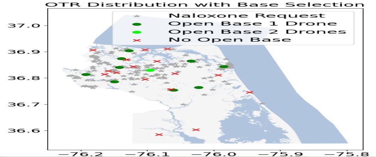
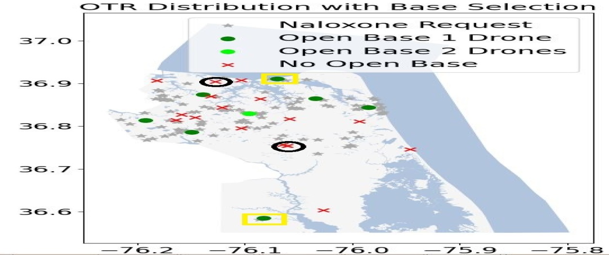
We now illustrate the spatio-temporal variability of the OTRs and its impact on the optimal configuration of the drone network. Figure 1 presents the distribution of the OTRs and drone networks for two consecutive quarters, i.e., 2018’s second (2018Q2) and third (2018Q3) quarters. In both networks, ten DBs are opened; one drone is located at nine of the DBs operating as systems while the last one operates as an system with two available drones. Comparing the two networks, one can see that the location of most DBs remains unchanged over time. One noticeable change is that, in the 2018Q3 network a new DB is opened in the southwest to cover an increased number of OTRs in this remote area. Another change is the new DB in the North. In Figure (1(b)), the two new DBs are surrounded by a rectangle while the two closed ones are circled. The location changes reflect the impact of the spatial uncertainty on the optimal configuration of the network. In that regard, the flexibility, ease, and limited cost to open (close) DBs [76] are important to adapt to geographical changes in the occurrence of OTRs.
6.2.3 Impact on Probability of Survival
The goal of this section is to quantify the benefits of the reduced response time afforded by the drone network (Section 6.2.2) on the survival chance of overdose victims. Since we are not aware of any functional relationship between response time and survival probability of an opioid overdose victim, we hereby employ an indirect two-step approach using known survival functions for cardiac arrests. The main reason for this is that many overdoses lead to cardiac arrests. Indeed, the increase in cardiac arrest caused by opioid medications is said to be “the most dramatic manifestation of opioid use disorder” [28].
Step 1: We calculate the number of out-of-hospital cardiac arrests (OHCA) due to opioid overdoses using the statistics reported by [28] [28] who indicate that 15% of opioid overdoses lead to an OHCA. As shown in Table 10, 560 overdose incidents are reported in Virginia Beach over one year (i.e., from 2018Q3 to 2019Q2), leading to an estimated (see [28]) number of 84 overdose-associated OHCAs.
Step 2: Using three known survival functions for OHCAs (see Table 3) that define the survival probability to an OHCA as either a semi-continuous or a logistic function of the response time , we calculate the estimated probability of survival for overdose-associated OHCAs with the drone network and with the EMS ambulance network in use in Virginia Beach. This allows us in turn to derive the differences in the survival chance and in the expected number of saved lives with the drone and ambulance networks.
| Author | Function Type | |
| Bandara et al. [4] | Semi-continuous | |
| De Maio et al. [27] | Logistic | |
| Chanta et al. [22] | Logistic |
Figure 2 shows the average survival probability – for the three survival functions in Table 3 – of the overdose-associated OHCAs obtained with the drone and with Virginia Beach’s ambulance-based EMS network. The survival probability reported in Figure 2 is the average of the survival probability of each OTR in the testing set from 2018Q3 to 2019Q2 in Table 2. The difference between the two networks is striking. The drone network significantly increases the patients’ survival probability. Indeed, the survival chance with the drone network is 3.54 (resp., 4.00 and 2.73) times larger than the one with Virginia Beach’s ambulance network as estimated by the survival function [4] (resp., [27], and [22]).
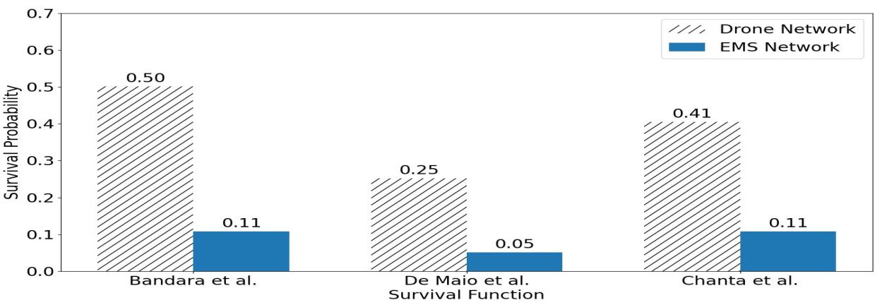
Table 4 displays the survival probability and the expected number of patients surviving an overdose-associated OHCA in Virginia Beach for the four quarters considered. These statistics are provided for the drone network (column 4) and for Virginia Beach’s ambulance network (column 5). One can see that the drone network is extremely beneficial and increases the number of survivors by 366%, (resp., 425% and 278%) using the survival function [4] (resp.[27] and [22]).
| Total Number | Overdose-related | Survival | Survival Prob. / No. of Survivors | |
| of Overdoses | OHCAs | Function | Drone Network | EMS Network |
| 560 | 84 | Bandara et al. [4] | 50% / 42 | 11% / 9 |
| De Maio et al. [27] | 25% / 21 | 5% / 4 | ||
| Chanta et al. [22] | 41% / 34 | 11% / 9 | ||
Table 4 shows that, depending on the survival function, the number of additional lives saved thanks to the drone network would vary between 17 and 33 in Virginia Beach over a one-year period of time. This is quite a striking result and is most likely an underestimate of the actual number of lives that could be saved with the drone network. Indeed, the above results only take into account the benefits of the drone-based reduced response time for the estimated percentage (15%) of opioid overdoses leading to a cardiac arrest. It is reasonable to assume that the reduced response time will also affect the outcomes of the overdoses not leading to a cardiac arrest, as underlined by [64] [64] who state that: ”Every minute that goes by before paramedics or others can attempt resuscitation, an opiate overdose victims’ chance of survival decreases by 10 percent”.
6.2.4 Impact on Quality-adjusted Life Year and Cost Analysis
The quality-adjusted life year (QALY) is a concept commonly used in healthcare economic analysis to evaluate how a healthcare issue impacts a survivor’s quality and duration of future life (see, e.g., [10, 71]). A QALY equal to 1 is indicative of one year in perfect health. As shown in (24), the total QALY (T-QALY) for a patient surviving a healthcare problem is the sum of the discounted QALY of each year during one’s mean life expectancy after the healthcare incident [10]:
| (24) |
where is the number of years of remaining life expectancy, is a coefficient accounting for the reduced quality of life consecutive to the healthcare incident, and is a discount rate reflecting that people prefer good health sooner than later (i.e., a QALY in earlier years is more valuable than in later ones).
To conduct the QALY analysis, we assume, as in [10], that a patient surviving an overdose-associated OHCA has a mean life expectancy of 11.4 years ( = 11.4), that each year corresponds to QALY (), and that the discount rate is 3%. Using (24), the T-QALY is equal to 8.47 years for each OHCA survivor (see Table 13 in Appendix M).
Table 5 presents the additional QALY gained by using drones instead of ambulances for the survival functions [4], [27], and [22] (see Table 3). The additional QALY attributable to the drone network for the overdose-associated OHCAs in Virginia Beach over one year is very high, varying between 143 and 279 years among the three survival functions.
| T-QALY | Survival | Number of Survivors | Additional Survivors | Additional QALY | |
| Function | Drone Network | EMS Network | with Drone Network | over one year | |
| 8.47 | Bandara et al. [4] | 42 | 9 | 33 | 279 |
| De Maio et al. [27] | 21 | 4 | 17 | 143 | |
| Chanta et al. [22] | 34 | 9 | 25 | 211 | |
A drone and the accompanying DB are estimated to cost , to have a four-year lifespan, and to have an annual maintenance cost of [10]. Using these statistics (see Table 14 in Appendix M), the total discounted costs of the eleven drones used in the base scenario amount to (i.e., using a 3% discount rate for the annual maintenance cost) and the drone-based network allows a reduction in the average response time of about 7 minutes and 16 seconds as compared to the ambulance network. That is quite a difference with the option of buying ambulances, each costing between $150,000 to $200,000, which, as stated by [64]. [64] would cost “millions and millions of dollars just to reduce the response time by a minute” (i.e., from eight to seven).
Assuming that the number of overdoses in Virginia Beach remains stable, the total additional QALY in four years (i.e., lifespan of a drone) attributable to the drone network reaches 1116, (resp., 572 and 844) years with the survival function [4] (resp., [27], and [22]), which in turn implies that the proposed drone network only costs $257 (resp., $503 and $341) per incremental QALY. As a benchmark, [10] [10] report a $3143 cost per incremental QALY for a network of drones delivering defibrillators to OHCAs in Durham, NC. More generally, it is considered that a medical intervention with a $50,000 per QALY ratio is cost-effective [62].
6.3 Comparison with Alternative Approaches
The results in the preceding section show that the drone network considerably reduces the average response time and increases the chance of survival of overdosed patients as compared to the ambulance-based EMS network in Virginia Beach. This is due, in part, to the fact that drones are not hindered by traffic and can reach the overdose incidents faster than ambulances. We investigate next to which extent the proposed drone network modelling and algorithmic technique contributes to the reduction in response time. We compare the results of our approach to those obtained with two constructive greedy heuristics (Section 6.3.1) and with a drone-network optimization model from the literature [15] (Section 6.3.2).
6.3.1 Comparison with Constructive Greedy Heuristics
In this section, we implement two constructive greedy heuristics (see, e.g., [30, 38, 41] and compare the networks obtained with these heuristics with the one constructed with our approach.
Description: The first heuristic, referred to as H-OTR, focuses on the number of overdoses at each OTR location and ranks the locations in a decreasing order by overdose occurrence (arrival) rate. The location ranked one is the one which has the largest occurrence rate of overdoses. We create two lists including respectively the OTR locations and the DB candidate locations and we update the lists at each step.
The heuristic H-OTR proceeds as follows. At each step, a new DB is opened. At first, we consider the OTR location with the largest overdose occurrence rate (i.e., ranked one) and we open a DB at the candidate location which is closest to the highest-ranked OTR location. This OTR location and the selected DB location are then removed from their respective lists. At each subsequent step, we consider the highest-ranked OTR location remaining in the list and open a DB at the closest candidate location. The addition of DBs stops when the number of DBs that can be opened is attained. If some drones are left, i.e., instances in which the number of drones is larger than the number of DBs that can be opened, we place a second drone at the DB(s) opened first. The pseudo-code of H-OTR is in Appendix K.
The second heuristic, referred to as H-DB, focuses on the proximity of the DB candidate locations from the overdose incidents. Instead of operating on a ranking of the overdose locations as in H-OTR, the H-DB heuristic ranks the DB candidate locations. The DB candidate location ranked first is the one with the largest potential demand, i.e., largest number of overdose incidents, within the catchment area of a drone positioned at this DB. As before, we create and update at each step of the heuristic two lists including respectively the OTR locations and the DB candidate locations. The heuristic H-DB proceeds as follows. At each step, a new DB is opened. At first, we consider the DB candidate location with the largest demand and we open a DB there. After each iteration, the selected DB and the OTR locations closest to it are removed from the candidate sets considered at the subsequent iterations. A new ranking is then recalculated for the DB candidate locations based on the remaining (udpated) list of OTR locations. The greedy addition of DBs stops when the number of DBs that can be opened is attained. As for H-OTR, if the number of available drones is larger than the number of DBs, we place a second drone at the DB(s) opened first, i.e., those with the highest arrival rate. The pseudo-code of H-DB is in Appendix K.
Results and Comparison: We now compare the network built with our approach and model R-MILP with the two networks built using the heuristics H-OTR and H-DB respectively. We proceed as follows. First, we run the heuristics H-OTR and H-DB and solve R-MILP to obtain the location of the opened DBs and the number of drones positioned at each DB with each approach. Second, we run the simulation 100 times for each of the three networks built with H-OTR, H-DB, and R-MILP. For each, we record two types of response times from the simulation. First, we record the average network-wide response time (i.e., average across all OTRs). Second, for each OTR , we record the average response time across the 100 simulations. The results described next attest the superior performance of the network built with our model R-MILP. The advantages of the R-MILP-based network over those constructed with the heuristics are twofold. First, the R-MILP-based network reduces significantly the average response time . Table (7) shows that the average response time of the R-MILP network is 36.02% and 46.78% lower than the average response time with the H-DB- and H-OTR-based networks, respectively.
| Training Set | Average Network-wide | R-MILP Time Reduction | |||
| Response Time (minutes) | with respect to: | ||||
| H-DB | H-OTR | R-MILP | H-DB | H-OTR | |
| 2018Q2 | 2.29 | 2.75 | 1.49 | 34.93% | 45.82% |
| 2018Q3 | 2.29 | 3.70 | 1.58 | 31.00% | 57.30% |
| 2018Q4 | 2.49 | 2.31 | 1.54 | 38.15% | 33.33% |
| 2019Q1 | 2.48 | 2.72 | 1.50 | 39.52% | 44.85% |
| Average | 2.39 | 2.87 | 1.53 | 36.02% | 46.78% |
Second, the R-MILP-based network also reduces considerably the upper tail of the distribution of the average OTR response time . Figure 6 (in Appendix L) displays the distribution of the average response time for the R-MILP-, H-OTR-, and H-DB-based networks. As it can be clearly seen, the R-MILP-based network does not only lessen the average response time (red solid line), but also significantly reduces the gap, i.e., time difference, between the average response time and the 90th quantile of the response time (red dashed line). The narrower gap is indicative of a more equitable EMS system since the response time exhibits less variability among all OTRs.
As few seconds can be the difference between life and death in the context of opioid overdoses [64], the value of our model becomes evident and explains why Buckland et al. [18] urge, in regards to using drones for medical emergencies, to develop advanced resource allocation and optimization algorithms.
6.3.2 Comparison with Alternative Drone Delivery Model
To show the added benefit of our modeling approach, referred to as R-MILP, we build a benchmark network using the optimization model proposed in [15] in which drones are utilized to deliver automated external defibrillators to people having out-of-hospital cardiac arrests. We refer thereafter to this model with the acronym BM short for benchmark model. At a high level, the model BM seeks to minimize the total number of drones to be deployed while ensuring that the average response time of the drone network is at least minutes shorter (i.e., is a parameter fixed a priori) than the current EMS system. Using the data from the second quarter of 2018, we set minutes – which is the time improvement targeted in [15] – in model BM. We carry out the simulation process 100 times using the optimal DB locations and number of drones determined by the optimal solutions of the two models BM and R-MILP. For each simulation run in each model, we record the mean network-wide response time across all OTRs. Table 8 reports the statistics for the network-wide response time based on 100 simulations.
| Summary Statistics | Response Time (minutes) | ||
| BM | R-MILP | Time Reduction | |
| 5th Percentile | 5.48 | 0.80 | 85% |
| Average | 6.67 | 1.49 | 78% |
| 95th Percentile | 8.03 | 2.19 | 73% |
Clearly, the network based on the R-MILP model is much superior to the one based on the BM model as the average response time with the R-MILP model is 78% lower than with the BM model. The average response time with our model R-MILP is one minute and 29 seconds while the average response-time with the BM model is six minutes and 40 seconds. Similarly, the 5th and 95th response time percentiles with the R-MILP model are respectively 85% and 73% lower than those with the BM model. The results in Table 8 are unequivocal about the superiority and the advantages offered by the model constructed with our model R-MILP. The response time gain is crucial in view of how a few seconds can be the difference between life and death in this context.
6.4 Computational Efficiency
In this section, we conduct a battery of tests to assess the computational efficiency and tractability of the proposed reformulation and algorithms. Section 6.4.1 compares the two proposed algorithms and the direct solution of the reformulated problem with Gurobi. Performance profile plots [29] highlight the increased benefits gained with our approaches as the size of the problem and the volume of OTRs increases. Section 6.4.2 assess the sensitivity of the proposed method with respect to available resources.
All formulations are coded in Python 3.7 and solved with the Gurobi solver on a Linux machine, with Intel Core i7-6700 CPU 3.40GHz processors and 64 GB installed physical memory. For each instance, the optimality tolerance is 0.01%, the maximum solution time is one hour, and we use one thread only.
6.4.1 Computational Efficiency of Scalability
We evaluate here the computational efficiency and scalability of the proposed reformulations L-MILP, R-MILP and algorithms with respect to the size of the problem, namely the number of OTRs to which the network must respond. Using the data described in Section 6.1 and considering the base network scenario with up to 10 DBs and 11 drones, we have created ten problem types that differ in the number of OTRs ranging from 50 to 500, by increment of 50: . Each instance type is identified by the tuple and we have generated five problem instances for each instance type. This gives a total of 50 instances which we solve with the following approaches:
-
•
REFO: Direct solution of the larger-size MILP problem L-MILP (15) with the default settings of the Gurobi solver.
-
•
OA: Outer approximation algorithm (Remark 3) with model L-MILP.
-
•
OA-B&C: Outer Approximation branch-and-cut algorithm with model L-MILP.
-
•
R-OA-B&C: Outer Approximation branch-and-cut algorithm with model R-MILP.
The four approaches are compared in terms of solution times and the number of instances for which optimality can be proven in one hour. We note that none of the 50 problem instances formulated with the base formulation B-IFP can be solved in one hour with the state-of-the-art solver Baron specialized for nonconvex MINLP problems. We use performance profile plots displayed in Figure (3(a)) to compare the efficiency of the solution methods. The horizontal axis indicates the running time in seconds while the vertical axis represents the number of instances solved to optimality within the corresponding running time. The solution time for each instance is given in Table 15 in Appendix N.
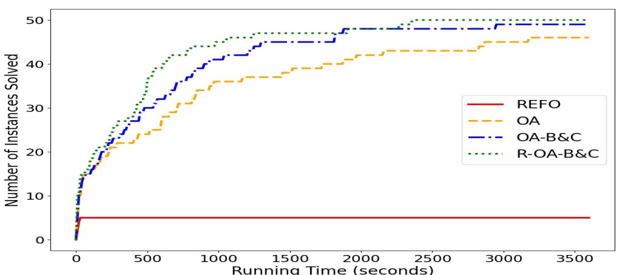
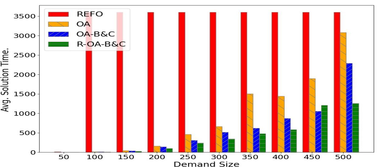
The performance profile shows clearly that the proposed methods OA, OA-B&C and R-OA-B&C are much faster, scale much better, and allow the solution of many more instances than the direct solution method REFO. While the direct solution approach REFO only solves five (i.e. the five smallest instances with = 50 OTRs) of the 50 instances in one hour, OA, OA-B&C, and R-OA-B&C solve and prove the optimality of the solution for respectively 46, 49, and 50 instances. Comparing now the algorithms OA and OA-B&C, the dynamic incorporation of valid inequalities and optimality cuts leads to further efficiency and scalability gains. This can be seen from the OA-B&C line in the performance plot being above the OA line at any time interval, thereby indicating that the OA-B&C method solves more instances to optimality in any amount of time. As an illustration, Table 16 in Appendix shows that OA-B&C solves 96% of the instances in less than 40 minutes while OA needs one hour to solve 92% of the instances.
The solution method R-OA-B&C based on the B&C outer approximation method and the compact MILP reformulation R-MILP improves further the solution process over OA-B&C. The performance profile of R-OA-B&C is systematically above that of OA-B&C. which shows that, in any considered amount of time, R-OA-B&C is able to solve more instances than OA-B&C, and demonstrates the computational benefits provided by the compact MILP reformulation R-MILP. For instance, while OA-B&C solves 64% of the instances to optimality in 600 seconds, R-OA-B&C does so for 78% of them in the same time.
Figure (3(b)) shows the average (across five instances) solution times for each instance type and associated size . When an instance cannot be solved to optimality within one hour, the solution time is estimated to be 3600 seconds, which explains that for all instances of size the solution time for REFO is 3600 seconds. Figure (3(b)) highlights the added benefits of R-OA-B&C over OA-B&C and OA for larger instances. While R-OA-B&C (green bar), OA-B&C (blue bar), and OA (orange bar) perform similarly for , R-OA-B&C and OA-B&C solve the instances of larger size much faster than OA can do. It can be seen that OA and OA-B&C take respectively 140% and 80% more time than R-OA-B&C to solve the 500-sized instances.
6.4.2 Sensitivity Analysis with Respect to Network Resources
In this section, we evaluate the sensitivity of the solution times with respect to the resources of the network and, in particular the number of DBs () and drones (). We use the algorithm R-OA-B&C since it enjoys the quickest solution time as shown in Section 6.4.1.
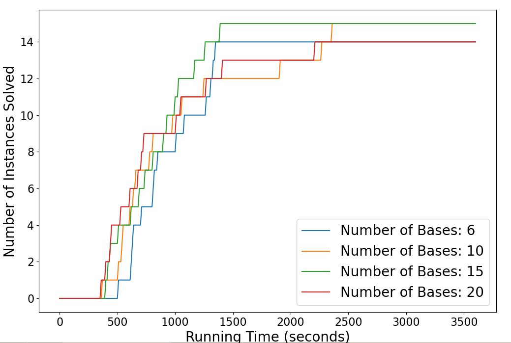
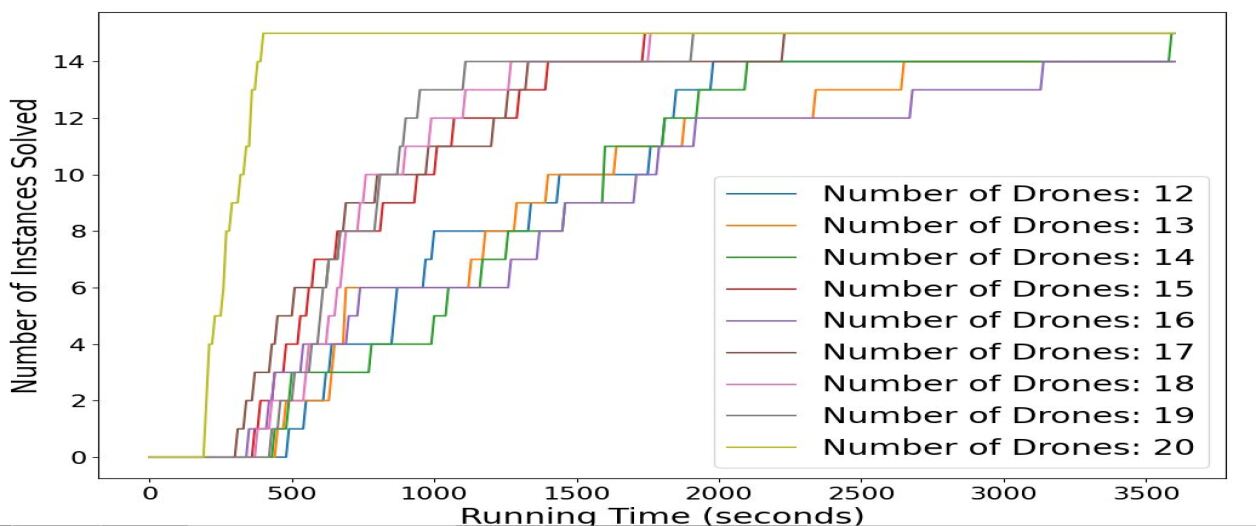
We consider four possible values for the number of DBs and three values for the demand size (number of OTRs), and generate for each combination of and five problem instances. We assume that drones are available. This gives 12 instance types for a total of 60 problem instances and we solve each of these with the R-OA-B&C algorithm. Figure (4(a)) shows the performance profile associated to each considered number of DBs. It appears that the computational time of the R-OA-B&C method is not particularly sensitive to the number of open DBs since the performance profiles for the considered values of intersect, thereby indicating the solution time is not systematically higher (or lower) for any considered number of DBs.
We proceed similarly to evaluate the sensitivity of the computational time with respect to the number of drones. We assume that the maximum number of DBs that can be open is . We consider nine possible number of available drones , three possible demand sizes , and generate five instances for each of the 27 instance types of each type for a total of 135 instances that we solve with the R-OA-B&C method. The corresponding performance profile in Figure 4(b) shows that the solution process tends to be quicker (i.e. more instances solved in a given amount of time) when the number of available drones is larger. We notice in particular that the average solution time is much lower for than for any other (smaller) value assigned to .
7 Conclusions
Opioid use affects about 2 million Americans and cost $78.5 billion in annual health care expenses [28]. It has been argued that the drone-based delivery of naloxone has the “potential to be a transformative innovation due to its easily deployable and flexible nature” [36]. The efficacy of naloxone depends on how quickly it is administered, which is a priority of the US Food and Drug Administration [64].
This study responds to the above pressing needs and proposes a new queueing-optimization model to design an EMS network in which drones deliver naloxone to overdose victims in a timely fashion. The objective is to increase the chance of survival of overdose victims by reducing the time needed to deliver and administer naloxone and is accomplished by determining the location of drones and DBs, the capacity of DBs, and the dispatching of drones to overdose incidents. Some new distinctive features in the model are its survival objective function, the explicit modeling of congestion and decision-dependent (parameter) uncertainty in the service time that affects the performance of the network, and its flexibility as the capacity of DBs is not fixed ex-ante but is instead determined by the model.
Besides modeling, the contributions of this study are threefold. On the reformulation side, we propose a tractable MILP reformulation of the stochastic network design problem, which, in its original form, is a fractional integer optimization problem. We further demonstrate the generalizability of the reformulation approach and prove that the problem of minimizing the average network-wide response time of a collection of interdependent queueing systems in which the capacity of each system is variable is MILP-representable. On the algorithmic side, we design an outer approximation branch-and cut algorithmic framework which is a significant upgrade over the direct solution of the MILP reformulations. The algorithm, in particular when used with the reduced-size MILP reformulation, significantly reduces the solution time, increases the number of solved instances, and enables the solution of problems of larger size than those encountered in our case study. On the EMS practice side, the tests based on real-life data from Virginia Beach reveal that the use of drones to deliver naloxone in response to overdoses could possibly be a game-changer. Besides showing the out-of-sample robustness and applicability of the proposed approach, the tests attest that using the drone network: 1) the response time is on average (1 min and 39 sec) close to seven times smaller than the one (9 min and 19 sec) with the ambulance network used in Virginia Beach; 2) the estimated chance of survival to an overdose is more than 2.73 times larger than the one with the Virginia Beach ambulance network; 3) many more lives (of overdose victims) could be saved; 4) the total QALY per patient is 8.47 years amounting to up to 279 additional per year across all overdose victims in Virginia Beach; 5) the cost per additional QALY is very low, varying between $257 and $502; and 6) one can markedly decrease the response time and increase the survival chance as compared to using heuristics and an alternative model from the literature.
This study showcases the potential of using drones to alleviate the devastating consequences of the opioid overdose crisis and could pave the way for the practical implementation of drone-based EMS systems. While very promising, we must however be aware of a number of obstacles for the widespread use of drones to respond to overdoses or other time-critical medical emergencies. These barriers include, for example, regulation, flying condition and zones, safety, data privacy, operations related to the design and maintenance of a medical drone network [43]. While not the focus of this study, future research will be needed to investigate these hindrances as well as user perceptions and acceptance.
References
- [1] Robert Aboolian, Oded Berman and Zvi Drezner “Location and allocation of service units on a congested network” In IIE Transactions 40.4 Taylor & Francis, 2008, pp. 422–433
- [2] Warren P Adams and Richard J Forrester “Linear forms of nonlinear expressions: Newinsights on old ideas” In Operations Research Letters 35, 2007, pp. 510–518
- [3] A. Atamtürk and V. Narayanan “Polymatroids and Mean-risk Minimization in Discrete Optimization” In Operations Research Letters 36.5, 2008, pp. 618–622
- [4] D. Bandara, M.E. Mayorga and L.A. McLay “Priority dispatching strategies for EMS systems” In Journal of the Operational Research Society 65.4, 2014, pp. 572–587
- [5] Rajan Batta and Oded Berman “A location model for a facility operating as an M/G/k queue” In Networks 19.6 Wiley Online Library, 1989, pp. 717–728
- [6] J. Bauer, D. Moormann, R. Strametz and D.A. Groneberg “Development of Unmanned Aerial Vehicle Networks Delivering Early Defibrillation for Out-of-Hospital Cardiac Arrests in Areas Lacking Timely Access to Emergency Medical Services in Germany: A Comparative Economic Study” In BMJ Open 11, 2021, pp. 1–7
- [7] O. Berman and D. Krass “Stochastic Location Models with Congestion” In Location Science Springer, 2019, pp. 477–535
- [8] Oded Berman and Zvi Drezner “The multiple server location problem” In Journal of the Operational Research Society 58.1 Taylor & Francis, 2007, pp. 91–99
- [9] Oded Berman, Richard C Larson and Samuel S Chiu “Optimal server location on a network operating as an M/G/1 queue” In Operations Research 33.4 INFORMS, 1985, pp. 746–771
- [10] Brittany Bogle, Wayne Rosamond, Kyle Snyder and Jessica Zègre-Hemsey “The Case for Drone-assisted Emergency Response to Cardiac Arrest: An Optimized Statewide Deployment Approach” In North Carolina Medical Journal 80, 2019, pp. 204–212 DOI: 10.18043/ncm.80.4.204
- [11] J.S. Borrero, C. Gillen and O.A. Prokopyev “A Simple Technique to Improve Lineraized Reformulations of Fractional (hyperbolic) 0-1 Programming Problems” In Operations Research Letters 44, 2016, pp. 479–486
- [12] J.S. Borrero, C. Gillen and O.A. Prokopyev “Fractional 0-1 Programming: Applications and Algorithms” In Journal of Global Optimization 69.1, 2017, pp. 255–282
- [13] J. Boutilier et al. “Optimizing a drone network to deliver automated external defibrillators” In Circulation 135.25 Am Heart Assoc, 2017, pp. 2454–2465
- [14] J. Boutilier and Timothy C.Y. Chan “Ambulance Emergency Response Optimization in Developing Countries” In Operations Research 68.5, 2020, pp. 1315–1334 DOI: 10.1287/opre.2019.1969
- [15] J. Boutilier and Timothy C.Y. Chan “Drone Network Design for Cardiac Arrest Response” In Manufacturing & Service Operations Management 24.5, 2022, pp. 2407–2424
- [16] A. Brill and B. Ganz “The Geographic Variation in the Cost of the Opioid Crisis”, 2018
- [17] J.J.M. Bront, I Mendez-Díaz and G. Vulcano “A column generation algorithm for choice-based network revenue management” In Operations Research 57, 2009, pp. 769–784
- [18] D.M. Buckland et al. “Design Considerations for UAV-Delivered Opioid Overdose Interventions” In 2019 IEEE Aerospace Conference, 2019, pp. 1–7
- [19] Centers for Disease Control and Prevention “Opioid Overdose” [Online; accessed February 19, 2022], https://www.cdc.gov/drugoverdose/opioids/index.html
- [20] Centers for Disease Control and Prevention “Overdose Deaths Accelerating During COVID-19” [Online; accessed August 19, 2021], https://www.cdc.gov/media/releases/2020/p1218-overdose-deaths-covid-19.html
- [21] Centers for Disease Control and Prevention “Understanding the Epidemic” [Online; accessed August 19, 2021], https://www.cdc.gov/opioids/basics/epidemic.html
- [22] S. Chanta, M.E. Mayorga and L.A. McLay “The minimum p-envy location problem with requirement on minimum survival rate” In Computers and Industrial Engineering 74, 2014, pp. 228–239
- [23] Sheldon Cheskes et al. “Improving access to automated external defibrillators in rural and remote settings: A drone delivery feasibility study” In Journal of the American Heart Association 9.14, 2020, pp. e016687
- [24] Samuel S. Chiu and Richard C. Larson “Locating an n-server facility in a stochastic environment” In Computers & Operations Research 12.6, 1985, pp. 509–516
- [25] Y. Crama and E. Rodrıguez-Heck “A class of valid inequalities for multilinear 0–1 optimization problems” In Discrete Optimization 25, 2017, pp. 28–47
- [26] J. Custodio and M.A. Lejeune “Spatiotemporal Data Set for Out-of-Hospital Cardiac Arrests” In INFORMS Journal on Computing 34.1, 2022, pp. 4–10
- [27] V.J. De Maio et al. “Optimal Defibrillation Response Intervals for Maximum Out-of-Hospital Cardiac Arrest Survival Rates” In Annals of Emergency Medicine 42, 2003, pp. 242–250
- [28] C. Dezfulian et al. “Opioid-Associated Out-of-Hospital Cardiac Arrest: Distinctive Clinical Features and Implications for Health Care and Public Responses: A Scientific Statement From the American Heart Association” In Circulation 143.16, 2021, pp. e836–e870
- [29] E.D. Dolan and J.J. Moré “Benchmarking Optimization Software with Performance Profiles” In Mathematical Programming 91, 2002, pp. 201–213
- [30] Daryna Dziuba and Christian Almeder “New construction heuristic for capacitated lot sizing problems” In European Journal of Operational Research 311, 2023, pp. 906–920
- [31] S. Elhedhli “Exact solution of a class of nonlinear knapsack problems” In Operations Research Letters 33, 2005, pp. 615–624
- [32] E. Erkut, A. Ingolfsson and G. Erdogan “Ambulance Location for Maximum Survival” In Naval Research Logistics 55, 2008, pp. 42–58
- [33] Lanah Evers, Ana Isabel Barros, Herman Monsuur and Albert Wagelmans “Online stochastic UAV mission planning with time windows and time-sensitive targets” In European Journal of Operational Research 238, 2014, pp. 348–362
- [34] A. Fischer, F. Fischer and S.T. McCormick “Matroid optimisation problems with nested non-linear monomials in the objective function” In Mathematical Programming 169, 2018, pp. 417–446
- [35] R. Fortet “Applications de l’Algèbre de Boole en Recherche Opérationnelle” In Revue Française d’Automatique, d’Informatique et de Recherche Opérationnelle 4, 1959, pp. 5–36
- [36] X. Gao, N. Kong and P.M. Griffin “Dynamic optimization of drone dispatch for substance overdose rescue” In 2020 Winter Simulation Conference (WSC), 2020, pp. 830–841 IEEE
- [37] J.C. Góez and M.F. Anjos “Second-order cone optimization formulations for service system design problems with congestion” In Modeling and Optimization: Theory and Applications Springer, 2017, pp. 97–120
- [38] Harsha Gwalani, Chetan Tiwari and Armin Mikler “Evaluation of Heuristics for the P-Median Problem: Scale and Spatial Demand Distribution” In Computers, Environment and Urban Systems 88, 2021, pp. 101656
- [39] J. Han, K. Lee, C. Lee and S. Park “Exact algorithms for a bandwidth packing problem with queueing delay guarantees” In INFORMS Journal on Computing 25, 2013, pp. 585–596
- [40] L. Hellemo, P. Barton and A. Tomasgard “Decision-dependent probabilities in stochastic programs with recourse” In Computational Management Science, 2018, pp. 369–395
- [41] Gerbrich Hoekstra and Frank Phillipson “Heuristic Approaches for Location Assignment of Capacitated Services in Smart Cities” In Journal of Computers 7, 2018, pp. 67
- [42] L’udmila Jánošı́ková, Peter Jankovič, Marek Kvet and Frederika Zajacová “Coverage versus response time objectives in ambulance location” In International Journal of Health Geographics 20.1, 2021, pp. 1–16
- [43] A.M. Johnson et al. “Impact of Using Drones in Emergency Medicine: What Does the Future Hold?” In Open Access Emergency Medicine 2021:13 Dovepress, 2021, pp. 487–498
- [44] Todd Kerensky and Alexander Walley “Opioid overdose prevention and naloxone rescue kits: What we know and what we don’t know” In Addiction Science & Clinical Practice 12, 2017
- [45] T. Kleinert, V. Grimm and M. Schmidt “Outer approximation for global optimization of mixed-integer quadratic bilevel problems” In Mathematical Programming, 2021, pp. 1–61
- [46] M.A. Lejeune and F. Margot “Drone Response to Out-of-Hospital Cardiac Arrests”, Working Paper, 2022
- [47] H.-L. Li “A Global Approach for General 0–1 Fractional Programming” In European Journal of Operational Research 73.3, 1994, pp. 590–596
- [48] Y.H. Lin and Q. Tian “Exact approaches for competitive facility location with discrete attractiveness” In Optimization Letters 15, 2021, pp. 377–389
- [49] A. Lundell and J. Kronqvist “Integration of polyhedral outer approximation algorithms with MIP solvers through callbacks and lazy constraints” In AIP Conference Proceedings 2070.1, 2019, pp. 020012 AIP Publishing LLC
- [50] Rachael Lynn and Jeffrey Galinkin “Naloxone dosage for opioid reversal: Current evidence and clinical implications” In Therapeutic Advances in Drug Safety 9, 2017, pp. 204209861774416
- [51] C. Mackle et al. “A Data-Driven Simulator for the Strategic Positioning of Aerial Ambulance Drones Reaching Out-of-Hospital Cardiac Arrests: A Genetic Algorithmic Approach” In IEEE Journal of Translational Engineering in Health and Medicine 8, 2020, pp. 1–10
- [52] V. Marianov and C. Revelle “The queueing maximal availability location problem: A model for the siting of emergency vehicles” In European Journal of Operational Research 93.1, 1996, pp. 110–120
- [53] V. Marianov and C. Revelle “The queuing probabilistic location set covering problem and some extensions” In Socio-Economic Planning Sciences 28.3, 1994, pp. 167–178
- [54] Vladimir Marianov and Daniel Serra “Location–Allocation of Multiple-Server Service Centers with Constrained Queues or Waiting Times” In Annals of Operations Research 111, 2002, pp. 35–50
- [55] R. McCormack and G. Coates “A Simulation Model to Enable the Optimization of Ambulance Fleet Allocation and Base Station Location for Increased Patient Survival” In European Journal of Operational Research 247, 2015, pp. 294–309
- [56] Garth P McCormick “Computability of global solutions to factorable nonconvex programs: Part I—Convex underestimating problems” In Mathematical programming 10.1 Springer, 1976, pp. 147–175
- [57] Jyotiprasad Medhi “Stochastic models in queueing theory” Elsevier, 2002
- [58] Erfan Mehmanchi, Andrés Gómez and Oleg A. Prokopyev “Fractional 0–1 programs: links between mixed-integer linear and conic quadratic formulations” In Journal of Global Optimization 75.2, 2019, pp. 273–339
- [59] M.I. Mermiri, G.A. Mavrovrounis and I.N. Pantazopoulos “Drones for Automated External Defibrillators Delivery: Where do we Stand?” In Journal of Emergency Medicine 59, 2020, pp. 660–667
- [60] A. Mills, N. Argon and S. Ziya “Resource-based patient prioritization in mass-casualty incidents” In Manufacturing & Service Operations Management 15, 2013, pp. 361–377
- [61] M. Moshref-Javadi and M. Winkenbach “Applications and Research Avenues for Drone-based Models in Logistics: A Classification and Review” In Expert Systems with Applications 177, 2021, pp. 114854
- [62] P.J. Neumann, J.T. Cohen and M.C. Weinstein “Updating Cost-Effectiveness— The Curious Resilience of the $50,000-per-QALY Threshold” In New England Journal of Medicine 371.9, 2014, pp. 796–797
- [63] Shirley A. Nozaki and Sheldon M. Ross “Approximations in finite-capacity multi-server queues by Poisson arrivals” In Journal of Applied Probability 15.4 Cambridge University Press, 1978, pp. 826–834 DOI: 10.2307/3213437
- [64] J.P. Ornato et al. “Feasibility of bystander-administered naloxone delivered by drone to opioid overdose victims” In The American Journal of Emergency Medicine 38.9, 2020, pp. 1787–1791
- [65] O.A. Prokopyev, H.-X. Huang and P.M. Pardalos “On Complexity of Unconstrained Hyperbolic 0-1 Programming Problems” In Operations Research Letters 33.3, 2005, pp. 312–318
- [66] N. Pulsiri, R. Vatananan-Thesenvitz, T. Sirisamutr and P. Wachiradilok “Save Lives: A review of ambulance technologies in pre-hospital emergency medical services” In PICMET 2019 - Portland International Conference on Management of Engineering and Technology: Technology Management in the World of Intelligent Systems, 2019, pp. 1419–1428
- [67] Aaron Pulver and Ran Wei “Optimizing the spatial location of medical drones” In Applied Geography 90, 2018, pp. 9–16
- [68] Aaron Pulver, Ran Wei and Clay Mann “Locating AED enabled medical drones to enhance cardiac arrest response times” In Prehospital Emergency Care 20.3 Taylor & Francis, 2016, pp. 378–389
- [69] Sheldon Ross “Chapter 8 - Queueing Theory” In Introduction to Probability Models (Eleventh Edition) Boston: Academic Press, 2014, pp. 481–558
- [70] J. Rosser, V. Vignesh, B. Terwilliger and B. Parker “Surgical and Medical Applications of Drones: A Comprehensive Review” In Journal of the Society of Laparoendoscopic Surgeons 22, 2018, pp. 1–9
- [71] F. Sassi “Calculating QALYs, Comparing QALY and DALY Calculations” In Health Policy Plan 21.5, 2006, pp. 402–408
- [72] Judy E Scott and Carlton H Scott “Models for drone delivery of medications and other healthcare items” In Unmanned Aerial Vehicles: Breakthroughs in Research and Practice IGI Global, 2019, pp. 376–392
- [73] A. Sen, A. Atamturk and P. Kaminsky “A conic integer optimization approach to the constrained assortment problem under the mixed multinomial logit model” In Operations Research 66.4, 2018, pp. 994–1003
- [74] Society of Actuaries “Economic Impact of Non-Medical Opioid Use in the United States” [Online; accessed August 19, 2021], https://www.soa.org/globalassets/assets/files/resources/research-report/2019/econ-impact-non-medical-opioid-use.pdf
- [75] Connor Tukel et al. “Time-to-scene for opioid overdoses: are unmanned aerial drones faster than traditional first responders in an urban environment?” In BMJ Innovations 6, 2020, pp. 204–208
- [76] Patrick Van de Voorde et al. “The drone ambulance [A-UAS]: Golden bullet or just a blank?” In Resuscitation 116 Elsevier, 2017, pp. 46–48
- [77] World Health Organization “Opioid Overdose” [Online; accessed August 19, 2021], https://www.who.int/news-room/fact-sheets/detail/opioid-overdose, 2020
- [78] J. Xu, A. Murray, R. Church and R Wei “Service allocation equity in location coverage analytics” In European Journal of Operational Research 305, 2023, pp. 21–37
- [79] J.J. Ye, C. Zhang, João Ricardo Nickenig Vissoci and D. Buckland “Optimizing a Drone Network to Deliver Naloxone” In Annals of Emergency Medicine 74, 2019, pp. S64
Appendix A Abbreviations
-
DB:
Drone base.
-
EMS:
Emergency medical services.
-
OHCA:
Out-of-hospital cardiac arrest.
-
OTR:
Overdose-triggered request.
-
QALY:
Quality-adjusted life year.
Appendix B Notations
B.1 Sets and Indices
-
:
Index and set of OTR locations.
-
:
Index and set of candidate DBs.
-
:
Index and set of OTRs that are within the catchment area of a drone at DB .
-
:
Index and set of DBs that can cover OTR .
-
:
Index and set of drones.
B.2 Parameters and Constants
-
:
Vector of parameters representing the coordinates of DB in the earth-centered, earth-fixed coordinate system.
-
:
Vector of parameters representing the location of OTR in the earth-centered, earth-fixed coordinate system.
-
:
Maximum number of drones that can be stationed at any DB.
-
:
Distance between OTR and candidate DB .
-
:
Flight speed of drones.
-
:
OTR arrival (occurrence) rate from at .
-
:
Maximal number of available drones.
-
:
Maximal number of drone bases that can can be established.
-
:
Coefficient modulating the travel speed to and from an OTR location.
-
:
Flight radius of a drone.
B.3 Decision Variables
-
:
Binary variable determining if a DB is open at candidate location () or not ().
-
:
Binary variable defining if OTR at location is assigned to open DB () or not ().
-
:
Binary variable indicating the number of drones deployed at DB : if and only if drones are positioned at DB .
-
:
General integer variable defining the number of drones stationed at DB .
-
:
Arrival rate of OTRs serviced by DB .
-
:
Auxiliary variable introduced to reformulate the fractional terms of the objective function.
-
:
Auxiliary variable introduced to linearize the bilinear term .
-
:
Auxiliary variable introduced to linearize the bilinear term .
-
:
Auxiliary variable introduced to linearize the bilinear term .
-
:
Auxiliary variable introduced to linearize the bilinear term .
B.4 Random Variables
-
:
Service time for OTR at if serviced with a drone stationed at DB .
-
:
Service time of a drone at DB .
-
:
Queueing delay time for DB .
-
:
Response time between reception of the delivery request and arrival of a drone for an OTR at .
-
:
On-scene service time (e.g. naloxone toolkit unloading time) for location .
-
:
Drone reset time needed to recharge and load new naloxone toolkit for location .
-
:
Non-travel drone service time equal to for OTR at location .
Appendix C Proofs
C.1 Proof of Proposition 1
Proposition 1: The functional form of the average response time is a fractional expression with nonlinear numerator and denominator:
C.2 Proof of Remark 2
Remark 2: Problem is a nonconvex optimization problem in which:
(i) The objective function is neither convex, nor concave: the denominator and the numerator in each ratio term of the objective function are nonconvex functions;
(ii) The ratio terms can involve division by 0 and be indeterminate;
(iii) Any ratio term related to a
location where no DB is set up in undefined;
(iv) There is a mix of binary and bounded general integer variables;
(v) The continuous relaxation of is a nonconvex problem.
Proof:
(i) The numerator and denominator include polynomial and exponential terms.
The denominator has also factorial and fractional terms. Both are nonconvex functions.
It can be easily shown that the hessian matrix of the fractional objective function is not positive semidefinite, nor negative semidefinite.
(ii) Any term can be equal to 0, which leads to a division by 0, if
no DB is set up at location , thereby implying .
(iii) If no DB is set up at the potential location , no drone can be stationed at , which implies that . In that case, the denominator includes a term involving taking the factorial of a negative number:
(iv) Obvious: see constraints (8h)-(8i).
(v) See part (i).
C.3 Proof of Proposition 2
Proposition 2: Let . The fractional nonlinear binary problem
| s.to | ||||
is equivalent to the fractional nonlinear integer problem .
Proof: Part (i): We first replace each bounded general integer variable by a weighted sum of binary variables in the constraints. For this substitution to work, (28) must hold:
| (28) |
This is accomplished in two steps. First, we introduce the linear constraints
| (29a) | ||||
| (29b) | ||||
for each (see (9e) and (9f)) to ensure that can take any integer value in which is the restriction imposed on each via (8f) and (8i). Accordingly, we substitute (9e)-(9f) for (8i) and then replace by the right-side term of (28) in (8b), (8f), and (8g). We divide both sides of (8b) by and substract the infinitesimal positive constant from the right side. The constraints (8b), (8f), and (8g) can then be replaced by (9b), (9c), and (9d) in the constraint set of . This gives the mixed-integer feasible set given in the statement of Proposition 2.
Part (ii): We now remove the general integer variables from the objective function (8a). In each term of the objective, we first replace the general integer variable by the index parameter , which gives:
| (30) |
Next, we multiply each expression (30) by the corresponding binary variable and we sum the resulting ratio terms (i.e., ), which gives
| (31) |
with () denoting the possible number of drones positioned at any open DB.
Due to (9e), at most one binary variable for each takes a non-zero value (i.e., 1) and, therefore, at most one term in the summation is (31) is non-zero. This, combined with the fact that the feasible set of ensures that (28) holds true for each (see Part i)), implies that (31) is equivalent to the expression in the second line of the objective function (8a) of B-IFP, as shown next.
Two cases are now to be considered. First, if for any arbitrary , we have , each is equal to 0 since the constraints in imply (28), and (31) is equal to 0. Second, if with , then exactly one of the is equal to 1. More precisely, due to (28), we have and . This means that the only term in (31) taking a non-zero value is the one for which , which in turn implies that each term in (31) is equal to the expression in the second line of (8a), which provides the result that we set out to prove.
C.4 Proof of Theorem 3
Theorem 3: Define the index sets . Let , , , and be continuous auxiliary variables used for the linearizization of bilinear terms. The MILP problem
| s.to | |||||
is equivalent to the nonlinear integer problems and for =2.
Proof: (i) Linearization: For , the fractional terms
| (33) |
in (9a) can be rewritten as
In order to remove the fractional terms from the objective function, we introduce the nonnegative auxiliary variables defined as:
| (34) | ||||
| (35) |
Problem R-BFP can now be equivalently rewritten as:
| (36) | ||||
| s.to | ||||
The second step is the linearization of the nonconvex equality constraints (34) and (35) and the polynomial terms of the objective function (36). Multiplying both sides of (34) by gives
| (37) |
which can be linearized as (13c) by introducing the linearization auxiliary variables and the McCormick inequalities in the set to ensure that: .
Similarly, multiplying both sides of (35) by
gives
| (38) |
The left-hand side of (38) can be rewritten as
| (39a) | ||||
| (39b) | ||||
The double summation expression in (39) can be simplified. First, using the idempotent identity of binary variables, we have: . Second, we split the summands in (39) into two parts including respectively the separable bilinear terms and the nonseparable ones :
| (40) |
Combining (39) and (40), we reformulate the left side of (38) as:
| (41) |
Using the same reasoning, the right-hand side of (38) is equal to
Thus, (35) and (38) are equivalent to
| (42) |
which defines a nonlinear equality constraint including bilinear terms , and trilinear terms and has therefore a nonconvex feasible area.
Next, we linearize the binary bilinear term by introducing the variables and the linear inequalities in the set which ensures that and gives the equality:
| (43) |
To linearize the remaining bilinear terms and in (43), we respectively use the inequalities in and to ensure and , which gives us, in fine, a mixed-integer linear feasible set equivalent to (35).
Having linearized the bilinear terms in (34) and (35), we do the same for the trilinear terms and in the objective function (36). First, since , the trilinear terms can be reduced to the bilinear terms and . Introducing the variables and the set of inequalities (14) (14) which enforce , we have and substituting for gives a linear objective function.
(ii) Compaction: The last part of the proof shows that we can replace the sets of inequalities in (14) by the much more compact sets (with ; see last equation in R-MILP). To do that, we first show that
| (44) |
Consider any arbitrary pair of terms and .
The set of linearization constraints
implies that can only take values 0 and while the linearization constraints
implies that can only take values 0 and .
Consider all possible values for and .
The case is obvious.
If , then:
either and (44) holds,
or , which in turn implies that . Therefore, and (44) holds.
If , then due to
and (44) holds.
If , then and .
This shows that (44) always holds true, for any value that and can possibly take. Hence, the variables are superfluous, and each variable can be replaced by its counterpart .
Additionally, since, for each , we have and
due to , it follows that:
| (45) |
Therefore, each bilinear term can be replaced by and the set of linearization constraints (14) can be replaced by its proper subset . This gives the result that we set out to prove.
C.5 Proof of Theorem 4
Theorem 4: A stochastic network design model of form that minimizes the average response time of a network of queueing systems with variable and finitely bounded number of servers is always MILP-representable.
Before presenting the proof of Theorem 4, we recall two linearization methods [2] used in the proof:
-
•
Let . The polynomial set can be equivalently represented with the MILP set defined by:
(46) -
•
Let , . The polynomial set can be equivalently represented with the MILP set defined by:
(47)
Proof: Each fractional term (33) () in the objective function of can be equivalently rewritten as:
| (48) |
Introducing an auxiliary continuous variable for each term () in (48) gives:
| (49) |
Substituting for (48) in the objective function (9a), problem becomes:
| s.to | ||||
| (50) |
It can be seen from the above that:
-
•
The objective function includes bilinear terms involving the product of a continuous variable and a binary variable . These bilinear terms can be linearized using (47).
- •
- •
This shows that both the objective function and each constraint (48) can be linearized regardless of the value of , which is the result that we set out to prove.
C.6 Proof of Proposition 5
C.7 Proof of Proposition 6
Proof: If no DB is set up at location, we have due to (34) and (35), and (21) holds.
If a DB is set up at location , we have from (35) the first equality below:
| (51) | ||||
| (52) | ||||
| (53) | ||||
| (54) |
The validity of the first inequality is implied by the steady-state requirement (8b) according to which we have either when or when . It follows immediately that the denominator of (51) is larger than the one in (52). Since the numerators are the same in (51) and (52), we have (52) (51) Next, observe that (34) implies that we have always since otherwise the nonnegative auxiliary variable would be negative. This in turn implies and . Therefore, the denominator of (52) is larger than the one of (53) and (53) (52) Similarly, the third inequality is valid since which implies (54) (53) and allows concluding that .
C.8 Proof of Proposition 7
Appendix D Drone-delivery Network for Opioid Overdoses- Illustration
We use a small network to illustrate the formulations presented in this study. We consider two candidate locations for drone bases (DB =1 and =2) which can each house at most two () drones. There are three OTRs (). Requests and are within the catchment area of a drone positioned at DB while requests and are within the catchment area of a drone at DB . Figure 5 provides a visualization of the network. The solid circle represents DBs while the dotted circles represent catchment areas of a DB and its drones. The diamonds are the locations of the overdose incidents.
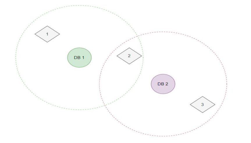
The objective function (8a) of problem B-IFP can be written as:
The objective function (9a) of problem R-BFP can be written as:
The objective function (13a) of problem R-MILP can be written as:
Appendix E Size of Formulations
Number of constraints Number of binary variables Number of general integer variables 0
Appendix F Pseudo-code of Outer Approximation Branch-and-Cut Algorithm OA-B&C
-
•
If the objective value corresponding to is not better than that of the incumbent, the node is pruned.
-
•
If the objective value corresponding to is better than that of the incumbent, then:
-
–
If is fractional, apply user callback:
-
*
If violates any constraint in :
-
·
Move violated constraints to and discard .
-
·
Update sets of user cuts and active constraints for each open node
-
·
-
*
If no valid inequality in is violated by , then branching constraints are entered to cut off and the next open node is processed.
-
*
-
–
If is integer-valued, check for possible violation of lazy constraints:
-
*
If violates any constraint in :
-
·
Move violated lazy constraints to and discard .
-
·
Update sets of lazy and active constraints for each open node :
-
·
-
*
If does not violate any constraint in , becomes the incumbent and node is pruned.
-
*
-
–
Appendix G Outer Approximation Algorithm with Lazy Constraints
The outer approximation algorithm OA is designed as follows. At the root node (), we have:
At any node , the reduced-size relaxation (outer approximation) problem is solved:
Two possibilities arise depending on the optimal solution of the continuous relaxation of :
-
(1)
If is fractional, we introduce branching linear inequalities to cut off the fractional nodal optimal solution and we continue the branch-and-bound process.
-
(2)
If is an integer-valued solution with better objective value than the one of the incumbent, we check for possible violation of the current lazy constraints:
-
•
If some constraints in are violated by , they are inserted in and is discarded. The lazy and active constraint sets of each open node are updated as follows:
-
•
If no lazy constraint is violated, becomes the incumbent solution and the node is pruned.
-
•
The above process terminates when all nodes are pruned. The verification of the possible violation of the lazy constraints is carried out within a callback function, which is not performed at each node of the tree, but only when a better integer-valued feasible solution is found.
Appendix H Pseudo-Code of Simulator
We leverage the simulator to generate and compare the average response times obtained with our model R-MILP, an alternative formulation BM, and two constructive greedy heuristics H-DB and H-OTR.
To ensure that the steady state condition holds, we follow the procedure adopted in two recent EMS studies [14, 55] and process first a buffer of overdose requests prior to the period of interest. Experiments show that a buffer of at least five hours of OTR requests produces results that are independent of buffer duration. For each test, we run the simulation 100 times and we record the mean as well as the 5th and 95th percentiles of the response times. As in [33] for the stochastic UAV mission planning with uncertain service times, we sample the service time from a gamma distribution with shape parameter equal to 4 and mean equal to the expected value of .
Algorithm 2 present the pseudo-code of the simulator. We use to denote the current time, to denote the drone flight time from its base to OTR or from OTR to its base, and to denote the combined on-scene service time and time to clean and recharge drones.
Appendix I Data Summary
| Pairs of Sets | Training Sets | - Training | Testing Sets | - Testing |
| (2018Q2, 2018Q3) | 2018Q2 | 173 | 2018Q3 | 131 |
| (2018Q3, 2018Q4) | 2018Q3 | 131 | 2018Q4 | 120 |
| (2018Q4, 2019Q1) | 2018Q4 | 120 | 2019Q1 | 138 |
| (2019Q1, 2019Q2) | 2019Q1 | 138 | 2019Q2 | 171 |
Appendix J Confidence Interval for Response Times of R-MILP
| Training Set | Response Time (min.) for R-MILP | ||
| 5th Percentile | Mean | 95th Percentile | |
| 2018Q2 | 0.80 | 1.49 | 2.19 |
| 2018Q3 | 0.67 | 1.58 | 2.60 |
| 2018Q4 | 0.50 | 1.54 | 2.49 |
| 2019Q1 | 0.45 | 1.50 | 2.50 |
| Quarter Average | 0.61 | 1.53 | 2.45 |
| Training/Testing Data | Testing Quarter Response Time (min.) R-MILP | ||
| 5th Percentile | Mean | 95th Percentile | |
| 2018Q2 / 2018Q3 | 0.82 | 1.72 | 2.79 |
| 2018Q3 / 2018Q4 | 0.54 | 1.57 | 2.55 |
| 2018Q4 / 2019Q1 | 0.74 | 1.80 | 2.83 |
| 2019Q1 / 2019Q2 | 0.57 | 1.48 | 2.38 |
| Quarter Average | 0.67 | 1.64 | 2.64 |
Appendix K Pseudo-codes of Constructive Greedy Heuristics Approaches
Appendix L Comparison with Constructive Greedy Heuristics
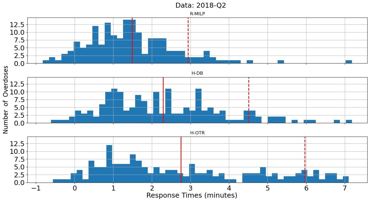
Appendix M Data for QALY and Cost Analysis
| T-QALY | |||
| 11.4 years | 0.85 | 3% | 8.47 years |
| Price per | Annual | Number of | Discount | Total Discounted |
| Drone | Maintenance Cost | Drones | Rate | Cost in 4 Years. |
| $15,000 | $3,000 | 11 | 3% | $287,664 |
Appendix N Computational Efficiency Study
| Instance | Solution Time (sec.) | ||||
| REFO | OA | OA-B&C | R-OA-B&C | ||
| 50 | 1 | 7 | 3 | 3 | 2 |
| 2 | 25 | 3 | 3 | 2 | |
| 3 | 17 | 2 | 2 | 2 | |
| 4 | 17 | 3 | 3 | 2 | |
| 5 | 6 | 3 | 2 | 2 | |
| Average | 14 | 3 | 3 | 2 | |
| 100 | 1 | 3600 | 12 | 11 | 8 |
| 2 | 3600 | 13 | 12 | 9 | |
| 3 | 3600 | 11 | 10 | 8 | |
| 4 | 3600 | 12 | 12 | 9 | |
| 5 | 3600 | 12 | 12 | 9 | |
| Average | 3600 | 12 | 11 | 9 | |
| 150 | 1 | 3600 | 46 | 60 | 34 |
| 2 | 3600 | 47 | 33 | 24 | |
| 3 | 3600 | 37 | 29 | 25 | |
| 4 | 3600 | 41 | 43 | 26 | |
| 5 | 3600 | 39 | 32 | 26 | |
| Average | 3600 | 42 | 39 | 27 | |
| 200 | 1 | 3600 | 170 | 151 | 99 |
| 2 | 3600 | 109 | 105 | 67 | |
| 3 | 3600 | 161 | 122 | 96 | |
| 4 | 3600 | 138 | 170 | 112 | |
| 5 | 3600 | 221 | 169 | 129 | |
| Average | 3600 | 160 | 143 | 101 | |
| 250 | 1 | 3600 | 706 | 358 | 250 |
| 2 | 3600 | 517 | 302 | 200 | |
| 3 | 3600 | 408 | 227 | 232 | |
| 4 | 3600 | 431 | 440 | 265 | |
| 5 | 3600 | 233 | 218 | 237 | |
| Average | 3600 | 459 | 309 | 237 | |
| 300 | 1 | 3600 | 831 | 252 | 406 |
| 2 | 3600 | 608 | 374 | 290 | |
| 3 | 3600 | 935 | 706 | 428 | |
| 4 | 3600 | 656 | 813 | 456 | |
| 5 | 3600 | 288 | 446 | 146 | |
| Average | 3600 | 664 | 518 | 345 | |
| 350 | 1 | 3600 | 595 | 699 | 475 |
| 2 | 3600 | 1160 | 540 | 490 | |
| 3 | 3600 | 3172 | 893 | 497 | |
| 4 | 3600 | 710 | 620 | 429 | |
| 5 | 3600 | 1872 | 337 | 492 | |
| Average | 3600 | 1502 | 618 | 477 | |
| 400 | 1 | 3600 | 1515 | 778 | 545 |
| 2 | 3600 | 1442 | 560 | 803 | |
| 3 | 3600 | 2824 | 1249 | 532 | |
| 4 | 3600 | 596 | 1295 | 365 | |
| 5 | 3600 | 847 | 471 | 655 | |
| Average | 3600 | 1445 | 871 | 580 | |
| 450 | 1 | 3600 | 965 | 669 | 1901 |
| 2 | 3600 | 2155 | 934 | 775 | |
| 3 | 3600 | 3600 | 1815 | 601 | |
| 4 | 3600 | 810 | 833 | 508 | |
| 5 | 3600 | 1966 | 1033 | 2265 | |
| Average | 3600 | 1899 | 1057 | 1210 | |
| 500 | 1 | 3600 | 3600 | 2943 | 1059 |
| 2 | 3600 | 3600 | 1814 | 1245 | |
| 3 | 3600 | 3600 | 3600 | 975 | |
| 4 | 3600 | 2865 | 1208 | 2359 | |
| 5 | 3600 | 1728 | 1872 | 637 | |
| Average | 3600 | 3079 | 2287 | 1255 | |
| Solution Time (seconds) | REFO | OA | OA-B&C | R-OA-B&C |
| 600 | 10% | 54% | 64% | 78% |
| 1200 | 10% | 74% | 84% | 92% |
| 1800 | 10% | 80% | 90% | 94% |
| 2400 | 10% | 86% | 96% | 100% |
| 3000 | 10% | 90% | 98% | 100% |
| 3600 | 10% | 92% | 98% | 100% |