spacing=nonfrench
DP-Forward: Fine-tuning and Inference on Language Models with Differential Privacy in Forward Pass
Abstract.
Differentially private stochastic gradient descent (DP-SGD) adds noise to gradients in back-propagation, safeguarding training data from privacy leakage, particularly membership inference. It fails to cover (inference-time) threats like embedding inversion and sensitive attribute inference. It is also costly in storage and computation when used to fine-tune large pre-trained language models (LMs).
We propose DP-Forward, which directly perturbs embedding matrices in the forward pass of LMs. It satisfies stringent local DP requirements for training and inference data. To instantiate it using the smallest matrix-valued noise, we devise an analytic matrix Gaussian mechanism (aMGM) by drawing possibly non-i.i.d. noise from a matrix Gaussian distribution. We then investigate perturbing outputs from different hidden (sub-)layers of LMs with aMGM noises. Its utility on three typical tasks almost hits the non-private baseline and outperforms DP-SGD by up to pp at a moderate privacy level. It saves time and memory costs compared to DP-SGD with the latest high-speed library. It also reduces the average success rates of embedding inversion and sensitive attribute inference by up to pp and pp, respectively, whereas DP-SGD fails.
1. Introduction
The deep learning architecture of transformer (Vaswani et al., 2017) is now gaining popularity in computer vision and has been widely utilized in natural language processing (NLP). Transformer-based language models (LMs), such as BERT (Devlin et al., 2019) and GPT (Radford et al., 2018, 2019), have remarkably achieved state-of-the-art performance in almost every NLP task. They are first pre-trained on massive (public) self-labeled corpora and then fine-tuned for various tasks using much smaller, potentially private corpora. It avoids training from scratch and the possible shortage of task-specific corpora while earning versatility.
Training data contributing to the improved utility of fine-tuned LMs can be sensitive. LMs can (unintentionally) memorize them (Carlini et al., 2019) and become vulnerable to membership inference attacks (MIAs) (Shokri et al., 2017) that identify whether an example is in the training set. Worse still, verbatim training text (e.g., SSNs) can be extracted via only black-box access to GPT-2 (Carlini et al., 2021). It is also possible to recover personal health information (e.g., patient-condition pairs) from BERT trained over a clinical corpus (Lehman et al., 2021) based on the extraction attack (Carlini et al., 2021).
Differential privacy (DP) (Dwork et al., 2006) has emerged as the de facto privacy standard for protecting individual privacy. To thwart MIAs on individuals’ training data, DP stochastic gradient descent (DP-SGD) (Abadi et al., 2016) can be used. It clips the gradients of each example in a batch and adds random Gaussian noise to the aggregated gradient. It is more general than earlier attempts (Chaudhuri and Monteleoni, 2008; Chaudhuri et al., 2011) that focus on convex problems and has been implemented in modern ML frameworks, such as PyTorch and TensorFlow. One can apply it to fine-tune LM-based NLP pipelines while ensuring example-level privacy, assuming each individual contributes an example, typically a sequence-label pair.
Unfortunately, DP-SGD often uses a trusted party to curate users’ sensitive training data. Although it can be done distributively (Bonawitz et al., 2017; McMahan et al., 2018) via secure aggregation (Chase and Chow, 2009) with extra costs and trust assumptions, it offers central DP (CDP) at its core.111Distributed DP-SGD adds local noise too small to achieve LDP. But it is protected by secret sharing. When all shares are aggregated, they cancel out each other, assuming an honest majority. It thus faces a “synchronization” issue begging for identification and recovery mechanisms with computation and communication overheads (Bonawitz et al., 2017). Instantiating per-example gradients as large as entire pipelines (e.g., M parameters for BERT-Base) is obliviously costly. Moreover, maintaining the utility of pipelines trained by the noisy aggregated one is tricky due to the dimensional “curse.” A recent study (Yu et al., 2021, Table ) shows that the average accuracy in fine-tuning LMs for four NLP tasks at moderate privacy is (vs. without DP). Finally, the inference-time embeddings are not perturbed by the noise added during training, leaving inference queries vulnerable to various recovery attacks (Song and Raghunathan, 2020; Pan et al., 2020), ranging from sensitive attributes (e.g., authorship) to raw text.
1.1. Natural Privacy via Perturbing Embeddings
We propose DP-Forward, a radically different approach that perturbs forward-pass signals: Users can locally inject noise into the embeddings of (labeled) sequences before sharing them for training, in contrast to perturbing gradients in back-propagation (possibly by an untrusted party). It is meant for provable local DP (LDP) guarantees, thus protecting against stronger adversaries than DP-SGD.
Our approach also naturally fits the federated learning (FL) setting that does not gather users’ data but with substantial differences – FL typically shares noiseless local model updates. Note that any subsequent computation (e.g., gradient computation) on noisy embeddings incurs no extra privacy loss due to the free post-processing of LDP. One might force DP-SGD to offer LDP by adding “enough” noise to the orders-of-magnitude larger per-example gradient from a user, but it may yield unusable models at a similar privacy level.
DP-Forward also extends its applicability to inference via adding noise to users’ test-sequence embeddings, ensuring LDP as in training. As a “side” benefit, it can effectively mitigate emerging embedding-based privacy risks (Pan et al., 2020; Song and Raghunathan, 2020) beyond MIAs.
It is evident that the design goals of DP-Forward naturally align in tandem with our overarching objectives: LDP (vs. CDP), more direct protection of raw data (vs. gradients) against new threats (Pan et al., 2020; Song and Raghunathan, 2020), and can be as efficient as regular non-private training (allowing batch processing of noisy embeddings). The foundation supporting these desiderata, unfortunately, was unavailable. A dedicated mechanism to perturb the forward-pass signals is indispensable.
Specifically, we need to derive noises for embeddings of training/inference text sequences obtained through the forward pass of LM-based pipelines as a real- and matrix-valued function. One might adopt the classical Gaussian mechanism (GM) (Dwork and Roth, 2014) to add i.i.d. noise drawn from a univariate Gaussian distribution. Yet, GM calibrates its noise variance based solely on a sufficient condition for DP, and its variance formula is not applicable to a low privacy regime (Balle and Wang, 2018). Another candidate is the matrix-variate Gaussian (MVG) mechanism (Chanyaswad et al., 2018), tailored for matrix-valued data: It exploits possibly non-i.i.d. noise from a matrix Gaussian distribution to perturb more important rows/columns less. Although it may show better utility over GM (Chanyaswad et al., 2018), it is still sub-optimal due to the sufficient condition.
To optimize MVG, we propose an analytic matrix Gaussian mechanism (aMGM) by integrating a necessary and sufficient condition from the analytic GM (aGM) (Balle and Wang, 2018) for non-i.i.d. noise calibration. Our challenge lies in manipulating the two covariance matrices instead of a single variance. We deduce a constraint only on the two smallest singular values (Section 4.2), indicating that i.i.d. noise (as in aGM) may already be optimal for general applications like DP-Forward.222 With extra assumptions, dedicated allocation of other singular values by optimizing/maximizing utility functions specific to applications could help.
A transformer-based pipeline contains an input embedding layer, encoders, and task layers. All these layers prominently manipulate embeddings of text inputs in training and subsequent inference. We investigate adding aMGM noise to embeddings output by any hidden (sub-)layer before task layers (Figure 1). To ensure sequence-level LDP, we need to estimate the -sensitivity (Dwork and Roth, 2014) of “pre-noise” functions for any two sequences. It is non-trivial since the functions can include different (sub-)layers that may not even be Lipschitz (Kim et al., 2021). Our strategy is to normalize the function outputs to have a fixed Frobenius (or ) norm, similar to gradient clipping (Abadi et al., 2016). It works especially well for deeper sub-layers, achieving comparable task accuracy to the non-private baseline (Section 5). For the first few (sub-)layers, we also make two specializations in relaxing LDP to the token level, elaborated in Appendix A.2, to improve accuracy.

1.2. Our Contributions
Motivated by prevailing privacy concerns in LM fine-tuning and inference and inherent shortcomings of DP-SGD, we initiate a formal study of an intuitive but rarely studied approach and explore its integration with a transformer-based NLP pipeline. Specifically:
1) We propose DP-Forward fine-tuning, which perturbs the forward-pass embeddings of every user’s (labeled) sequence. It offers more direct protection than DP-SGD perturbing aggregated gradients. Its provable guarantee (Theorem 3) is a new sequence-level LDP notion (SeqLDP, Definition 2), with the more stringent -LDP guarantee to hold w.r.t. only sequences. Moreover, DP-Forward can naturally extend to inference, ensuring the standard LDP (Theorem 5) for test sequences without labels, whereas DP-SGD cannot.
2) To instantiate an optimal output perturbation mechanism for DP-Forward, we propose aMGM, owning independent interests for any matrix-valued function. By exploiting a necessary and sufficient DP condition from aGM (Balle and Wang, 2018), it can draw possibly non-i.i.d. noise from a matrix Gaussian distribution like MVG (Chanyaswad et al., 2018) while producing orders-of-magnitude smaller noise for high-dimensional data (Section 5.3).
3) We conduct experiments333Our code is available at https://github.com/xiangyue9607/DP-Forward. on three typical NLP tasks in Section 5, showing how crucial hyperparameters (e.g., the sequence length) impact task accuracy. To fairly compare with DP-SGD on privacy-vs.-utility: i) We perturb labels by the randomized response (Warner, 1965) such that DP-Forward fine-tuning offers the standard LDP for sequence-label pairs (Theorem 4). ii) We “translate” DP-Forward with standard LDP to (example-level) CDP (as offered by DP-SGD) via shuffling (Erlingsson et al., 2019). Our accuracy gain (for deep-layer DP-Forward instantiations) is up to percentage points (pp), compared to DP-SGD or its recent improvements (Yu et al., 2021, 2022) (reviewed in Section 7.3), at a similar privacy level. Efficiency-wise, DP-SGD incurs time and GPU-memory costs even with the latest Opacus library (Yousefpour et al., 2021).
4) We evaluate three classes of privacy threats. Like DP-SGD, DP-Forward (including the two token-level designs in Appendix A.3) can effectively defend against sequence-level MIAs, but only DP-Forward can thwart the two threats on (inference-time) embeddings. Specifically, Section 6 shows that DP-SGD totally fails in two embedding inversion attacks, while DP-Forward remarkably reduces their success rates by up to pp. For a neural-network-based attribute inference attack, DP-SGD reduces its success rates by only pp on average, while DP-Forward achieves pp reduction, making the attack predict like assigning all labels to the majority class.
In short, DP-Forward is a better alternative to DP-SGD in training (and testing) deep-learning models, e.g., gigantic LM-based ones.
2. Preliminaries and Notations
2.1. Transformer Encoders in BERT
Modern transformer-based LMs, including BERT (Devlin et al., 2019) and GPT (Radford et al., 2018), are first pre-trained on enormous unannotated (public) corpora to learn contextualized text representations. Later, they can be fine-tuned for various downstream NLP tasks (e.g., sentiment analysis, question answering) using much smaller, task-specific datasets.
We consider BERT (Figure 1), which comprises a stack of identical layers (i.e., bidirectional transformer encoders (Vaswani et al., 2017)). Each layer has two sub-layers: the dot-product multi-head attention (MHA) (Vaswani et al., 2017) with heads and a feed-forward network (FFN). Each sub-layer has an extra residual connection, followed by layer normalization (Ba et al., 2016).
Let be an input sequence of tokens (e.g., characters, words, sub-words, q-grams), where is from a vocabulary . The input embedding layer first maps each to its representation in , which is the sum of the token, segment, and position embeddings. We re-use to represent the hidden embedding matrix in . For each of attentions in the MHA layer, we derive the query, key, and value matrices ( divides ) by multiplying with head-specific weights . Its output is
The input to is an matrix of pairwise dot products. Finally, MHA concatenates (denoted by ) all the head outputs into a matrix in , right multiplied by a projection matrix :
FFN is composed of two linear mappings with a ReLU activation in between. It separately and identically operates on each ,
where , , , and are trainable matrix/vector-valued parameters. Its output on is . The residual connection for sub-layers is . The layer normalization normalizes all entries to have zero mean and unit variance using an extra scale-then-shift step.
At the output of the final encoder, the hidden embedding matrix is reduced to a sequence feature in . Standard reduction methods include mean pooling (Reimers and Gurevych, 2019) (computing ) or taking the last embedding of a special token [CLS] for classification (Devlin et al., 2019).
The pre-training of BERT is based on two self-supervised tasks: masked language model (MLM) and next sentence prediction (Devlin et al., 2019). We adopt MLM: It randomly masks out some tokens, indexed by , in an input sequence . The objective is to predict those masked tokens using their context by minimizing the cross-entropy loss
| (1) |
where denotes all the parameters of BERT transformer encoders.
2.2. (Local) Differential Privacy
DP (Dwork et al., 2006) is a rigorous, quantifiable privacy notion. It has two popular models, central and local. In central DP, a trusted data curator accesses the set of all individuals’ raw data and processes by a randomized mechanism with some random noise. Formally:
Definition 0 (Central DP).
For privacy parameters and , fulfills -DP if, for all neighboring datasets and (denoted by ) and any subset of the outputs of ,
We call it -DP or pure DP when .
The neighboring notion is application-dependent (to be discussed in Section 3.1). Typically, it involves the “replace-one” relation: can be obtained from by replacing a single individual’s data point (e.g., a sequence-label pair). CDP offers plausible deniability to any individual in a dataset. In contrast, local DP (LDP) (Kasiviswanathan et al., 2008) removes the trusted curator, allowing individuals to locally perturb their data using before being sent to an untrusted aggregator for analytics.
Definition 0 (Local DP).
For , is -LDP if, for any two inputs and any possible output subset of ,
Similarly, we call it -LDP when .
Privacy Loss Random Variable (PLRV)
For a specific pair of inputs , the privacy loss (or the “actual value”) (Balle and Wang, 2018) incurred by observing an output is the log-ratio of two probabilities:
When varies according to , we get the PLRV . A helpful way to work with DP is to analyze tail bounds on PLRVs (Dwork and Roth, 2014), which we utilize to build our proposed mechanism in Section 4.2.
DP has two desirable properties: free post-processing and composability. The former means that further computations on the outputs of an -DP mechanism incur no extra privacy loss. The latter allows us to build more complicated mechanisms atop simpler ones: sequentially (and adaptively) running an -DP mechanism for times on the same input is at least -DP. The two properties also hold for LDP when considering a dataset has only one row.
An output perturbation mechanism for a matrix-valued function is given by computing on the inputs and then adding random noise drawn from a random variable to its outputs.
Gaussian Mechanism (GM). For -DP, a typical instance of is the classical GM (Dwork and Roth, 2014), which adds noise with each entry i.i.d. drawn from a univariate Gaussian distribution . The variance with the -sensitivity:
where denotes the matrix Frobenius norm (Horn and Johnson, 2012).
Table 1 summarizes the acronyms throughout this work.
| NLP | Natural Language Processing |
|---|---|
| LM | Language Model |
| BERT | Bidirectional Encoder Representations from Transformers |
| MLM | Masked Language Modeling |
| MHA | Multi-Head Attention |
| FFN | Feed-Forward Network |
| MIA | Membership Inference Attack |
| DP-SGD | Differentially Private Stochastic Gradient Descent |
| PLRV | Privacy Loss Random Variable |
| (C)DP | (Central) Differential Privacy |
| LDP | Local Differential Privacy |
| Seq(L)DP∗ | Sequence (Local) Differential Privacy |
| GM | Gaussian Mechanism |
| RR | Randomized Response |
| MVG | Matrix-Variate Gaussian (Mechanism) |
| aGM | Analytic Gaussian Mechanism |
| aMGM∗ | Analytic Matrix Gaussian Mechanism |
3. DP-Forward
We study BERT-based pipelines as an example due to their superior performance in classification tasks. DP-Forward can be readily applied to other (transformer-based) NLP or computer vision models that involve matrix-valued computation during the forward pass.
Suppose each user holds a sequence-label pair or only for fine-tuning or testing a pipeline at an untrusted service provider. Sharing redacted (with common PII removed) or its feature, a non-human-readable real-valued embedding matrix, is leaky (Sweeney, 2015; Song and Raghunathan, 2020; Pan et al., 2020).
For DP-Forward training, users perturb their embedding matrices locally to ensure (new notions of) LDP before being shared, and they should also perturb the corresponding labels if deemed sensitive (Section 3.4). We explore different options for splitting pipelines into pre-noise functions and post-noise processing in Section 3.2: Users can access to derive embedding matrices, perturbed by an output perturbation mechanism (e.g., GM); the service provider runs on noisy (labeled) embeddings for fine-tuning (Section 3.3) or pre-training (Section 3.6). The challenge lies in analyzing for different pipeline parts, which we address by normalizing .
DP-Forward can be naturally used to protect inference sequences (Section 3.5), unlike DP-SGD. It exploits the free post-processing (i.e., inference works on noisy embeddings), incurring minimal changes to pipelines with the extra “plug-and-play” noise layer.
3.1. Notions of Sequence (Local) DP
Embeddings encode semantic information of input sequences , each of which has tokens (Section 2.1). Fine-tuning (or subsequent inference of) NLP pipelines essentially processes . DP-Forward fine-tuning protects every by an output perturbation mechanism over , in contrast to DP-SGD, which perturbs aggregates of gradients over and label . Simply put, our -LDP holds for while DP-SGD provides CDP for .
Sequence-only protection is meaningful since sequences often convey (implicit) sensitive information (e.g., authorship), whereas labels (e.g., a single bit denoting positive/negative) can be public. We defer to Section 3.4 for achieving “full” LDP over . To bridge the gap between theoretical guarantees of DP-SGD and DP-Forward, we first define sequence DP444One could generalize it to “feature” (or “input”) DP, as DP-Forward also allows other types of features beyond embeddings (and its essence is input-only privacy). To keep our focus on NLP, we use “sequence” here. (PixelDP (Lécuyer et al., 2019) treats pixels as image features.) (SeqDP) in the central setting.
Definition 0 (SeqDP).
For , is -SeqDP, if that only differ in a sequence at some index : and , and any possible output subset ,
3.1.1. Label DP
The recently proposed notion of label DP (Ghazi et al., 2021; Esmaeili et al., 2021) is originally studied in PAC learning (Chaudhuri and Hsu, 2011). It only protects labels (not the corresponding inputs/images): -DP is only w.r.t. labels.
Our SeqDP is “more secure” than or at least “complements” label DP, which has an inherent flaw (Busa-Fekete et al., 2021): As labels typically rely on their sequences (but not vice versa), it is very likely to recover the true labels from the raw sequences, even if the labels are protected (by any label-DP mechanism). The follow-up (Wu et al., 2023) shows the impossibility of label protection under label DP even with arbitrarily small when models generalize. Moreover, labels can be absent (e.g., inference or self-supervised learning), for which SeqDP upgrades to the standard -DP, whereas label DP is simply inapplicable.
3.1.2. Sequence Local DP (SeqLDP)
We further define SeqLDP, the local counterpart of sequence DP. Note that the above discussion of label DP in relation to SeqDP also carries over to SeqLDP.
Definition 0 (SeqLDP).
For , satisfies -SeqLDP, if with the same , and any possible output subset ,
In theory, SeqLDP remains a strong notion (like the standard LDP). It is meant to be information-theoretic protection on sequence and bounds the indistinguishability of any (differing by up to tokens), and hence governing the “usefulness” of noisy embeddings.
3.1.3. Sequence-Level SeqLDP vs. Token-Level SeqLDP
In practice, as a strong notion balancing seemingly conflicting requirements (ideal theoretical guarantees and empirical utility), attaining a meaningful range of for SeqLDP is a struggle. Adding Gaussian noise to the outputs of for -SeqLDP requires bounding the -sensitivity . Our approach is to normalize the outputs (with extra benefits elaborated in Section 3.2), similar to clipping gradients in DP-SGD. It generally works better when has more layers (at the same meaningful range of ) since fewer (trainable) parameters/layers of are “affected” by the noisy outputs.
Unfortunately, when includes the first few layer(s), e.g., only the input embedding layer is available to the users (say, for saving user-side storage and computation overheads), it leads to poor utility. As a comprehensive study, we resort to row-wise normalization with the (composition of) Lipschitz constants (Kim et al., 2021) to maintain utility for those cases.555One might also resort to the weaker random DP (Hall et al., 2013) – -DP holds on all but a small -proportion of “unlikely” for an extra parameter . It is useful when the global sensitivity is hard to compute. Exploring it is left as future work. In contrast to the general normalization, it aims for weaker SeqLDP at the token level (cf. event-level vs. user-level LDP (Zhou et al., 2022)), a finer granularity in the “protection hierarchy,” protecting any neighboring sequences (vs. datasets) differing in any single token (vs. sequence). Details are deferred to Appendix A.
3.2. Our Approach for Sequence LDP
DP-Forward in our paper (except Appendix A) applies the general normalization approach to any for sequence-level (Seq)LDP.
Let be an arbitrarily deep forward pass, ranging from the first (input embedding) layer itself to all but the last (task) layer in a BERT-based pipeline (Figure 1). Correspondingly, let be the remaining layers, ranging from the last task layers themselves to all but the first (input embedding) layer. Every sequence becomes an embedding matrix at the output of layers in encoders or before task layers (Section 2.1). To offer -SeqLDP, we adopt a suitable output perturbation mechanism , such as GM, considering that a dataset has only one labeled sequence.
Since can work on the output of any hidden layer, estimating is non-trivial. Specifically, itself, let alone more layers included, is not Lipschitz continuous, meaning its outputs can change arbitrarily for even slight input variation (Kim et al., 2021). To address this, our approach is to normalize or clip the function outputs:
as in DP-SGD (Abadi et al., 2016), where is a tunable parameter. We then have . Such normalization makes task utility less “sensitive” to the choice of since signal and noise increase proportionally with , whereas the signal may be unchanged when is not clipped. It also has many other benefits, such as stabilizing training, avoiding overfitting, and accelerating convergence (Aboagye et al., 2022). Hence, we resort to normalization in our experiments. One can then calibrate Gaussian noise and derive for the post-noise layers .
Note that we remove the residual connection when adding noise to the output of the first MHA layer to avoid reaccessing (dashed arrow, Figure 1) to maintain free post-processing. This may lead to instability (e.g., gradient vanishing) (Yu et al., 2021), but it can be mitigated by pre-training new BERT without such a residual connection to keep consistent with later fine-tuning/inference.
DP-Forward using GM suffers from the “curse of dimensionality” when is large (e.g., for BERT-Base). To alleviate the curse, we can append two linear maps, with , such that and respectively have and . Both maps are randomly initialized and updated like other weights using gradients. The raw embedding matrix is first right multiplied by , leading to or , before being normalized. Our privacy guarantee will not be affected since remains the same. We then use to restore the dimensionality to be compatible with the raw pipeline; incurs no extra privacy loss due to the free post-processing. Nevertheless, it needs dedicated efforts to modify the pipeline; dimension-reduced embedding matrices may also lose useful information, degrading task utility. We thus make and optional (see Section 5.2).
3.3. DP-Forward Fine-tuning
Suppose we use a raw, public BERT checkpoint666Using noisy BERT for fine-tuning (and subsequent inference) is deferred to Section 3.6. for fine-tuning. In the forward pass of the -th () step, it offers the latest to a batch of users, mimicking the regular mini-batch SGD. is from the raw checkpoint. Users are randomly chosen (without replacement), and their number is a fixed parameter. Users in the batch individually compute their noisy embeddings to ensure SeqLDP (Theorem 3). They then send them with unperturbed labels to the service provider, who runs over to compute the batch loss; any post-processing of embeddings under SeqLDP incurs no extra privacy degradation on . here includes the rest raw BERT part and randomly initialized task layers.
During the back-propagation, the service provider can update to via the gradient (derived from the loss and noisy embeddings) of the post-noise layers. To avoid accessing users’ raw , it needs to freeze the pre-noise layers as . Parameter freezing is compatible with the more recent zero-shot or in-context learning paradigm (Min et al., 2022). It is useful when models are gigantic and full fine-tuning is expensive. However, the more layers are frozen, the worse the utility might be (even in non-private settings).
There are two general ways to update securely: i) We can assume an extra trusted party (as in DP-SGD), but it becomes central DP. ii) Users can first derive the gradients for the layers inside locally on their and then resort to secure aggregation (Bonawitz et al., 2017) for global updates at the service provider. However, it is costly. For better utility, we update in experiments, requiring us to consider privacy degradation across different epochs due to the composability (as detailed below). Dedicated approaches (that balance efficiency, privacy, and utility) are left as future work.
Theorem 3.
Let be the pre-noise function (of BERT-based pipelines) and be GM with . DP-Forward fine-tuning running on normalized/clipped ensures -SeqLDP.
The proof follows that of GM (Dwork and Roth, 2014). The crux is that is given by the output normalization, independent of the inputs.
Privacy Accounting. An epoch refers to an entire transit of the private training corpus. Every is used once per epoch. The number of epochs is a hyperparameter, which is typically small. Repeated applications of GM over the same ask for estimating the overall privacy loss due to the composability (unless freezing for re-using ). The well-known moments accountant (Abadi et al., 2016) (or its generalization to Rényi DP (Mironov, 2017)) only provides a loose upper bound, which is even inapplicable if unbounded moments exist. Gaussian DP (Bu et al., 2019) proposes an accountant based on the central limit theorem. Yet, it leads to significant underestimation by a lower bound. Instead, we resort to a recent numerical accountant (Gopi et al., 2021), which outperforms RDP or GDP by approximating the true overall to arbitrary accuracy. It composes the privacy curve of a mechanism by truncating and discretizing PLRVs with their PDFs convoluted by FFT (Gopi et al., 2021).
3.4. DP-Forward with Shuffling versus DP-SGD
DP-Forward ensures SeqLDP for fine-tuning, while DP-SGD offers central DP (for sequence-label pairs). To facilitate a fair comparison (on privacy-utility tradeoffs), we make two changes. First, we also perturb the labels with a suitable mechanism for the standard LDP, i.e., extending the protection from sequence to sequence-label pairs. Second, we use shuffling (Erlingsson et al., 2019) to “translate” our (label-protected) DP-Forward with LDP to claim (example-level) CDP as DP-SGD.
Discrete Labels Perturbation. For most NLP tasks, e.g., bi-/multi-nary classification in the GLUE benchmark (Wang et al., 2019), the size of label space is often small. A simple yet effective solution for discrete data is randomized response (RR) (Warner, 1965) proposed decades ago! Specifically, RR perturbs a true label to itself with the probability
or to uniformly, where denotes the label space.
When is large, we can use prior to “prune” to smaller (Ghazi et al., 2021). The prior can be publicly available (e.g., auxiliary corpora similar to the users’ data) or progressively refined from a uniform distribution via the multi-stage training (Ghazi et al., 2021). One can then estimate an optimal by maximizing the probability that the output is correct, i.e., . With (prior-aided) RR (Ghazi et al., 2021), we can achieve full LDP.
Theorem 4.
Let be the pre-noise function (of BERT-based pipelines), be GM with , and be (prior-aided) RR with . DP-Forward fine-tuning perturbing and separately by and ensures -LDP.
The proof follows from the basic composition theorem (Dwork and Roth, 2014).
Privacy Amplification by Shuffling. If noisy embedding-label pairs are also shuffled properly, DP-Forward can claim example-level CDP (as in DP-SGD), which “amplifies” LDP guarantees by for a total number of users (without extra noise addition) (Erlingsson et al., 2019). We then show that DP-Forward qualitatively outperforms DP-SGD from the SNR perspective under a similar privacy regime.
Suppose we train for an epoch, and the normalization factor is . For DP-SGD, the batch size is ; the subsampling probability and the number of training steps are respectively and . If each step is -DP, the overall privacy loss is -DP using the strong composition and privacy amplification by subsampling (Abadi et al., 2016).
DP-Forward with shuffling can also be seen as composing subsamplings, each a fraction of size (Steinke, 2022). It is -DP, which is “amplified” from -LDP. For an easier analysis of SNR, we omit of RR since the overall is dominated by composing subsampled Gaussian. So, our Gaussian noise variance is smaller than DP-SGD’s in each step; the SNR of each entry in embeddings vs. the aggregation of gradients can be estimated as for DP-Forward vs. for DP-SGD, where is the gradient dimension and is much larger than , the embedding-matrix size.
3.5. DP-Forward Inference
Given only fine-tuned pipeline parts , users can derive the noisy embedding matrices of their test sequences for inferences at the service provider while ensuring -LDP. Inference using noise aligned to the noisy fine-tuning is also beneficial for task accuracy.
Local inference (as in DP-SGD) without noise forces the service provider to reveal its entire pipeline, losing its intellectual property and incurring more time and storage costs for both and .
Theorem 5.
Let be the fine-tuned pre-noise layers (of BERT-based pipelines) and be GM with . DP-Forward inference running on normalized/clipped ensures -LDP.
The proof is inherited from GM (Dwork and Roth, 2014). Different from DP-Forward fine-tuning, LDP holds for test sequences since the labels are absent.
3.6. DP-Forward Pre-training
Directly using the raw BERT might not “match” DP-Forward fine-tuning/inference, degrading task utility. Pre-training BERT with DP-Forward on publicly available text (e.g., Wikipedia), besides the private user-shared data, can make future operations “adaptive” to noise. It requires us to modify the raw MLM objective in Eq. (1):
where denotes the parameters of “noisy” BERT. This endows the noisy BERT with some “de-noising” ability since the objective is to predict the raw masked tokens from noisy embeddings . It does not really breach privacy due to the free post-processing; LDP is ensured for each sequence, as the pre-training is self-supervised (without labels). Such noisy pre-training can also be outsourced to dedicated GPU clusters, enabling “de-noising BERT as a service.”
De-noising as post-processing is not new, but most prior arts need prior knowledge, e.g., Bayesian prior. aGM formulates it as an unusual estimation problem since a single noisy output is observed for each input, which can then be solved by appropriate estimators, e.g., the Bayesian one (Balle and Wang, 2018). Another attempt (Lécuyer et al., 2019) trains a separate noisy auto-encoder, which learns the identity function stacked before an image classification network, to de-noise the noisy input. It has limited applications for only noisy input embeddings and incurs extra changes when migrating it to an NLP pipeline.
4. Optimizing Matrix Gaussian Noise
To instantiate for of DP-Forward, a natural question is whether the classical GM is optimal. The answer is no. Its privacy analysis applies a sufficient but not necessary condition for -DP while using Gaussian tail approximations, and its variance formula cannot extend to for a single run (e.g., inference) (Dwork and Roth, 2014).
Another candidate is the matrix-variate Gaussian (MVG) mechanism (Chanyaswad et al., 2018), tailored for matrix-valued functions. It exploits possibly non-i.i.d. noise from a matrix Gaussian distribution and outperforms GM in several usage cases (Chanyaswad et al., 2018). Yet, it is not optimal either, with the root cause still being based on a sufficient DP condition (Section 4.1). To improve it, we resort to a necessary and sufficient condition from aGM (Balle and Wang, 2018) for calibrating the matrix Gaussian noise (Section 4.2).
4.1. Matrix-Variate Gaussian (MVG) Mechanism
In contrast to the classical GM, MVG adopts possibly non-i.i.d. noise drawn from the zero-mean matrix Gaussian distribution , where and are the row- and column-wise covariance matrices. Intuitively, it adds less noise to more “important” rows or columns for possible better utility.
Definition 0 (Matrix Gaussian Distribution).
The PDF for an random variable following has the form:
| (2) |
where and are invertible with and , and denotes the matrix determinant (Horn and Johnson, 2012).
The definition is equivalent to the conventional form given by the matrix trace. It generalizes the univariate Gaussian used in GM; becomes i.i.d. when are diagonal and equal-valued. Below recites the main theorem of the MVG mechanism for -DP.
Theorem 2 (The MVG Mechanism with -DP (Chanyaswad et al., 2018)).
Let
be the vectors of (non-increasingly ordered) singular values of and , respectively. The MVG mechanism using noise from the matrix Gaussian distribution satisfies -DP if
where , , with (or ) being the generalized harmonic number of order (of ), being , and .
To illustrate how the MVG mechanism works, we quote an example (Chanyaswad et al., 2018): performing regression using an identity query on a liver disorders dataset (McDermott and Forsyth, 2016) with features and samples (i.e., ). MVG treats ‘ALT’ and a teacher label as the two most indicative features based on some prior, thus added with less noise (Chanyaswad et al., 2018). To report the best empirical results, it tries different precision budget (or noise variance) allocation strategies so that the total budget (Theorem 2) is not overspent. For example, it evenly allocates (a tunable parameter) of the budget to the two important features and the rest to the other four. Compared to GM using i.i.d. Gaussian noise, MVG can improve root mean square error (RMSE) by up to at the same privacy level (Chanyaswad et al., 2018).
Sub-optimality of MVG. Theorem 2 presents an upper bound on the product of -norms of two singular-value vectors and , assuming is bounded for any by a constant . The upper bound monotonically decreases with that depends on and approaches as , making the sums of noise variances large. A similar situation exists in high privacy regimes .
At least two slacks caused the sub-optimality. The first and foremost is due to a sufficient condition for -DP (Dwork and Roth, 2014): , which is also used in the classical GM. With the Laurent-Massart Theorem (Laurent and Massart, 2000), MVG further transforms it to for a subset of all the possible outputs. The second lies in a loose matrix-trace-based privacy analysis; a follow-up (Yang et al., 2023) derives a tighter bound from Definition 1 and a matrix-norm inequality.
4.2. Analytic Matrix Gaussian Mechanism
To enhance MVG while still adding possibly non-i.i.d. noise , we put forth the analytic matrix Gaussian mechanism (aMGM) by exploiting a necessary and sufficient condition for -DP, which is formulated using two PLRVs by the analytic GM (aGM) (Balle and Wang, 2018). It is non-trivial777A recent pre-print (Yang et al., 2021) also studied using matrix Gaussian distribution. The proof of (Yang et al., 2021, Lemma ), pivotal for our Theorem 6, is problematic. We prove it in Appendix C. since we now need to work with two covariance matrices and instead of a single variance in aGM.
Theorem 3 ((Balle and Wang, 2018)).
A mechanism is -DP iff, ,
| (3) |
It directly implies the sufficient condition due to . We next show that or of aMGM is also Gaussian, a similar result has been proven in aGM (Balle and Wang, 2018, Lemma 3).
Lemma 0.
The PLRVs of our aMGM follow a distribution with , where .
With Lemma 4, we can then specialize the left-hand side of Eq. (3). Particularly, we use the Gaussian cumulative density function (CDF)
to explicitly express the two probabilities (see Lemma 5) instead of approximating them by the tail bounds of a Gaussian distribution.
Lemma 0.
For any , let with . The following holds for any :
We can further re-write the left-hand side of Eq. (3) as :
| (4) |
a function of and ; it is defined w.r.t. and for aGM (Balle and Wang, 2018). To satisfy Theorem 3, we require . Since is monotonically increasing (Balle and Wang, 2018, Lemma 7), we first find the upper bound of as the “solution” to and then determine (hence ) based on and with .
4.2.1. Computing the upper bound
One could derive an analytic expression for using the tail bounds of , which is sub-optimal due to the slack in the tail bounds. Instead, we adapt a “numerical solver,” as detailed in Alg. 1, for since can also be represented by , where is the standard error function.888Its efficient implementation to extremely high accuracy is supported in most statistical and numerical software packages, e.g., Python math library.
For the first term of Eq. (4), its input changes sign at , while the other term’s input is always negative. Therefore, we only consider under two cases and for a variable .
When , in line . If (or ), we can use to re-write as (line 3). For , we can use to re-write as (line 7). In either case, given the “oracle” computing via , we derive or using Newton’s method, recover , and return .
4.2.2. Determining the covariance matrices and
With Lemma 5, and let be the singular value; we have
| (5) |
Since and with , we transform the right-hand side of Eq. (5) to
where the inequality follows from Theorem 2, i.e., , and the last equality is directly from Lemma 4.
Given , it suffices to let with . Recall that is the upper bound on , we now reach the main theorem.
Theorem 6.
Our aMGM satisfies -DP, iff
where as in Alg. 1, is the -sensitivity, and are respectively the smallest singular values of and .
Theorem 6 only constrains the lower bound on the product of and , the two smallest singular values; it offers infinite choices for all the others with the design space for even larger than that of MVG (Theorem 2). More importantly, the lower bound is independent of , which can lead to orders-of-magnitude variance reduction than MVG, confirmed by our experiments in Section 5. For , we can still derive a valid from .
To determine , another implicit constraint is to keep smaller noise for better utility. Let us first consider . Since it is positive definite, we can also decompose it into ; we then have , where specifies the row-wise noise magnitudes. Assuming that the smallest overall noise will yield the best utility, we let all the singular values be the smallest: . As can be any unitary matrix, we simply use the standard basis, resulting in for an identity matrix and hence the final . Similarly, we can pick with , where is a identity matrix.
4.2.3. Drawing the noise
With and , the last step is to draw . Pragmatically, we adopt the affine transformation below.
Lemma 0 ((Chanyaswad et al., 2018)).
Let be a random variable with each entry i.i.d. drawn from the standard normal distribution. The transformed follows .
Hence, we can first sample i.i.d. values from to form , then employ the transformation such that
| (6) |
Discussion.
When instantiating DP-Forward using aMGM, we set and such that the row- and column-wise noises are the smallest, and our pilot experiments show this yields optimal task utility; aMGM actually “degenerates” to aGM with i.i.d. noise. Nevertheless, aMGM also allows non-i.i.d. noise like MVG: By tuning the corresponding singular values larger, we can add more noise to the rows/columns that negatively impact the utility. It might be helpful when (e.g., linear regression on a small liver dataset (Chanyaswad et al., 2018)) is simple or does not “mix up” noisy rows/columns. In contrast to our empirical approach (like MVG), one could theoretically formulate the allocation of singular values as optimization problems that maximize different utility functions tailored to applications. It might outperform our uniform treatment but takes more dedicated efforts, which we leave as future work.
5. Experiments
5.1. Experimental Setup


We use three typical datasets/tasks that are widely used in NLP/DP literature (Yu et al., 2021; Li et al., 2022b; Yu et al., 2022; Yue et al., 2021) and GLUE benchmark (Wang et al., 2019): i) Stanford sentiment treebank (SST-2), ii) Internet movie database (IMDb) (Maas et al., 2011) for binary sentiment classification of single- and multi-sentence movie reviews, and iii) Quora question pairs (QQP) for semantic equivalence test over question pairs on Quora.com. Their test sets do not have any labels; we use the original dev sets as the test sets. Table 2 summarizes their characteristics. They all carry privacy risks; e.g., stylistic features of posts may leak the author’s identity. We use task accuracy (w.r.t. the ground truth labels) as the utility metric.
| SST-2 (Wang et al., 2019) | IMDb (Maas et al., 2011) | QQP (Wang et al., 2019) | |
|---|---|---|---|
| #train samples | |||
| #test samples |
Baselines. We instantiate in DP-Forward by the classical GM, MVG (Chanyaswad et al., 2018), and aMGM. If not specified, all the results are based on aMGM. For MVG, we adopt its unimodal type, applicable to asymmetric functions like pre-noise layers . Specifically, we make the row-wise noise directional and assign the same precision budget to each row, assuming that tokens share the same importance.
By default, we report the accuracy of DP-Forward inferences on tasks fine-tuned using DP-Forward (with pp gains compared to the case of “DP-Forward fine-tuning + non-private inference”). We also realize DP-SGD fine-tuning with the latest Opacus (Yousefpour et al., 2021) but do not add any noise to its inference. Another baseline is non-private (in both fine-tuning and inference).
Implementation. We run experiments on a cluster with Tesla P GPUs. We implement all the mechanisms and baselines in Python. We use a raw BERT checkpoint bert-base-uncased (Face, 2023), available in the Huggingface transformers library, for fine-tuning (Section 3.3) or further pre-train it over WikiCorpus (Section 3.6).
For the hyperparameters used throughout our experiments, we set the number of training epochs , learning rate , batch size , and normalization/clipping factor . We keep others (e.g., no weight decay, no learning rate decay) default as literature (Wang et al., 2019). The privacy parameter is fixed as (Yu et al., 2022).
5.2. Configuring Matrix Dimensions
The sequence length is variable. While the hidden dimensionality is tied as for BERT-Base, we can resort to two linear maps for “mediating” it (see Section 3.2). Since we normalize embedding matrices of size to have a fixed norm , each entry’s signal magnitude relies on . In contrast, the noise variance is the same given and fixed privacy parameters. The signal-to-noise ratios (SNRs) affecting accuracy can be configured based on .
Figure 2 shows the evaluation accuracy of SST-2 fine-tuned using DP-Forward with tuning from to . We study adding aMGM noise at five hidden layers’ outputs. The results indicate that the best accuracy is often achieved at or , so we opt for (which is sufficient for most sequences) in subsequent experiments.
We fine-tuned SST-2 on noisy output embeddings under different choices of and reduced . Table 3 summarizes the results. Reducing leads to larger SNRs (under fixed and ) but may also lose useful information, degrading accuracy. For the same , most accuracy variations are within pp under different choices of . Balancing everything, we use the raw in later experiments such that no extra changes (including two linear maps) are made to pipelines.
| Task | Mech. | |||||
|---|---|---|---|---|---|---|
| SST-2 | GM | |||||
| aMGM | ||||||
| MVG | ||||||
| IMDb | GM | |||||
| aMGM | ||||||
| MVG | ||||||
| QQP | GM | |||||
| aMGM | ||||||
| MVG | ||||||
| Method | Noise position | SST2 | IMDb | QQP | ||||||
|---|---|---|---|---|---|---|---|---|---|---|
| DP-Forward | Embedding | |||||||||
| Encoder 1 | ||||||||||
| Encoder 3 | ||||||||||
| Encoder 5 | ||||||||||
| Encoder 7 | ||||||||||
| Encoder 9 | ||||||||||
| Encoder 11 | ||||||||||
| Output | ||||||||||
| DP-SGD | Gradient | |||||||||
| Non-private baseline | ||||||||||
5.3. Fine-tuning with Sequence LDP
Our approach also supports perturbing sub-layer outputs during fine-tuning. We study six encoders as an example, with the results shown in Figure 3. Overall, DP-Forward performs better with deeper encoders since fewer parameters are directly affected by noise during fine-tuning. Another observation is that perturbing different sub-layer outputs, even inside the same encoder, may result in huge accuracy variation; e.g., using noisy outputs of the last sub-layer in Encoder can bring pp gains over those of the first sub-layer.
We next evaluate the privacy-accuracy tradeoffs under different and compare the instantiations using the classical GM, MVG (Chanyaswad et al., 2018), and aMGM. Note that we still compute the GM variance as for empirical evaluation, albeit it cannot extend to for a single run to ensure theoretical DP guarantees.
For the GM- and aMGM-based instantiations, Table 4 shows all three tasks’ accuracy increases with . Ours has better accuracy than the GM-based one due to the smaller noise produced by aMGM in all choices of . Although the noise variance gap (between GM and aMGM) widens as decreases, one cannot fine-tune effective models in a high privacy regime . The MVG-based one behaves like random guessing for all three tasks since its noise variance is proportional to , which is even much larger than the classical GM for high-dimensional settings (see Section 4.1). For instance, under the same parameter setting (e.g., , and ), MVG produces noise with the variance orders-of-magnitude larger than aMGM (e.g., vs. ), even assuming .
We remark that the used local value is not large. Most classical LDP works that deem such lies in a low privacy regime are for statistical analytics. In great contrast, we aim at fine-tuning large LM-based pipelines with high-dimensional signals and limited training data, which is much more complicated. Many prior works (Feyisetan et al., 2020; Qu et al., 2021; Yue et al., 2021; Feyisetan et al., 2019) use a larger to ensure even a weaker token-level LDP variant, while others (Meehan et al., 2022) categorizes and as strong and moderate privacy respectively999Such choices can be “reduced” to smaller ones under the shuffling model (Section 5.4), cf.. U.S. census discloses demographic data at central (Abowd et al., 2022). for sequence-level LDP like ours. More importantly, they provide effective protection against various privacy threats, as detailed in Section 6.
5.4. DP-Forward versus DP-SGD
Fairness of comparisons on privacy-accuracy tradeoffs. As elaborated in Section 3.4, we can adopt RR (Warner, 1965) to perturb the labels and then report central values for DP-Forward, amplified by shuffling using the following parameters, ensuring that comparisons are fair under (example-level) CDP. For DP-SGD, the subsampling probability is , with and the dataset size ; the number of fine-tuning steps is with . For DP-Forward, the subsampling and non-flipping probabilities are respectively (with ) and ; we still process noisy embeddings as a batch. For both, we use aGM (Balle and Wang, 2018), the degenerated version of aMGM (Section 4.2), and the same accountant (Gopi et al., 2021) to report approximated overall values101010They are dominated by composing subsampled Gaussian, e.g., composing subsampled RR only consumes for SST-2, which is even overestimated by AutoDP..
We study eight instances of DP-Forward, including perturbing the outputs of the input embedding layer, six different encoders, and BERT. Their accuracies on all three tasks under three privacy levels, plus those of DP-SGD and the non-private baseline, are shown in Table 5. About half or more of our instances have better accuracy than DP-SGD for each task; the largest accuracy gain is pp for QQP. The noisy output embeddings often lead to the best accuracy for all tasks, even comparable to the non-private baseline, due to the dimension reduction at the last encoder output (Section 2.1).
Recent DP-SGD variants (Yu et al., 2021, 2022) improve DP-SGD (Abadi et al., 2016) by perturbing partial gradient entries using additional tricks (e.g., low-rank adaption). They report the best accuracy of and on SST-2 and QQP, respectively, with pp and pp drops from the non-private baselines at central (Yu et al., 2022, Table ). DP-Forward with label privacy, incurring pp accuracy drops on the two tasks at , can still beat them, albeit their fine-tuning is based on RoBERTa-base, a robustly optimized BERT approach, which by itself outperforms BERT due to larger training set, longer training time, and better techniques (e.g., dynamic masking in MLM).
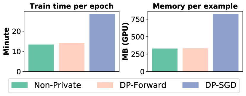
Figure 4 shows the efficiency comparisons on fine-tuning SST-2. The time and storage overheads of our approach (for all possible instances) are almost the same as the non-private baseline and smaller than DP-SGD. It is because we allow batch processing as in the normal fine-tuning – no need to handle per-example gradients. Meanwhile, our normalization and noise sampling/addition are also faster since the size of embeddings is smaller than that of gradients.
5.5. Noisy Pre-training
Pre-training BERT using DP-Forward, aligned with the noisy fine-tuning, does help accuracy. We use SST-2 as an example and perturb the input embedding matrices. We continue pre-training BERT over English WikiCorpus, the dump with about M words, for an epoch. Table 6 shows that we can obtain pp accuracy gains for most choices of , compared to fine-tuning on the original BERT.
Efficiency-wise, DP-Forward pre-training also consumes much fewer resources; e.g., an existing work (Anil et al., 2022) pre-trains BERT-Large (with million parameters) using DP-SGD on Google TPUs, which requires sufficient memory for handling batch sizes of millions.
| Raw BERT | Noisy BERT | ||
|---|---|---|---|
6. Defense against Privacy Threats
Following the recent taxonomy (Song and Raghunathan, 2020), we study MIAs and two new threats of sequence leakage from their embeddings: embedding inversion and attribute inference. We moderately adapt them to suit our context, e.g., upgrading MIAs (Song and Raghunathan, 2020) to sequence-level.
6.1. Threat Models
For MIAs, we follow prior arts (Shokri et al., 2017; Yeom et al., 2018; Song and Raghunathan, 2020) to consider an adversary with only black-box access to an entire (DP-SGD/DP-Forward-trained) pipeline: It can query the prediction results (e.g., each-class probability) of target sequences but cannot access the pipeline weights and architecture; the hidden embeddings are not revealed.
Despite “different” objectives of inverting or inferring (Section 6.3 or 6.4) from embeddings, we consider both threats involving a general adversary with black-box access to the trained pipeline part . It can get the inference-time (clear/noisy) embeddings of target sequences (Song and Raghunathan, 2020). Besides public prior knowledge, it can collect a limited auxiliary dataset , sharing similar attributes to the targets (Song and Raghunathan, 2020).
DP-SGD only offers CDP for training data and does not protect inference-time input.111111One might add the same noise to it as DP-Forward inference, which indeed mitigates the new threats. However, perturbing gradients in training, inherently “mismatches” from perturbing embeddings in inference, deteriorating task performance significantly, e.g., SST-2 accuracy will be reduced to (with a pp drop) at central . What follows intends to empirically confirm a major merit of DP-Forward in protecting against stronger adversaries and threats to both training- and inference-time inputs.
6.2. Membership Inference Attacks
Attack Objective. MIAs predict whether a data point is in the training set (Shokri et al., 2017). They often exploit the disparity in model behavior between training data and unseen data, i.e., poor model generalization due to overfitting (Yeom et al., 2018). Inferring membership at the token/word level, e.g., a sliding window of tokens (Song and Raghunathan, 2020), is not interesting. We consider more realistic MIAs on entire sequences, which can be extended for more devastating attacks, such as extracting verbatim pre-training sequences via black-box access to GPT-2 (Carlini et al., 2021).
Prior arts (Yeom et al., 2018; Song and Mittal, 2021) suggest that threshold-based MIAs using only prediction confidence (Yeom et al., 2018) or entropy (Song and Mittal, 2021) with proper assumptions are comparable to the more sophisticated one (Shokri et al., 2017) based on shadow training. Adapting the confidence-based MIA to our context exploits that a pipeline is fine-tuned by minimizing its prediction loss: The confidence/probability of predicting a training sequence as its true label should be close to . The adversary can then infer a candidate sequence as a member when the confidence for the predicted label output by pipeline is larger than a pre-set threshold :
where is the indicator function. We simply use a fixed for all possible labels in our evaluation, albeit it can be label-dependent.
The second MIA we use is based on the prediction output (i.e., a vector of probabilities) of a training sequence tends to be a one-hot vector, i.e., its entropy should be close to . Similarly, the adversary can infer as a member when its prediction entropy falls below a preset threshold ; otherwise, it is not deemed a member:
for all possible labels . Note that a totally wrong prediction with probability also leads to entropy approaching . We can address it by encoding the information of the ground-truth label of (Song and Mittal, 2021).
Numerical Results. As in (Yu et al., 2021), all the test examples and a random subset of the training examples (as many as the test ones) are evenly split into two subsets (each has half of the training/test examples), one for finding the optimal , and the other for reporting the attack success rates. Given that the training and test examples likely share the same distribution, we randomly drop/replace tokens in the test examples to enlarge the prediction difference to make MIAs easier.
We evaluated the adapted confidence- and entropy-based MIAs on SST-2 fine-tuned by the non-private baseline, DP-Forward, and DP-SGD. For DP-Forward, we investigate five instances, perturbing input embeddings, three encoders’ outputs, and output embeddings. Table 7 presents the results, where success rates within – are shown in bold. Both DP-Forward and DP-SGD can mitigate MIAs effectively. For all choices of , the two MIAs’ success rates on DP-Forward are reduced to (like random guessing) for deeper layers, outperforming DP-SGD by pp at the same privacy level.
| Method | Attack Success Rate | ||
|---|---|---|---|
| Entropy | Confidence | ||
| Non-private baseline | |||
| 1 | DP-SGD | ||
| DP-Forward (Embedding) | |||
| DP-Forward (Encoder 1) | |||
| DP-Forward (Encoder 7) | |||
| DP-Forward (Encoder 11) | |||
| DP-Forward (Output) | |||
| 3 | DP-SGD | ||
| DP-Forward (Embedding) | |||
| DP-Forward (Encoder 1) | |||
| DP-Forward (Encoder 7) | |||
| DP-Forward (Encoder 11) | |||
| DP-Forward (Output) | |||
| 8 | DP-SGD | ||
| DP-Forward (Embedding) | |||
| DP-Forward (Encoder 1) | |||
| DP-Forward (Encoder 7) | |||
| DP-Forward (Encoder 11) | |||
| DP-Forward (Output) | |||
6.3. Embedding Inversion Attacks
Attack Objective. These attacks aim at recovering the raw text as (unordered) tokens from embeddings, highlighting the risk of directly sharing (without noise) even only text embeddings (for training/inference). They have been employed to reconstruct specific patterns, e.g., identity codes and gene segments (Pan et al., 2020).
We first propose a simple token-wise inversion attack to invert (noisy) token embeddings output by the input embedding layer that maps every token in to (Wu et al., 2016). It can be formulated as:
where is the row of noise from (omitted for DP-SGD or the non-private baseline). It returns with its embedding closest to the observed one of via a nearest-neighbor search over .
A token’s hidden embedding from deeper layers encodes more “abstract” contextual information of the entire sequence it belongs to; the token-wise inversion may be less accurate. We thus require a more general attack (Song and Raghunathan, 2020). It first maps the observed (noisy) embedding back to a lower-layer one using a linear least square model and then selects tokens as to minimize the -distance between the lower-layer representation of and the one from :
where is a lower-layer representation function than .
The above minimization is over , larger than the token-wise candidate space. To determine , we first relax the token selection at each position using a continuous vector in , which is then input (with another temperature parameter) to a softmax function to model the probabilities of selecting each token in . We further derive the token embedding by multiplying the relaxed vector (with each entry as a weight) and the original embedding matrix. Finally, we solve it by a gradient-based method (Song and Raghunathan, 2020).
Numerical Results. The gradient-based attack reports the highest recall (or precision) on inverting the lowest-layer (clear) embeddings (Song and Raghunathan, 2020, Figure 2). To show that DP-Forward can mitigate such “strongest” inversion, we implement both (nearest-neighbor and gradient-based) attacks to invert input embeddings, with the public BERT embedding lookup table as prior. We also report their success rates as recall – the ratios of correct recoveries over the raw targets.
Table 8 shows that DP-Forward can reduce their success rates to a relatively low level, most are within . However, DP-SGD fails in defense. The results corroborate our claim: DP-Forward directly adds noise to embeddings, thus mitigating embedding inversion, whereas DP-SGD only perturbs gradients, offering no protection for the (clear) inference-time embeddings of test sequences.
| Nearest Neighbor | Gradient-based | |||||
|---|---|---|---|---|---|---|
| SST-2 | IMDb | QQP | SST-2 | IMDb | QQP | |
| Non-private | ||||||
| DP-SGD | ||||||
| DP-Forward | | | | | | |
6.4. Sensitive Attribute Inference Attacks
Attack Objective. Instead of recovering exact tokens, one can try to infer sensitive attributes about target sequences from their embeddings. The attributes are often statistically unrelated to the training/inference objective but inherent in sequences, e.g., stylometry, implying the text’s authorship for sentiment analysis (Shetty et al., 2018). We are not interested in any global property of an entire corpus (Ganju et al., 2018).
| action | comedy | drama | horror | Overall | |
| Non-private | |||||
| DP-SGD | |||||
| DP-Forward (Embedding) | |||||
| DP-Forward (Encoder 1) | |||||
| DP-Forward (Encoder 7) | |||||
| DP-Forward (Encoder 11) | |||||
| DP-Forward (Output) |
We assume has sequences labeled with sensitive attributes. The adversary can query for the noisy (or clear) embeddings:
where is the set of all possible sensitive attributes of interest, say, authorship. It does not care about non-sensitive attributes.
To infer sensitive attributes, the adversary first trains a classifier on via supervised learning and then uses it for an observed noisy (or clear) embedding to predict of .
Numerical Results. We train a three-layer neural network with a linear head as the classifier to infer the film genre (e.g., ‘horror’) as a sensitive attribute from a movie review using its output embedding. We employ IMDb with k examples ( for training and for validation) as , and SST-2 contributes k examples for testing the classifier. The attack success rates are measured using recall.
We investigate five DP-Forward instances. Table 9 shows that they “reduce” the classifier to majority-class prediction, which returns the majority class (‘action’) on all inputs. In contrast, DP-SGD only reduces success rates moderately compared to the non-private baseline. It is because the embeddings from DP-SGD-trained/noisy models still “lose” some useful information (cf., accuracy drops of DP-SGD inference on embeddings without noise). The results confirm DP-Forward is more effective in thwarting attribute inference.
7. Related Work
7.1. Privacy Threats on LMs and Embeddings
An active line of research (Pan et al., 2020; Song and Raghunathan, 2020; Béguelin et al., 2020; Carlini et al., 2021) discloses severe privacy risks in modern LMs (even used as black-box query “oracles”) concerning their (hidden/output) text embeddings. Song and Raghunathan (Song and Raghunathan, 2020) build a taxonomy of attacks that covers a broader scope than a parallel work (Pan et al., 2020). These attacks include embedding inversion (which can partially recover raw texts), membership inference (establishing the is-in relation between a target and private training data), and inferring sensitive attributes like text authorship from embeddings. A common defense for them is adversarial training, e.g., (Elazar and Goldberg, 2018).
Others (Béguelin et al., 2020; Carlini et al., 2021) study the “memorization” of training data in LMs (a.k.a. membership inference attack). In particular, Carlini et al. (Carlini et al., 2021) define -eidetic memorization, where a string is extractable or memorized if it appears in at most examples. Their black-box attacks on GPT-2 (Radford et al., 2018) can extract verbatim training texts even when (e.g., a name that only appears once is still extractable). A smaller means a higher privacy risk. Beguelin et al. (Béguelin et al., 2020) define differential score and rank as two new metrics for analyzing the update leakage, enabling the recovery of new text used to update LMs. Incorporating DP to address memorization is a promising solution.
7.2. Input (Text/Feature) Perturbation for LDP
SynTF (Weggenmann and Kerschbaum, 2018) synthesizes term-frequency (feature) vectors under LDP, which have limited applications compared to sentence embeddings or text itself. Feyisetan et al. (Feyisetan et al., 2019, 2020) resort to metric-LDP (Alvim et al., 2018), a relaxed variant of LDP with a distance metric (e.g., Euclidean or Hyperbolic), which allows the indistinguishability of outputs to grow proportionally to the inputs’ distance. They first add noise to the outputs of a non-contextualized token embedding model (e.g., GLoVe (Pennington et al., 2014)), which are then projected back to “sanitized” text using the nearest neighbor search as post-processing. In contrast, Yue et al. (Yue et al., 2021) sanitize text by directly sampling token-wise replacements, avoiding adding noise to high-dimensional embeddings. All these works only achieve (variants of) token-level metric-LDP.
To offer sequence-level protection, recent studies (Lyu et al., 2020; Meehan et al., 2022) apply Laplace or exponential mechanism to perturb (the average of) sentence embeddings extracted by an LM (e.g., BERT (Devlin et al., 2019)). Both ensure pure LDP (homogeneously protecting any entire sequence), which may be too stringent and impact utility. In contrast, heterogeneous protection (Feyisetan et al., 2020; Yue et al., 2021) can strategically manage the privacy demands across inputs. Du et al. (Du et al., 2023) achieve metric-LDP (by Purkayastha and planar Laplace mechanisms) at the sequence level (unlike token-level in prior arts (Feyisetan et al., 2020; Yue et al., 2021)). To further boost the utility, they mitigate the dimensional curse via a random-projection-like approach. They also perturb sensitive sequence labels for enhanced privacy. Nevertheless, perturbing different hidden (rather than token or sentence) embeddings inside LM-based NLP pipelines remains unexplored.
7.3. DP-SGD (Variants) in Training LMs
An early attempt (McMahan et al., 2018) uses DP-SGD to train long short-term memory LMs in the federated learning setting. By configuring hyperparameters properly (e.g., setting the batch size to millions), one can even pre-train BERT-Large, an LM with M parameters, using DP-SGD/Adam while achieving acceptable (MLM) accuracy (Anil et al., 2022).
Using the vanilla DP-SGD in pre-training/fine-tuning large LMs leads to significant efficiency and accuracy drops due to the “curse of dimensionality.” Yu et al. (Yu et al., 2021) propose reparametrized gradient perturbation: It first reparameterizes/decomposes each high-rank weight matrix into two low-rank (gradient-carrier) ones with a residual matrix and then only perturbs the two low-rank gradients to alleviate the dimensional curse. The noisy low-rank gradients are finally projected back to update the raw high-rank weights.
Applying reparameterization to every weight in each update is still costly and may introduce instability (e.g., noises are “zoomed up” during the projection). Instead, the follow-up (Yu et al., 2022) builds atop the recent success of parameter-efficient fine-tuning (e.g., LoRA (Hu et al., 2022), Adapter (Houlsby et al., 2019), and Compacter (Mahabadi et al., 2021)): It perturbs the gradients of a much smaller number of additional “plug-in” parameters. However, Li et al. (Li et al., 2022b) empirically show that parameter-efficient fine-tuning is not necessarily better than the full one; they propose ghost clipping, a memory-saving technique (“orthogonal” to dimension reduction), to use DP-SGD in full fine-tuning without instantiating per-example gradients. Despite efficiency/accuracy gains, all these works still only protect training data by perturbing (smaller) gradients.
7.4. DP Mechanisms for Matrix Functions
Gaussian and Laplace mechanisms are typically for scalar-/vector-valued functions (Dwork and Roth, 2014). Vectorizing the outputs and adding i.i.d. noise could generalize them for matrix-valued functions, but the structural information of matrix functions is not exploited. The MVG mechanism (Chanyaswad et al., 2018) is thus devised, which draws directional or non-i.i.d. noise from a matrix Gaussian distribution. It injects less noise into more “informative” output directions for better utility, with only a constraint on the sum of the singular values (determining the noise magnitude) of two covariance matrices. Such a constraint is only a sufficient condition for -DP, which is improved by the follow-up (Yang et al., 2023) with a tighter bound on the singular values.
There also exist mechanisms dedicated to restricted matrix-valued functions. The matrix mechanism (Li et al., 2015) considers a collection of linear counting queries represented by for query matrix and input vector . It still resorts to additive Laplace/Gaussian noise but with an extra transformation solving the min-variance estimation to the noisy . Another very recent study (Ji et al., 2021) focuses on matrix-valued queries with only binary (matrix) outputs. It then devises an exclusive-or (xor) mechanism xor-ing the outputs with noise attributed to a matrix-valued Bernoulli distribution.
8. Conclusion
Pre-trained LMs became pivotal in NLP. Alarmingly, fine-tuning corpora or inference-time inputs face various privacy attacks. The popular DP-SGD only provides limited protection for training data by adding noise to gradients. Raw tokens or sensitive attributes of training/inference data can be inverted or inferred from embeddings in forward-pass computation. Vanilla DP-SGD also imposes high GPU memory and computational burdens but cannot be batched.
We propose DP-Forward, which directly adds noise to embedding matrices derived from the raw training/inference data in the forward pass. Its core is the analytic matrix Gaussian mechanism, a general-purpose tool that owns independent interests. It draws optimal matrix-valued noise from a matrix Gaussian distribution in a dedicated way using a necessary and sufficient condition for DP.
Perturbing embeddings at various positions across multiple layers yields at least two benefits. DP-Forward users are only required to download pipeline parts for deriving noisy embeddings, which is more storage- and time-efficient than deriving noisy gradients. Together with our prior attempts (Yue et al., 2021; Du et al., 2023) at sanitizing input text tokens and output sentence embeddings, we provide a full suite of forward-pass signal sanitization options for users only to share their sanitized data for LM-as-a-Service APIs while protecting privacy.
Beyond the theoretical contribution of two local DP notions and the experimental comparisons with baselines (e.g., GM, MVG, and DP-SGD) across three typical NLP tasks, we investigate the hyperparameter configuration for reproducible validations of DP-Forward’s potential in terms of efficiency, accuracy, and its ability to withstand diverse against diverse attacks.
Altogether, our new perspective leads to a better approach to privacy-aware deep neural network training, challenging the traditional wisdom focusing on gradients. As a new paradigm for local DP in fine-tuning and inference, our work paves the way for a myriad of possibilities for new machine-learning privacy research (Ng and Chow, 2023), e.g., generalization to transformer-based computer vision tasks.
Acknowledgements.
We are grateful to the anonymous reviewers for their comments and Ashwin Machanavajjhala for his comments on a related Ph.D. thesis. Sherman Chow is supported in part by the General Research Funds (CUHK 14209918, 14210319, 14210621), Research Grants Council, University Grants Committee, Hong Kong. Authors at OSU are sponsored in part by NSF IIS , NSF CAREER , and Ohio Supercomputer Center (OSC, 1987). Tianhao Wang is supported in part by National Science Foundation (NSF) with grants CNS- and OAC-.References
- (1)
- Abadi et al. (2016) Martín Abadi, Andy Chu, Ian J. Goodfellow, H. Brendan McMahan, Ilya Mironov, Kunal Talwar, and Li Zhang. 2016. Deep Learning with Differential Privacy. In CCS. 308–318.
- Aboagye et al. (2022) Prince Osei Aboagye, Yan Zheng, Chin-Chia Michael Yeh, Junpeng Wang, Wei Zhang, Liang Wang, Hao Yang, and Jeff M. Phillips. 2022. Normalization of Language Embeddings for Cross-Lingual Alignment. In ICLR (Poster). 32 pages.
- Abowd et al. (2022) John Abowd, Robert Ashmead, Ryan Cumings-Menon, Simson Garfinkel, Micah Heineck, Christine Heiss, Robert Johns, Daniel Kifer, Philip Leclerc, Ashwin Machanavajjhala, Brett Moran, William Sexton, Matthew Spence, and Pavel Zhuravlev. 2022. The 2020 Census Disclosure Avoidance System TopDown Algorithm. Harvard Data Science Review Special Issue 2: Differential Privacy for the 2020 U.S. Census (Jun 24 2022), 77 pages. https://hdsr.mitpress.mit.edu/pub/7evz361i.
- Alvim et al. (2018) Mário S. Alvim, Konstantinos Chatzikokolakis, Catuscia Palamidessi, and Anna Pazii. 2018. Invited Paper: Local Differential Privacy on Metric Spaces: Optimizing the Trade-Off with Utility. In CSF. 262–267.
- Anil et al. (2022) Rohan Anil, Badih Ghazi, Vineet Gupta, Ravi Kumar, and Pasin Manurangsi. 2022. Large-Scale Differentially Private BERT. In Findings of EMNLP. 6481–6491.
- Ba et al. (2016) Lei Jimmy Ba, Jamie Ryan Kiros, and Geoffrey E. Hinton. 2016. Layer Normalization. arXiv:1607.06450.
- Balle and Wang (2018) Borja Balle and Yu-Xiang Wang. 2018. Improving the Gaussian Mechanism for Differential Privacy: Analytical Calibration and Optimal Denoising. In ICML. 403–412.
- Béguelin et al. (2020) Santiago Zanella Béguelin, Lukas Wutschitz, Shruti Tople, Victor Rühle, Andrew Paverd, Olga Ohrimenko, Boris Köpf, and Marc Brockschmidt. 2020. Analyzing Information Leakage of Updates to Natural Language Models. In CCS. 363–375.
- Bonawitz et al. (2017) Kallista A. Bonawitz, Vladimir Ivanov, Ben Kreuter, Antonio Marcedone, H. Brendan McMahan, Sarvar Patel, Daniel Ramage, Aaron Segal, and Karn Seth. 2017. Practical Secure Aggregation for Privacy-Preserving Machine Learning. In CCS. 1175–1191.
- Bu et al. (2019) Zhiqi Bu, Jinshuo Dong, Qi Long, and Weijie J. Su. 2019. Deep Learning with Gaussian Differential Privacy. arXiv:1911.11607.
- Busa-Fekete et al. (2021) Robert Istvan Busa-Fekete, Andres Munoz Medina, Umar Syed, and Sergei Vassilvitskii. 2021. On the pitfalls of label differential privacy. In NeurIPS Workshop. 6 pages.
- Carlini et al. (2019) Nicholas Carlini, Chang Liu, Úlfar Erlingsson, Jernej Kos, and Dawn Song. 2019. The Secret Sharer: Evaluating and Testing Unintended Memorization in Neural Networks. In USENIX Security. 267–284.
- Carlini et al. (2021) Nicholas Carlini, Florian Tramèr, Eric Wallace, Matthew Jagielski, Ariel Herbert-Voss, Katherine Lee, Adam Roberts, Tom B. Brown, Dawn Song, Úlfar Erlingsson, Alina Oprea, and Colin Raffel. 2021. Extracting Training Data from Large Language Models. In USENIX Security. 2633–2650.
- Chanyaswad et al. (2018) Thee Chanyaswad, Alex Dytso, H. Vincent Poor, and Prateek Mittal. 2018. MVG Mechanism: Differential Privacy under Matrix-Valued Query. In CCS. 230–246.
- Chase and Chow (2009) Melissa Chase and Sherman S. M. Chow. 2009. Improving privacy and security in multi-authority attribute-based encryption. In CCS. 121–130.
- Chaudhuri and Hsu (2011) Kamalika Chaudhuri and Daniel J. Hsu. 2011. Sample Complexity Bounds for Differentially Private Learning. In COLT. 155–186.
- Chaudhuri and Monteleoni (2008) Kamalika Chaudhuri and Claire Monteleoni. 2008. Privacy-preserving logistic regression. In NIPS. 289–296.
- Chaudhuri et al. (2011) Kamalika Chaudhuri, Claire Monteleoni, and Anand D. Sarwate. 2011. Differentially Private Empirical Risk Minimization. J. Mach. Learn. Res. 12 (2011), 1069–1109.
- Dasoulas et al. (2021) George Dasoulas, Kevin Scaman, and Aladin Virmaux. 2021. Lipschitz normalization for self-attention layers with application to graph neural networks. In ICML, Vol. 139. 2456–2466.
- Devlin et al. (2019) Jacob Devlin, Ming-Wei Chang, Kenton Lee, and Kristina Toutanova. 2019. BERT: Pre-training of Deep Bidirectional Transformers for Language Understanding. In NAACL-HLT. 4171–4186.
- Du et al. (2023) Minxin Du, Xiang Yue, Sherman S. M. Chow, and Huan Sun. 2023. Sanitizing Sentence Embeddings (and Labels) for Local Differential Privacy. In WWW. 2349–2359.
- Dwork et al. (2006) Cynthia Dwork, Frank McSherry, Kobbi Nissim, and Adam D. Smith. 2006. Calibrating Noise to Sensitivity in Private Data Analysis. In TCC. 265–284.
- Dwork and Roth (2014) Cynthia Dwork and Aaron Roth. 2014. The Algorithmic Foundations of Differential Privacy. Found. Trends Theor. Comput. Sci. 9, 3-4 (2014), 211–407.
- Elazar and Goldberg (2018) Yanai Elazar and Yoav Goldberg. 2018. Adversarial Removal of Demographic Attributes from Text Data. In EMNLP. 11–21.
- Erlingsson et al. (2019) Úlfar Erlingsson, Vitaly Feldman, Ilya Mironov, Ananth Raghunathan, Kunal Talwar, and Abhradeep Thakurta. 2019. Amplification by Shuffling: From Local to Central Differential Privacy via Anonymity. In SODA. 2468–2479.
- Esmaeili et al. (2021) Mani Malek Esmaeili, Ilya Mironov, Karthik Prasad, Igor Shilov, and Florian Tramèr. 2021. Antipodes of Label Differential Privacy: PATE and ALIBI. In NeurIPS. 6934–6945.
- Face (2023) Hugging Face. 2023. BERT base model (uncased). https://huggingface.co/bert-base-uncased, last accessed: September 12, 2023.
- Feyisetan et al. (2020) Oluwaseyi Feyisetan, Borja Balle, Thomas Drake, and Tom Diethe. 2020. Privacy- and Utility-Preserving Textual Analysis via Calibrated Multivariate Perturbations. In WSDM. 178–186.
- Feyisetan et al. (2019) Oluwaseyi Feyisetan, Tom Diethe, and Thomas Drake. 2019. Leveraging Hierarchical Representations for Preserving Privacy and Utility in Text. In ICDM. 210–219.
- Ganju et al. (2018) Karan Ganju, Qi Wang, Wei Yang, Carl A. Gunter, and Nikita Borisov. 2018. Property Inference Attacks on Fully Connected Neural Networks using Permutation Invariant Representations. In CCS. 619–633.
- Ghazi et al. (2021) Badih Ghazi, Noah Golowich, Ravi Kumar, Pasin Manurangsi, and Chiyuan Zhang. 2021. Deep Learning with Label Differential Privacy. In NeurIPS. 27131–27145.
- Gopi et al. (2021) Sivakanth Gopi, Yin Tat Lee, and Lukas Wutschitz. 2021. Numerical Composition of Differential Privacy. In NeurIPS. 11631–11642.
- Hall et al. (2013) Robert J. Hall, Larry A. Wasserman, and Alessandro Rinaldo. 2013. Random Differential Privacy. J. Priv. Confidentiality 4, 2 (2013), 43–59.
- Horn and Johnson (2012) Roger A. Horn and Charles R. Johnson. 2012. Matrix Analysis, 2nd Ed. Cambridge University Press, N/A.
- Houlsby et al. (2019) Neil Houlsby, Andrei Giurgiu, Stanislaw Jastrzebski, Bruna Morrone, Quentin de Laroussilhe, Andrea Gesmundo, Mona Attariyan, and Sylvain Gelly. 2019. Parameter-Efficient Transfer Learning for NLP. In ICML, Vol. 97. 2790–2799.
- Hu et al. (2022) Edward J. Hu, Yelong Shen, Phillip Wallis, Zeyuan Allen-Zhu, Yuanzhi Li, Shean Wang, Lu Wang, and Weizhu Chen. 2022. LoRA: Low-Rank Adaptation of Large Language Models. In ICLR (Poster). 13 pages.
- Ji et al. (2021) Tianxi Ji, Pan Li, Emre Yilmaz, Erman Ayday, Yanfang Ye, and Jinyuan Sun. 2021. Differentially Private Binary- and Matrix-Valued Data Query: An XOR Mechanism. Proc. VLDB Endow. 14, 5 (2021), 849–862.
- Kasiviswanathan et al. (2008) Shiva Prasad Kasiviswanathan, Homin K. Lee, Kobbi Nissim, Sofya Raskhodnikova, and Adam D. Smith. 2008. What Can We Learn Privately?. In FOCS. 531–540.
- Kim et al. (2021) Hyunjik Kim, George Papamakarios, and Andriy Mnih. 2021. The Lipschitz Constant of Self-Attention. In ICML, Vol. 139. 5562–5571.
- Laurent and Massart (2000) Beatrice Laurent and Pascal Massart. 2000. Adaptive estimation of a quadratic functional by model selection. The Annals of Statistics 28, 5 (2000), 1302–1338.
- Lécuyer et al. (2019) Mathias Lécuyer, Vaggelis Atlidakis, Roxana Geambasu, Daniel Hsu, and Suman Jana. 2019. Certified Robustness to Adversarial Examples with Differential Privacy. In S&P. 656–672.
- Lehman et al. (2021) Eric Lehman, Sarthak Jain, Karl Pichotta, Yoav Goldberg, and Byron C. Wallace. 2021. Does BERT Pretrained on Clinical Notes Reveal Sensitive Data?. In NAACL-HLT. 946–959.
- Li et al. (2015) Chao Li, Gerome Miklau, Michael Hay, Andrew McGregor, and Vibhor Rastogi. 2015. The matrix mechanism: optimizing linear counting queries under differential privacy. VLDB J. 24, 6 (2015), 757–781.
- Li et al. (2022a) Jing Li, Aixin Sun, Jianglei Han, and Chenliang Li. 2022a. A Survey on Deep Learning for Named Entity Recognition. IEEE Trans. Knowl. Data Eng. 34, 1 (2022), 50–70.
- Li et al. (2022b) Xuechen Li, Florian Tramèr, Percy Liang, and Tatsunori Hashimoto. 2022b. Large Language Models Can Be Strong Differentially Private Learners. In ICLR. 30 pages.
- Lyu et al. (2020) Lingjuan Lyu, Xuanli He, and Yitong Li. 2020. Differentially Private Representation for NLP: Formal Guarantee and An Empirical Study on Privacy and Fairness. In Findings of EMNLP. 2355–2365.
- Maas et al. (2011) Andrew L. Maas, Raymond E. Daly, Peter T. Pham, Dan Huang, Andrew Y. Ng, and Christopher Potts. 2011. Learning Word Vectors for Sentiment Analysis. In ACL. 142–150.
- Mahabadi et al. (2021) Rabeeh Karimi Mahabadi, James Henderson, and Sebastian Ruder. 2021. Compacter: Efficient Low-Rank Hypercomplex Adapter Layers. In NeurIPS. 1022–1035.
- McDermott and Forsyth (2016) James McDermott and Richard S. Forsyth. 2016. Diagnosing a disorder in a classification benchmark. Pattern Recognit. Lett. 73 (2016), 41–43.
- McMahan et al. (2018) H. Brendan McMahan, Daniel Ramage, Kunal Talwar, and Li Zhang. 2018. Learning Differentially Private Recurrent Language Models. In ICLR (Poster). 14 pages.
- Meehan et al. (2022) Casey Meehan, Khalil Mrini, and Kamalika Chaudhuri. 2022. Sentence-level Privacy for Document Embeddings. In ACL. 3367–3380.
- Min et al. (2022) Sewon Min, Xinxi Lyu, Ari Holtzman, Mikel Artetxe, Mike Lewis, Hannaneh Hajishirzi, and Luke Zettlemoyer. 2022. Rethinking the Role of Demonstrations: What Makes In-Context Learning Work?. In EMNLP. 11048–11064.
- Mironov (2017) Ilya Mironov. 2017. Rényi Differential Privacy. In CSF. 263–275.
- Ng and Chow (2023) Lucien K. L. Ng and Sherman S. M Chow. 2023. SoK: Cryptographic Neural-Network Computation. In S&P. 497–514.
- OSC (1987) OSC. 1987. Ohio Supercomputer Center. http://osc.edu/ark:/19495/f5s1ph73
- Pan et al. (2020) Xudong Pan, Mi Zhang, Shouling Ji, and Min Yang. 2020. Privacy Risks of General-Purpose Language Models. In S&P. 1314–1331.
- Pennington et al. (2014) Jeffrey Pennington, Richard Socher, and Christopher D. Manning. 2014. Glove: Global Vectors for Word Representation. In EMNLP. 1532–1543.
- Qu et al. (2021) Chen Qu, Weize Kong, Liu Yang, Mingyang Zhang, Michael Bendersky, and Marc Najork. 2021. Natural Language Understanding with Privacy-Preserving BERT. In CIKM. 1488–1497.
- Radford et al. (2018) Alec Radford, Karthik Narasimhan, Tim Salimans, and Ilya Sutskever. 2018. Improving language understanding by generative pre-training. OpenAI Report.
- Radford et al. (2019) Alec Radford, Jeff Wu, Rewon Child, David Luan, Dario Amodei, and Ilya Sutskever. 2019. Language Models are Unsupervised Multitask Learners. OpenAI Report.
- Reimers and Gurevych (2019) Nils Reimers and Iryna Gurevych. 2019. Sentence-BERT: Sentence Embeddings using Siamese BERT-Networks. In EMNLP-IJCNLP. 3980–3990.
- Shetty et al. (2018) Rakshith Shetty, Bernt Schiele, and Mario Fritz. 2018. A4NT: Author Attribute Anonymity by Adversarial Training of Neural Machine Translation. In USENIX Security. 1633–1650.
- Shokri et al. (2017) Reza Shokri, Marco Stronati, Congzheng Song, and Vitaly Shmatikov. 2017. Membership Inference Attacks Against Machine Learning Models. In S&P. 3–18.
- Song and Raghunathan (2020) Congzheng Song and Ananth Raghunathan. 2020. Information Leakage in Embedding Models. In CCS. 377–390.
- Song and Mittal (2021) Liwei Song and Prateek Mittal. 2021. Systematic Evaluation of Privacy Risks of Machine Learning Models. In USENIX Security. 2615–2632.
- Steinke (2022) Thomas Steinke. 2022. Composition of Differential Privacy & Privacy Amplification by Subsampling. arXiv:2210.00597.
- Sweeney (2015) Latanya Sweeney. 2015. Only You, Your Doctor, and Many Others May Know. Technology Science 2015092903, 9 (2015), 29.
- Vaswani et al. (2017) Ashish Vaswani, Noam Shazeer, Niki Parmar, Jakob Uszkoreit, Llion Jones, Aidan N. Gomez, Lukasz Kaiser, and Illia Polosukhin. 2017. Attention is All You Need. In NeurIPS. 5998–6008.
- Wang et al. (2019) Alex Wang, Amanpreet Singh, Julian Michael, Felix Hill, Omer Levy, and Samuel R. Bowman. 2019. GLUE: A Multi-Task Benchmark and Analysis Platform for Natural Language Understanding. In ICLR (Poster). 20 pages.
- Warner (1965) Stanley L Warner. 1965. Randomized Response: A Survey Technique for Eliminating Evasive Answer Bias. JASA 60, 309 (1965), 63–69.
- Weggenmann and Kerschbaum (2018) Benjamin Weggenmann and Florian Kerschbaum. 2018. SynTF: Synthetic and Differentially Private Term Frequency Vectors for Privacy-Preserving Text Mining. In SIGIR. 305–314.
- Wu et al. (2023) Ruihan Wu, Jin Peng Zhou, Kilian Q. Weinberger, and Chuan Guo. 2023. Does Label Differential Privacy Prevent Label Inference Attacks?. In AISTAST. 4336–4347.
- Wu et al. (2016) Yonghui Wu, Mike Schuster, Zhifeng Chen, Quoc V. Le, Mohammad Norouzi, Wolfgang Macherey, Maxim Krikun, Yuan Cao, Qin Gao, Klaus Macherey, Jeff Klingner, Apurva Shah, Melvin Johnson, Xiaobing Liu, Lukasz Kaiser, Stephan Gouws, Yoshikiyo Kato, Taku Kudo, Hideto Kazawa, Keith Stevens, George Kurian, Nishant Patil, Wei Wang, Cliff Young, Jason Smith, Jason Riesa, Alex Rudnick, Oriol Vinyals, Greg Corrado, Macduff Hughes, and Jeffrey Dean. 2016. Google’s Neural Machine Translation System: Bridging the Gap between Human and Machine Translation. arXiv:1609.08144.
- Yang et al. (2021) Jungang Yang, Liyao Xiang, Weiting Li, Wei Liu, and Xinbing Wang. 2021. Improved Matrix Gaussian Mechanism for Differential Privacy. arXiv:2104.14808.
- Yang et al. (2023) Jungang Yang, Liyao Xiang, Jiahao Yu, Xinbing Wang, Bin Guo, Zhetao Li, and Baochun Li. 2023. Matrix Gaussian Mechanisms for Differentially-Private Learning. IEEE Trans. Mob. Comput. 22, 2 (2023), 1036–1048.
- Yeom et al. (2018) Samuel Yeom, Irene Giacomelli, Matt Fredrikson, and Somesh Jha. 2018. Privacy Risk in Machine Learning: Analyzing the Connection to Overfitting. In CSF. 268–282.
- Yousefpour et al. (2021) Ashkan Yousefpour, Igor Shilov, Alexandre Sablayrolles, Davide Testuggine, Karthik Prasad, Mani Malek, John Nguyen, Sayan Ghosh, Akash Bharadwaj, Jessica Zhao, Graham Cormode, and Ilya Mironov. 2021. Opacus: User-Friendly Differential Privacy Library in PyTorch. arXiv:2109.12298.
- Yu et al. (2022) Da Yu, Saurabh Naik, Arturs Backurs, Sivakanth Gopi, Huseyin A. Inan, Gautam Kamath, Janardhan Kulkarni, Yin Tat Lee, Andre Manoel, Lukas Wutschitz, Sergey Yekhanin, and Huishuai Zhang. 2022. Differentially Private Fine-tuning of Language Models. In ICLR (Poster). 19 pages.
- Yu et al. (2021) Da Yu, Huishuai Zhang, Wei Chen, Jian Yin, and Tie-Yan Liu. 2021. Large Scale Private Learning via Low-rank Reparametrization. In ICML. 12208–12218.
- Yue et al. (2021) Xiang Yue, Minxin Du, Tianhao Wang, Yaliang Li, Huan Sun, and Sherman S. M. Chow. 2021. Differential Privacy for Text Analytics via Natural Text Sanitization. In Findings of ACL/IJCNLP. 3853–3866.
- Zhou et al. (2022) Mingxun Zhou, Tianhao Wang, T.-H. Hubert Chan, Giulia Fanti, and Elaine Shi. 2022. Locally Differentially Private Sparse Vector Aggregation. In S&P. 422–439.
Appendix A Token-level DP-Forward
A.1. Definition and Related Notions
Definition 0 (Token-level SeqLDP).
For , fulfills token-level -SeqLDP, if that differ in any single token but with the same , and any possible output subset ,
Despite a token-level notion, our experiments (Appendix A.3) show that when is only the input embedding layer, our token-level SeqLDP designs can also effectively mitigate MIAs on entire sequences, with up to pp accuracy gains at the same choices of . It is not necessarily weaker than sequence-level CDP (as offered by DP-SGD). One might doubt its usefulness since two neighboring sequences may be too similar. Nevertheless, there are cases where a sentence, e.g., “How’s it going” may not matter in a bigger unit (paragraph/essay) of the training data either. Moreover, a token (e.g., yes/no) can play a crucial role, e.g., in named entity recognition (Li et al., 2022a). Our LDP guarantee is for any such two sequences, covering the wide spectrum between “too similar” and radically different cases.
Note that weakening privacy notions by itself is not our goal121212As a related example, in image classification, PixelDP (Lécuyer et al., 2019) has been proposed for a DP notion defined upon pixels. Its motivation is robustness to adversarial examples.. Protection at the token level has been studied under metric-DP (Feyisetan et al., 2020; Qu et al., 2021), a relaxation of LDP. They require even much larger , say, . Our goal of studying token-level SeqLDP is to narrow the gap between theory and practice, i.e., provable privacy notions tailored to the protection targets (the first few layers vs. the whole pipeline).
A.2. Two Token-level SeqLDP Designs
For token-level SeqLDP, we need to bound a “new” , which should be tight and smaller than the one over , hence producing smaller noise for better utility at meaningful token-level . It is still non-trivial since , except for being the input embedding layer, may differ in every entry for even . One could also normalize the entire for , which “degenerates” to the token-level SeqLDP. Instead, we tailor two designs to estimate a tighter than the “general” one for only the input embedding layer and the first two layers, respectively. Specifically, we employ row-wise normalization and the Lipschitz continuity (Kim et al., 2021).
After the Input Embedding Layer. When is only the input embedding layer, we work on each row independently: , where is vector -norm. As a token only affects one row, we have , independent of whether the embedding layer will be updated. Again with , we can draw noise .
In the First MHA Sub-layer. The second option could be adding right after the first MHA sub-layer: , where is the concatenation of . Yet, it is non-trivial to estimate of as , let alone , is not Lipschitz (Kim et al., 2021).
Definition 0 (Lipschitz Continuity).
Given two metric spaces and , a function is Lipschitz continuous (-Lipschitz) if there exists a constant ,
The smallest is the Lipschitz constant, denoted by .
We consider that is the space of row-wise normalized matrices in , is the output space of or , and (or -norm ). generalizes since it focuses on any two inputs rather than just neighboring ones, allowing us to estimate an upper bound for given .
The non-Lipschitz continuity stems from the non-linear Softmax activation, which takes pairwise dot products as input (Kim et al., 2021). To make MHA Lipschitz, one might apply pairwise -distances (hence called -MHA) (Kim et al., 2021) or add a normalization step called LipschitzNorm (Dasoulas et al., 2021) in . Unfortunately, estimating of -MHA needs to solve an intractable optimization problem, and LipschitzNorm is ill-suited for the high-dimensional BERT attention.
Instead of adding to the outputs of or , we can shift inside , where estimating or is feasible, e.g., the linear maps used to derive matrices. Considering a linear map with and , the -norm is the largest singular value (Kim et al., 2021). When generalizing for any two matrices , we can estimate
We can now respectively derive the noisy matrices for . The first step is to draw noise given . It requires us to either estimate on the fly via power iteration or fix the linear maps in each forward pass of fine-tuning or inference. We then compute , which are reshaped into matrices of size for .
Theorem 3.
The two instances (with row-wise normalization) for fine-tuning or inference fulfill token-level -(Seq)LDP.
The proof is equivalent to our approach for (Seq)LDP. One just needs to compute properly, and we did.
Discussion.
For minimal changes to the pipeline, we adopt the raw WordPiece (Wu et al., 2016), which splits text into sub-words; using word-level tokenization yields word-level (Seq)LDP. Our notion can also extend to phrase-level (Seq)LDP by directly using the group privacy (Dwork and Roth, 2014) or dedicatedly computing the -sensitivity smaller than for two sequences differing in (consecutive) tokens. Typically, is small since a few tokens are enough for most sensitive information. One could also add noise deeper in a pipeline using , where is function composition . We then need to estimate of each (component of) sub-layer. For example, has two linear maps and with in between, where of is . For , its is bounded by since with as the rank. We can also estimate of from its Lipschitz constant (Kim et al., 2021). When is composed of more layers, we can only get a looser estimation on the final . Hence, our general recommendation is to add noise early when estimating a tight is feasible.

A.3. More Experiment Results
We also study the privacy-accuracy tradeoff on all three tasks for our two token-level SeqLDP designs when tuning local . The results are compared with the non-private baseline and fine-tuning using MVG noise. Figure 5 shows task accuracy increases with . Perturbing input embeddings for token-level (vs. sequence-level) SeqLDP can achieve remarkable accuracy gain, e.g., vs. for IMDb.
We evaluate the two MIAs on SST-2 fine-tuned by our two token-level SeqLDP instances. Table 10 shows the results, with success rates within (like random guessing) bolded. Even if the provable guarantee is at the token level, our instances can notably reduce the success rates of the confidence-based attack by pp and the entropy-based one by pp, compared to the non-private baseline.
| Local | Method | Attack Success Rate | |
|---|---|---|---|
| Entropy | Confidence | ||
| Non-private baseline | |||
| 8 | DP-Forward (Embedding) | ||
| DP-Forward (Attention) | |||
| 16 | DP-Forward (Embedding) | ||
| DP-Forward (Attention) | |||
| 24 | DP-Forward (Embedding) | ||
| DP-Forward (Attention) | |||
Appendix B Relevant Matrix Algebra
Proposition 0.
Proof.
For the numerator part in Eq. (1), we have
where denotes the matrix trace. Denote
We compute
which is a similar matrix of , and hence . So, the two PDFs are equivalent since
| ∎ |
Theorem 2 (Singular Value Decomposition or SVD (Horn and Johnson, 2012)).
A matrix can be decomposed as , where and are unitary, and is an diagonal matrix whose diagonal entries are ordered singular values of , denoted by (or simply ) with .
Lemma 0.
Given a matrix and two orthogonal matrices , we have ; is immune to the pre- and post-orthogonal transformation.
Proof.
We first prove that by
and similarly we can prove that . ∎
Lemma 0.
For , , where is the singular value of and .
Proof.
The SVD of is . By Lemma 3, we have
| ∎ |
Lemma 0 (Lemma (Yang et al., 2021)).
Given matrices , we have where is the singular value, and .
Proof.
With SVD, are decomposed as
Based on Lemma 4, we have
where and are still two unitary matrices. We further have
where . Hence, we need to show
| (7) |
Following the strategy in (Yang et al., 2021) (cf. Eq. (29), (30)), we rewrite and using non-negative values and s.t.
For , we denote , if ; , otherwise. Then, we transform the Eq. (7) as
Since are non-negative, we only need to show
| (8) |
However, the original proof (Yang et al., 2021) has two issues: i) is not considered, and ii) the commutative law of matrix multiplication in Eq. (35) does not hold as in Eq. (34) is not a standard diagonal matrix. To address them, we have
We then denote a sub-matrix for of . With SVD of , we have
The last inequality is due to for (Horn and Johnson, 2012). So, Inequality (8) holds. ∎
Appendix C Proofs for Our Analytic Matrix Gaussian Mechanism
Proof of Lemma 4.
Recall that with , the probability of is
Similarly, we can compute . By plugging them into , and let ,
where is the vectorization of a matrix and denotes the inner product. For easy presentation, we denote and , and then we re-write
Given Lemma 7, with each entry i.i.d. drawn from . is thus the -weighted sum of i.i.d. Gaussian random variables, which is a Gaussian variable131313en.wikipedia.org/wiki/Sum_of_normally_distributed_random_variables too. So , . ∎
Proof of Lemma 5.
With Lemma 4 and the CDF, we have
where we used and the symmetry of the standard normal distribution .
A similar argument applied to yields
| ∎ |
Proof of Theorem 6.
The proof boils down to two directions. From -DP (Theorem 3) to Theorem 6, the proof directly follows from all the derivations in Section 4.2. For the inverse direction, it is sufficient to show that holds for given Theorem 6. In particular, for , we have
where the first inequality is due to Lemma 5, the second one holds since and are the smallest singular values among the others, and the third one is from Theorem 6. ∎