Downlink Performance of Cell-Free Massive MIMO for LEO Satellite Mega-Constellation
Abstract
Low-earth orbit (LEO) satellite communication (SatCom) has emerged as a promising technology for improving wireless connectivity in global areas. Cell-free massive multiple-input multiple-output (CF-mMIMO), an architecture recently proposed for next-generation networks, has yet to be fully explored for LEO satellites. In this paper, we investigate the downlink performance of a CF-mMIMO LEO SatCom network, where many satellite access points (SAPs) simultaneously serve the corresponding ground user terminals (UTs). Using tools from stochastic geometry, we model the locations of SAPs and UTs on surfaces of concentric spheres using Poisson point processes (PPPs) and present expressions based on linear minimum-mean-square-error (LMMSE) channel estimation and conjugate beamforming. Then, we derive the coverage probabilities in both fading and non-fading scenarios, with significant system parameters such as the Nakagami fading parameter, number of UTs, number of SAPs, orbital altitude, and service range brought by the dome angle. Finally, the analytical model is verified by extensive Monte Carlo simulations. Simulation results show that stronger line-of-sight (LoS) effects and a more comprehensive service range of the UT bring higher coverage probability despite existing multi-user interference. Moreover, we found that there exist optimal numbers of UTs for different orbital altitudes and dome angles, which provides valuable system design insights.
Index Terms:
Satellite-terrestrial communications, low-earth orbit (LEO) satellite, cell-free massive MIMO, coverage probability, stochastic geometry.I Introduction
The advancement of wireless communications and the explosion of high-data-rate demands have led to the expansion of network coverage, which is currently supported by terrestrial networks (TNs). As an essential component of non-terrestrial networks (NTNs), satellite communication (SatCom) is a critical enabler to realize the continuous and ubiquitous connectivity provision, especially in areas with inadequate wireless access [2]. In recent years, low-earth orbit (LEO) satellites, typically located at altitudes between km and km, have gained broad research interests due to their potential to provide worldwide Internet access with improved data rates [3]. Compared with the medium-earth orbit (MEO) or geostationary-earth orbit (GEO) counterparts, LEO satellites are more advantageous due to relatively shorter signal propagation delay, decreased path-loss and power consumption, and lower production and launch costs [4].
In the LEO SatCom network, multi-beam transmission techniques have been widely used to obtain higher throughput and data rates for numerous user terminals (UTs) [5]. One possible utilization of multi-beam transmission in SatCom is its integration with massive multiple-input multiple-output (MIMO) [6], an enabling and widely adopted technology for the fifth-generation (5G) and beyond communication systems. In massive MIMO (mMIMO)-enhanced LEO SatCom networks, significantly higher data rates can be achieved than their traditional single-beam counterparts [7]. However, similar to inter-cell interference of small cells in TNs with collocated mMIMO, inter-satellite interference in NTNs exists due to the service area boundary and causes a severe performance downgrade for served UTs[8]. Therefore, the current satellite network, where a single satellite serves multiple UTs with potential overlap from neighboring satellite coverage areas, may be inadequate for UTs requiring high levels of coverage and data rates. This has directed our research toward a distributed mMIMO network that is theoretically well-suited for SatCom, i.e., cell-free (CF) mMIMO LEO SatCom networks.
Stochastic geometry is a proper mathematical tool for analyzing and evaluating network performance, such as coverage probability, desired signal, and interference statistics from a system-level perspective [9]. Specifically, coverage analysis research has become more tractable, such as the coverage probability in [10, 11, 12] for TNs and in SatCom [12, 13] for NTNs. However, the aforementioned works fail to account for the combined impacts of critical factors such as beamforming, fading parameters, number of satellites, and their orbital altitudes in CF-mMIMO LEO SatCom networks. Since coverage probability is functionally related to these factors, it can be expressed in closed-form equations. Inspired by these observations, this paper develops an analytical model for the coverage and capacity of CF-mMIMO LEO SatCom networks using stochastic geometry. These functional mapping relationships can significantly reduce computational complexity compared to system-level simulations.
I-A Related Works
Many papers have studied the performance of LEO satellite networks. The coverage probability for downlink transmissions was investigated in [14], where satellite locations were distributed as a binomial point process (BPP). However, crucial instruments such as the distance distributions of the BPP are more challenging to analyze compared to those of a Poisson point process (PPP) in unbounded space and therefore, PPP-based satellite modeling was adopted in [15]. Many other works also used PPP to model the constellation. For example, ultra-dense LEO satellite constellations were studied in [16] to find the minimized number of satellites while satisfying the backhaul requirement of each UT. The uplink interference and performance of mega satellite constellations were examined in [17, 18] under the impacts of intra-constellation interference. The above work, although similar to our studied network, assumed that each UT was connected to a single satellite, thus overlooking the possibility of satellite cooperation.
The CF-mMIMO system, where each UT is coherently served in the same time-frequency resource block by a large number of geographically-located access points (APs) [19], has gained extensive research attention recently. Although there has been extensive research on CF-mMIMO in TNs such as [20, 21], relatively few studies have explored its application in LEO SatCom. An LEO satellite was initially considered an “add-on” to improve terrestrial CF networks in [22, 23]. However, they fail to introduce the CF-mMIMO architecture to large-scale LEO satellite networks. The authors in [24, 25] integrated CF-mMIMO into LEO satellite networks and developed an optimization framework to improve spectral efficiency. The benefits of CF-mMIMO in LEO satellite networks were further evaluated in [26] for broadband connectivity with multi-antenna satellites and handheld devices. In addition, the CF-mMIMO SatCom network was also studied from physical layer orthogonal time-frequency-space (OTFS) [27], uplink transmissions with CSI uncertainties [28, 29, 30], and dynamic clustering of satellite access points (SAPs) [31]. However, the above works focused on algorithm designs and assumed that the served UTs were confined in a small region on the earth, neglecting other coverage areas where inter-user interference could arise, as well as downlink interference from non-cooperative satellites. Our previous work [1] examined a basic model for coordinated multi-satellite joint transmissions. However, its reliance on Rayleigh fading and the omission of beamforming and channel estimation strategies made it misaligned with CF-mMIMO and impractical for channels with line-of-sight (LoS) components. Although satellite cooperation was considered in [32, 33], inter-satellite interference persisted, and the lack of beamforming and channel estimation made the structure incompatible. In addition, its tractability decreased as the number of satellites increased.
I-B Contributions and Paper Organization
To thoroughly investigate the downlink performance of CF-mMIMO LEO SatCom networks from a system-level perspective, we incorporate essential factors of satellite networks for analysis using tools from stochastic geometry. The PPP model is adopted to model LEO satellite mega-constellation, providing analytical results with broad applicability and high tractability. Notably, the main contributions of this paper are summarized as follows:
-
•
CF-mMIMO LEO SatCom Network Design: We establish a CF-mMIMO system in the LEO satellite network using stochastic geometry. The locations of SAPs and UTs are modeled on two concentric sphere surfaces, one with the SAPs’ orbital radius and the other with the earth’s radius, respectively, based on two independent homogeneous PPPs. Simulation results demonstrate that the PPP constellation model can fit perfectly with practical constellations. Considering the shape of the earth and the service range, each UT is assigned a group of SAPs for service delivery according to its dome angle.
-
•
Modeling and Analysis: We introduce the related distance distribution for the service links of a typical UT and characterize the average number of UTs served by each SAP. Then, we provide expressions for the distribution of desired signal strength (DSS), the average inter-satellite interference, and the average multi-user interference. The coverage probability of a typical user is then presented accordingly, with both large-scale path-loss and small-scale Nakagami- fading. Furthermore, given the relatively minor impact of multi-path fading components against the long satellite-to-terrestrial distances, we derive the coverage probability for non-fading propagation environments.
-
•
Network Design Insights: We quantitatively analyze the performance of the CF-mMIMO LEO SatCom network concerning key network parameters, including the fading parameter, the service range of CF-mMIMO LEO SatCom network, the total number of SAPs, the number of UTs, and SAPs’ orbital altitudes. We observe that as the dome angle of the typical UT increases, the gain in desired signal power outweighs the increase in received multi-user interference, leading to improved coverage probability, albeit with increased signaling overhead. In addition, an increase in both the orbital altitude and the number of SAPs contributes positively to enhanced coverage performance. While system capacity increases as the number of UTs grows within a certain range, the per-user capacity continues to drop, exhibiting a tradeoff between maximizing system capacity and ensuring minimum throughput for each UT.
The rest of this paper is organized as follows. Section II describes the system model for the studied CF-mMIMO SatCom network, including spatial distributions, channel models, and downlink transmissions. In Section III, we present the statistical properties of the network and derive analytical expressions for the coverage probabilities. Section IV explores the studied system under non-fading channel conditions. Simulations and numerical results are provided in Section V. Finally, Section VI concludes the paper.
Notations: Bold lowercase letters denote column vectors. The superscripts , , and are used to represent conjugate, transpose, and conjugate-transpose, respectively. The real-part operator, expectation operator, the statistical probability, and the Euclidean norm are represented as , , and , respectively. denotes a complex circularly symmetric Gaussian random variable with mean and variance , while denotes that with mean and correlation matrix .
II System Model
In this section, we consider a downlink CF-mMIMO LEO SatCom network over the Nakagami- fading channel, where many SAPs simultaneously serve the UTs on the earth’s surface. For the sake of analysis, each SAP and each UT are equipped with a single antenna111In this paper, both SAPs and UTs can be extended for multiple-antenna scenarios. Our results can serve as a baseline for coverage analysis in multi-antenna models of SAPs or UTs, which is left for future work. Following the basic principle of CF-mMIMO, SAPs are connected to a central server (CS) through high-speed optical inter-satellite links (OISLs), known as backhaul links, to exchange necessary control signals for cooperative transmissions of SAPs222While backhauling system limitations, such as propagation delay and link capacity, are significant concerns, this paper specifically focuses on the access links, particularly the connections between SAPs and ground UTs.. The CS can be deployed on a central satellite, e.g., a GEO satellite, with sufficient power and computing capabilities, following a similar mechanism as in [24, 25, 26, 31, 32].
II-A Spatial Distribution Model
Denote the radius of the earth as , and that of a sphere where the SAPs are located as . An illustration of PPP-distributed satellites and PPP-distributed UTs are shown in Fig. 1(a). The distributions of UTs and SAPs are independent and each follows a homogeneous spherical Poisson point process (SPPPs). In a practical constellation such as Starlink, the distribution of satellites is correlated. For comparison, we simulate the Starlink constellations with random and fixed initial states, respectively. Note that in a random initial state shown in Fig. 1(b), the initial position and orbital parameters of each satellite are randomly distributed within a certain range, which can simulate the randomness of constellations at the time of deployment. This is very similar to the constellation in a practical constellation. In a fixed initial state shown in Fig. 1(c), the initial position and orbital parameters of all satellites are set in advance and strictly fixed to represent the ideal precise deployment situation. The satellites follow strict geometric symmetries in their orbital planes and phases in order to minimize relative deviations between satellites. Intuitively, the PPP model can perfectly simulate a practical constellation by setting a random initial state, which will be verified in Section V.
On this basis, we assume that there are SAPs in the constellation at the same orbital altitude , and there are a total of UTs on the earth surface that need to be served by the CF-mMIMO SatCom network. Taking the mean of the Poisson random variable, the PPP density of UTs and that of SAPs is approximated by and , respectively.
II-B Path-Loss and Channel Model
For the satellite-terrestrial signal transmissions, both large-scale path-loss attenuation and small-scale fading are taken into account. Specifically, a valid assumption is that the fading channel between every two links is assumed to be uncorrelated since SAPs are geographically distributed on the sphere . We denote the channel coefficient between the -th SAP and the -th UT as
| (1) |
where denotes the large-scale fading and is the small-scale fading333Similar to [14, 15, 16, 17, 18], the perfect CSI is assumed. The derived expressions for the coverage probability provide upper-bound performance for the system. However, in this paper, more pilots will bring better CSI. We will evaluate how the number of pilots influences the DSS in Section V.. For large-scale fading, can be represented using a distance-dependent model, i.e. , where is the path-loss at a reference distance, and is the path-loss exponent. Then, the effective antenna gain is denoted as
| (2) |
where and are the transmit antenna gain of the SAP and the receive antenna gain of the UT, is the speed of light, and is the carrier frequency. The small-scale fading is modeled via the Nakagami- distribution, whose probability density function (PDF) is given by
| (3) |
with , and for integer . The Nakagami- model is selected because of its adaptation to various small-scale fading conditions, e.g. Rayleigh channel when and Rician- channel when [15]. We also have . Note that Shadowed-Rician (SR) fading can also be approximated by Nakagami- fading [18]. Moreover, changing this parameter makes it suitable for describing various channels, as it allows one to model the signal propagation conditions from severe to moderate.
II-C Uplink Training
In a CF-mMIMO system, the propagation channels are considered to be piecewise constant during each coherence time period and frequency coherence interval. Therefore, training must be conducted within each time-frequency coherence block. With channel reciprocity, channel estimation during uplink training can be used for uplink and downlink transmissions [19]. Herein, consider a coherence block of length , where the durations of and are dedicated to uplink training and downlink transmission, respectively. In the uplink training stage, let be the pilot sequence transmitted by the -th UT, where , and represents the transmit power of the pilot symbols.
Denote the set of all served UTs of the -th SAP as , the received signal at the -th SAP can be given by
| (4) |
where is the receiver additive white Gaussian noise (AWGN) vector whose elements are i.i.d. as . The post-processing signal is obtained by projecting onto , which is represented as
| (5) | ||||
The estimated channel using linear minimum mean-square-error (LMMSE) algorithm can then be written as
| (6) | ||||
II-D Downlink Transmission
During the downlink transmission stage, SAPs treat the channel estimates as the actual channels to perform conjugate beamforming, allowing them to simultaneously send data symbols to UTs within their respective service areas. Focusing on the studied network, we employ equal power allocation at the transmitting SAP for each served UT by using conjugate beamforming.
Specifically, denoting the total transmit power of each SAP as , and the number of UTs within the -th SAP as , we have represent the transmit power from -th SAP to -th UT. Then, the transmitted symbols from the -th SAP can be expressed as
| (7) | ||||
where is the dummy or data symbol intended for the -th UT with , and is the estimated channel of using LMMSE.
The signals received by the -th UT can be written as
| (8) | ||||
where and are the set of service SAPs and interference SAPs, is the set of UTs within -th SAP’s service area, and is the downlink AWGN. Moreover, , , and represent the desired signal, the multi-user interference and the inter-satellite interference, received at the -th UT, respectively.
Remark 1.
Note that for a total of pilot sequences, are mutually orthogonal. In general, the number of pilots used for channel estimation can be limited and smaller than that of UTs, i.e., . Each SAP hopes to receive different orthogonal pilots from UTs within its service area so that it can differentiate UTs for better communication accuracy and quality; however, repeated pilots must be used when the number of UTs served is greater than that of the pilots. The use of repeated pilots will degrade the estimation performance, which is known as pilot contamination [8].
Remark 2.
In this paper, considering the global service range of the CF-mMIMO SatCom network, we employ a comparatively larger number of pilot sequences than those used in terrestrial CF-mMIMO systems. This will allow the channel to approximate one that has perfect CSI. The impact of the number of pilots on the DSS will be examined in the simulations of Section V.
III Performance Analysis for Downlink Transmissions
In this section, we first present a series of statistical properties as ground truth expressions. Subsequently, the complementary cumulative distribution function (CCDF) of the DSS, the average multi-user interference, and the average inter-satellite interference are provided. Then, the approximate expressions for the coverage probability is derived.
III-A Statistical Properties
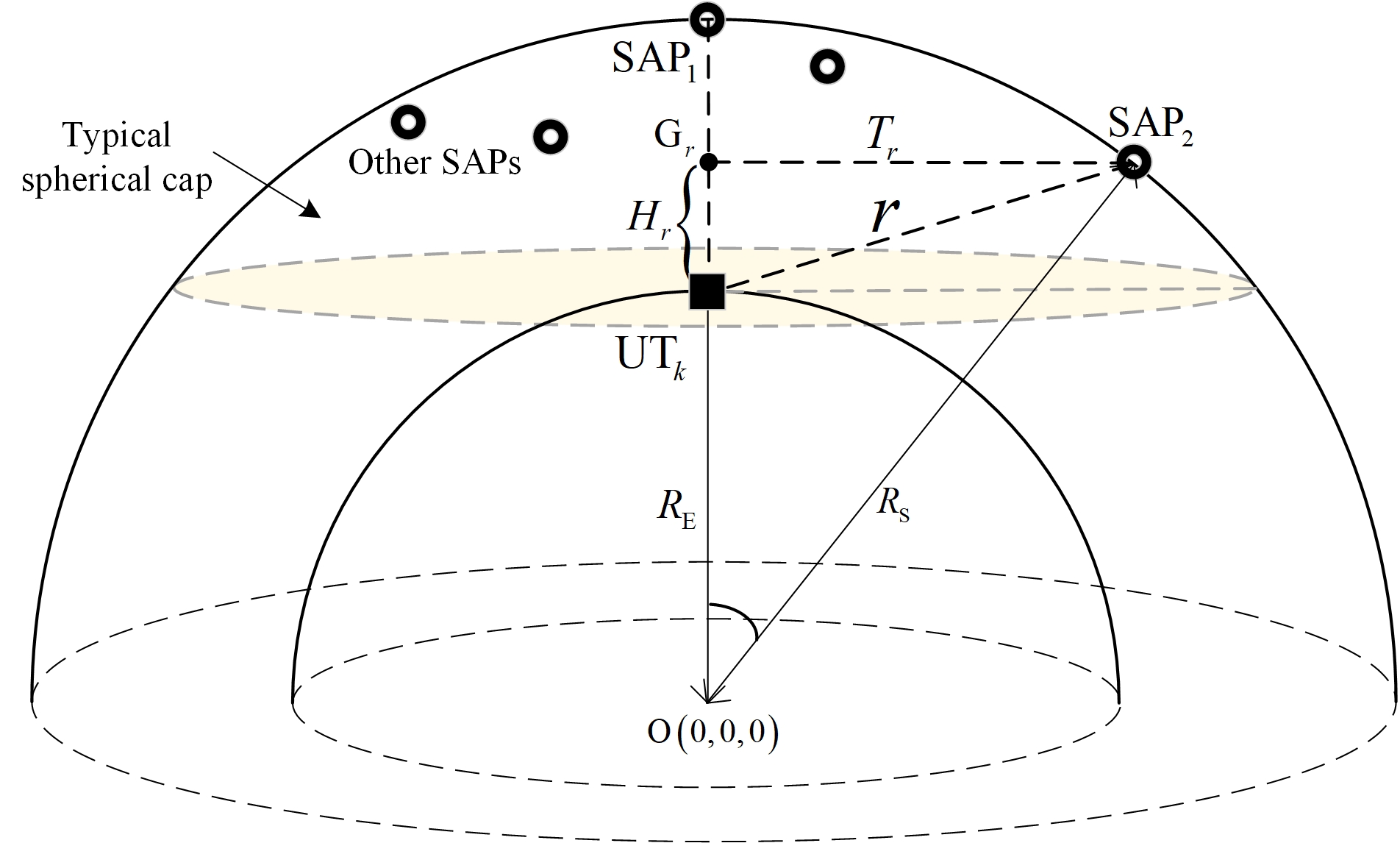
Related parameters in the stochastic geometry sketch of UTs and SAPs are labeled in Fig. 2. According to the 3GPP Technical Standard [34], each ground UT has a maximum service range for satellites. Thus, the typical UT has a dome angle from its position and corresponds to the shortest vertical distance from the UT. We denote the area marked in light yellow as a “service range” corresponding to . If an SAP is within the service range, that is, if its vertical distance from the UT is longer than , it is considered a service SAP. A cluster of SAPs within the service range is coordinated by the CS to serve the UT coherently.
Let the distance from the typical UT to any one of the service SAPs be . According to [1, Lemma 1], the cumulative distribution function (CDF) of is given in (9) at the bottom of the page,
| (9) |
where , and the corresponding PDF is given by
| (10) |
for , while , otherwise. Note that and are the minimum and maximum distances from the typical UT to a service SAP, respectively, and is the maximum distance from the typical UT to any SAP [15].
Next, the shortest vertical distance from service SAPs to the typical UT is given by [1, Lemma 2]
| (11) |
Then, the maximum distance from a service SAP to the typical UT is for , and for .
Finally, due to the change of , each SAP has a service area on the earth’s surface. The average number of UTs within this service area is written as [1, Lemma 3]
| (12) |
III-B Analytical Expressions
The coverage probability is determined by the signal-to-interference-plus-noise ratio (SINR) of the message received by a typical UT and a threshold . When the SINR is above the threshold , this UT can successfully decode the data. Following the expression for the signals received by the -th UT in (8), the corresponding SINR is
| (13) |
where , , .
Proposition 1.
The CCDF of the DSS received by the typical UT is given in (14) at the bottom of the next page, where .
| (14) | ||||
Proof.
Please see Appendix A. ∎
Proposition 2.
The average multi-user interference received by the typical UT is given by
| (15) | ||||
where is provided in (12), and the average inter-satellite interference received by the typical UT is given by
| (16) | ||||
Proof.
Please see Appendix B. ∎
Theorem 1.
The coverage probability on the Nakagami- fading channel is given in (17) at the bottom of the page, where , and are given in Proposition 2.
| (17) |
Proof.
Due to the characterization of CCDF, by inserting the right-hand side in the last step of (31), which includes the interference signal power in Proposition 2 and the noise power , into the CCDF of the desired signal part shown in (14) of Proposition 1, an approximate expression is obtained for the coverage probability of the CF-mMIMO SatCom network in (17) at the bottom of the page, which completes the proof. ∎
IV Performance Analysis under Non-Fading Channels
In this section, we derive the coverage probability in the scenario without fading in the CF-mMIMO LEO SatCom network. This scenario is applicable when the number of SAPs in a constellation is large enough [15], which is suitable for our studied network. Since UTs, such as airplanes, can be high in altitude in some cases, the direct propagation paths from multiple service SAPs are dominant, and the multi-path fading components are comparatively weaker than the former.
Similar to Theorem 1, we first calculate the CCDF of the DSS and then obtain the analytical results of the overall coverage probability.
Proposition 3.
The CCDF of the DSS received by the typical UT under non-fading propagation environments is given in (18) at the bottom of the next page.
| (18) | ||||
Proof.
Omitting the channel term, the coverage probability under non-fading propagation environments is represented as
| (19) | ||||
where the multi-user interference is , and the inter-satellite interference is . The DSS can be expressed as
| (20) | ||||
where we denote .
The Laplace transform of DSS is
| (21) | ||||
where .
Similar to (42)-(43), the CDF of can be derived as
| (22) | ||||
where . By inserting (21) into (22), the CDF of can be obtained as in (23) at the bottom of the next page.
| (23) |
Proposition 4.
The average multi-user interference received by the typical UT under non-fading channels is
| (24) | ||||
and the average inter-satellite interference received by the typical UT under non-fading channels is
| (25) |
Proof.
The average multi-user interference can be derived as
| (26) | ||||
where follows from the approximation for the derivation of interference signals from surrounding base stations in [35, 36]; in , is provided in (12), and the equation holds true because of the large-scale deployment of LEO satellites; is obtained according to the nature of expectation and using Campbell’s theorem.
Similarly, the average inter-satellite interference can be obtained by
| (27) | ||||
which completes the proof. ∎
Theorem 2.
The coverage probability of the typical UT under non-fading propagation environments is given by (28) at the bottom of the next page, where , and are provided in Proposition 4.
| (28) |
Proof.
Using the mutual relationship between CDF and CCDF, and inserting the average interference in Proposition 4 into the CCDF expression of DSS in (23) of Proposition 3, an approximate expression for the coverage probability of typical UT is obtained in (28) at the bottom of the next page, which completes the proof. ∎
V Simulation Results and Discussions
In this section, we quantitatively investigate the downlink performance of the CF-mMIMO satellite network with respect to essential parameters, including dome angle, orbital altitude and number of SAPs, Nakagami fading parameter , etc. In particular, we also study the coverage probability under non-fading propagation environments considering the weak multi-path components over the long communication distances between SAPs and UTs. The analytical results are provided based on the statistical properties and expressions in Sections II, III and IV. We use Monte Carlo simulations to obtain the DSS, coverage probability, capacity, and other tentative indexes for numerical and analytical verification. The system parameters are summarized in Table I according to [6, 15, 26, 34], and other parameters are based on different scenario settings.
| Parameter | Value |
|---|---|
| Radius of Earth | 6371.393 km |
| Density of SAPs | /km2 |
| Density of UTs | /km2 |
| Carrier frequency | GHz |
| Transmit power of downlink data | dBm |
| Transmit power of pilot symbol | dBm |
| Noise power | dBm |
| SAP antenna gain | dBi |
| UT antenna gain | dBi |
| Nakagami parameter | 2.0 |
| Path-loss exponent |
To validate the suitability of the PPP model for the studied network, we first compare the coverage probability under the PPP model, random-initial-state Starlink constellation, and fixed-initial-state Starlink constellation, with an inclination angle and an example orbital altitude of km [18, 37]. Fig. 3 shows that the coverage gap between the PPP model and the fixed-initial-state Starlink constellation is more significant than that between the PPP model and the random-initial-state Starlink constellation. This indicates that the PPP model can fit the actual constellation well with the random-initial-state Starlink constellation model. As the actual constellation is close to the random-initial-state Starlink constellation, it is reasonable to use the PPP model for approximation. Moreover, it is assumed that the distribution of SAPs is not correlated with the PPP for the derivation of analytical results.
To understand how well the analytical DSS matches its simulation counterparts, we compare its CCDF with that under perfect and imperfect CSI in Fig. 4. The CCDF of DSS with imperfect CSI depends on the number of pilots during the uplink training stage. Specifically, when , an apparent gap can be witnessed between the CCDF of DSS under imperfect CSI and that under perfect CSI. However, the gap reduces as more pilots are utilized, e.g., , . We can see that the increase in the pilots’ number gives rise to a more accurate DSS, approximating one under perfect CSI. It can also be seen that the analytical DSS matches the simulation DSS well under perfect CSI. Thus, it is reasonable to use this analytical expression for further investigation.
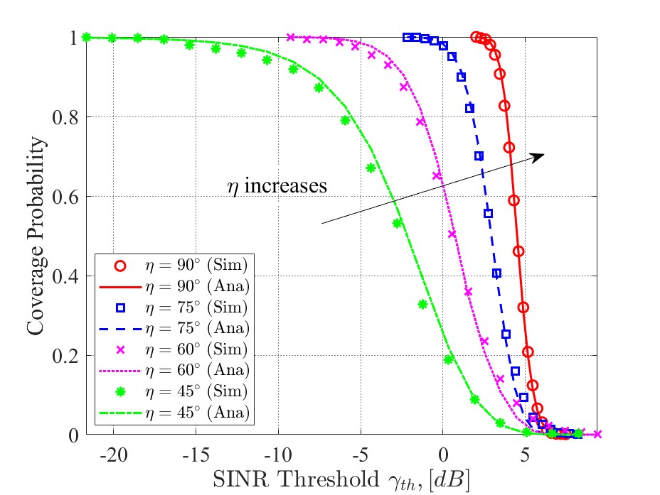
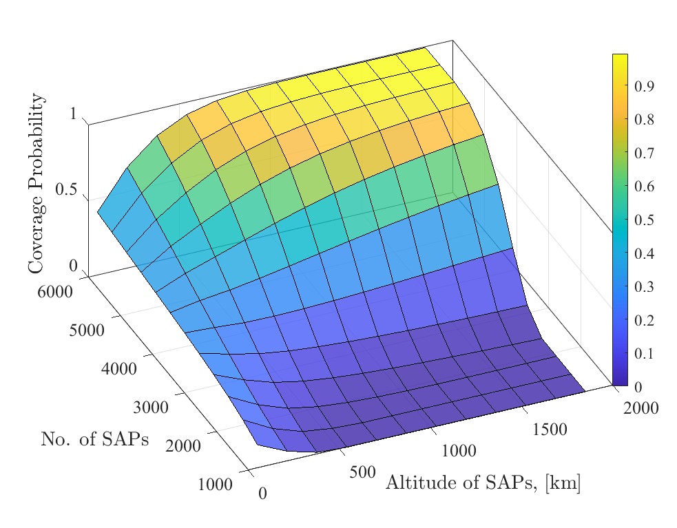
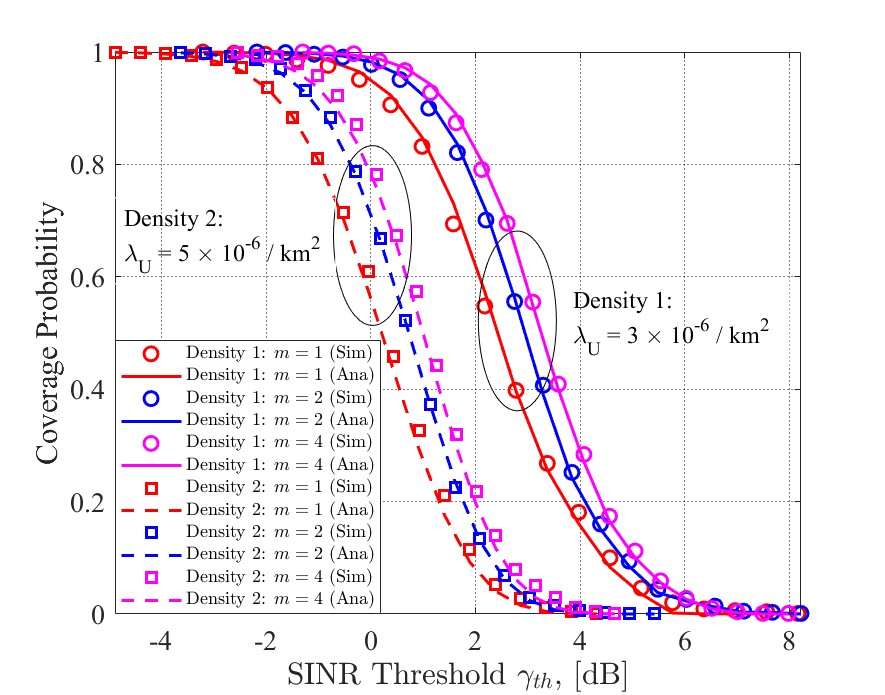
Fig. 5 compares the coverage probability under different UT densities and Nakagami fading parameters . It is shown that the analytical results from Theorem 1 match closely with simulations in different values of . Specifically, when the UT density /km2, for thresholds between around dB and dB, the coverage probability of case is higher than that of case , followed by that of case . The gap between case and first increases to about when dB before decreasing to 0 after dB. A similar but less obvious trend can also be seen between the cases of and , and for the cases when /km2.
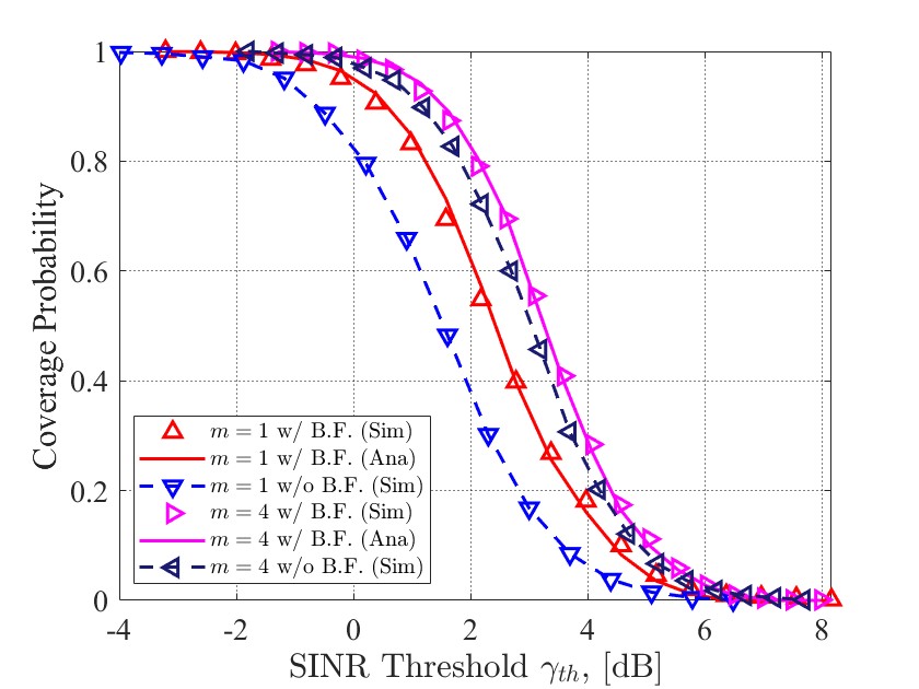
Fig. 6 compares the coverage performance under the Nakagami- fading channel with beamforming and without beamforming. For both beamforming and non-beamforming pairs under and , a clear gap can be witnessed: under the same SINR threshold requirements, fading channels with beamforming bring higher coverage than their counterparts without beamforming. Thus, beamforming still counts in terms of providing better coverage for the CF-mMIMO SatCom network.
Then, we explore the impacts of the service range brought by the dome angle . Fig. 7 demonstrates the coverage probability for different values of ranging from to . We notice that the increase of brings higher coverage when the SINR threshold is between dB and dB. However, all coverage probability values converge to at about dB. This is because a larger service range incorporates more satellites into the CF-mMIMO SatCom network, although multi-user interference exists. Thus, a UT with a larger service range will enjoy higher coverage.
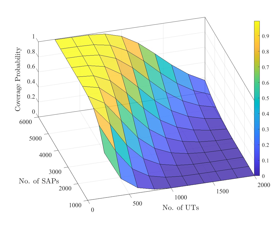
Next, dual influences of orbital altitude and number of SAPs are shown in Fig. 8 in a three-dimensional (3D) view. We observe that for a fixed altitude in the given range, increasing the number of SAPs always brings higher coverage. However, coverage declines as the altitude increases when the number of SAPs is smaller than approximately , whereas it increases with the rise of altitude when the number of SAPs is larger than . It shows that conditioned on dB, when the total number of SAPs is relatively small, the increase in the number of SAPs fails to compensate for the desired signal reduction resulting from extended propagation distances, which is a consequence of increased altitude. In addition, we study the effect of the number of UTs and the number of SAPs on the coverage probability. Fig. 9 shows that fewer UTs and more SAPs are preferred for higher coverage. This accords with the facts in terrestrial CF-mMIMO systems, where the performance of an individual UT can experience a substantial enhancement when a large number of APs are serving a smaller number of UTs.
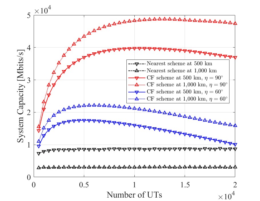
Fig. 10 compares the ergodic system capacity of the CF-mMIMO SatCom network, i.e., CF scheme, with that of the satellite service scheme in [15], where a UT is only served by the nearest satellite. By considering the channel estimation overhead and both uplink and downlink durations, the system capacity of the CF scheme is defined as
| (29) | ||||
and the system capacity of the nearest-satellite-service scheme is given by
| (30) |
where denotes the total number of UTs on the earth’s surface, , and . In the nearest-satellite-service scheme, for both altitudes of km and km, a slight increase in system capacity can be observed when the number of UTs grows from to before reaching a plateau. The system capacity at km is greater than that at km. However, different trends are seen for the CF scheme. The system capacity at km is greater than that at km, for both and . This is because a higher altitude at a fixed incorporates more SAPs into the CF-mMIMO SatCom network. Therefore, a larger dome angle and a higher altitude improve the system capacity. Moreover, there is an optimal number of UTs for each at a certain altitude, and the optimal number rises with an increase in or altitude. The above schemes are also compared regarding per-user capacity in Fig. 11, which is defined as and for the CF scheme [19] and nearest-satellite-service scheme, respectively. A decreasing trend is witnessed for all these cases. Specifically, the CF scheme with and altitude km has the highest per-user capacity for all numbers of UTs. All CF schemes offer higher per-user capacity than the nearest-satellite-service scheme does. Note that when there are UTs in total, both the system capacity and the per-user capacity in the CF scheme with and altitude km approach those of the nearest satellite service scheme. This indicates that the high-performance gain of the CF-mMIMO SatCom network may vanish with the growing number of UTs.
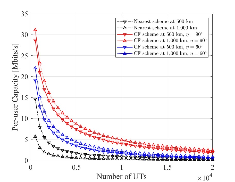
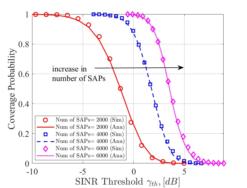
Fig. 12 compares the coverage probability against the SINR threshold for different orbital altitudes of SAPs under the non-fading scenario. With an increase in the number of SAPs, the coverage probability becomes higher under the given SINR threshold. This is in line with the findings under the previous with-fading scenarios, and it shows that the analytical expressions match well with the simulation results.
VI Conclusions
In this paper, we analyzed the CF-mMIMO LEO SatCom network in terms of coverage and capacity from a system-level perspective. Using the tools from stochastic geometry, we modeled the satellite network in two SPPPs and derived the coverage probability in both fading and non-fading scenarios, with significant network parameters such as Nakgami fading parameter, path-loss factor, orbital altitude, number of SAPs, and service range brought by the dome angle. The Laplace transform and relevant numerical approximation methods are involved in analyzing the desired and interference signals. Based on these numerical and analytical results obtained, we find that beamforming plays an essential role in network performance, and the direct distance-related propagation path dominates the quality of signals. Increasing the service range, orbital altitude, and number of SAPs is shown to improve coverage performance. Furthermore, while there is an optimal number of UTs to maximize the system capacity, the capacity for each individual UT declines as the number of UTs increases. Although additional SAPs can be accommodated by raising their orbital altitudes, the corresponding increase in costs and communication latency should be considered in the real-world deployment of satellite networks.
Appendix A Proof of Proposition 1
By inserting , the coverage probability of the typical UT is represented as
| (31) | ||||
where , . We consider the perfect channel estimation in deriving an upper bound of the DSS.
To derive the coverage probability, we need to compute both the distribution of DSS and the average interference power. First, the distribution of is calculated as follows.
| (32) | ||||
Denote . The PDF of is obtained from the Laplace transform of , which is
| (33) | ||||
where
| (34) |
The Laplace transform of is
| (35) | ||||
where is first computed as follows. As the norm of channel ,
whose PDF is , we have
| (36) | ||||
where follows from a combinations of exponentials of more complicated arguments and powers in [38, Equation 3.462.1], is written as (37) at the bottom of the next page, and follows from the parabolic cylinder function in [38, Equation 9.240.1].
| (37) |
Then, by inserting (36) back into (35), the Laplace transform of the desired signal power can be further written as
| (38) | ||||
where follows from the probability generating function (PGFL) of the PPP.
To illustrate the relationship between the satellite-terrestrial distance and other parameters on two spheres, Fig. 13 is provided, where the previous distance symbol is re-represented by based on the SAP-to-UT distance . The area of the typical spherical cap is . Let the distance from a randomly-selected SAP on the sphere to the typical UT be . In Triangle by SAP2, point and original point O, the height of can be derived by using Pythagorean theorem , and in Triangle formed by SAP2, point and UTk, distance can be written as . By combining the above two formulas, the expression for on is given by . Then, the typical spherical cap can be further represented as
| (39) | ||||
The derivation of on is
| (40) |
By inserting (40) into (38), we can further derive as in (41), which is at the bottom of the page.
| (41) | ||||
| (42) | ||||
To derive the CDF of , we have an integral over its PDF and adopt the inverse Laplace transform method for the PDF [39], where it can be calculated by Bromwich contour integral method. Moreover, it can also be estimated using summation forms of integrals with a controllable error [40]. We derive the CDF of , as
| (43) | ||||
where holds true according to the definition of inverse Laplace transform, and is obtained based on in probability theory. Following [41], (43) can be approximated by a finite sum which is expressed as in (42) at the bottom of the page, where , and is obtained in (41). , , and are positive parameters used to adjust the accuracy of approximation. We also let for and for .
Appendix B Proof of Proposition 2
The average multi-user interference can be represented as
| (44) | ||||
where is approximated due to the nature of normalization of , follows an approximation by summing interference from required base stations as in [35], comes from the average number of UTs in the coverage of an SAP, and in , the integral is obtained due to the nature of expectation. Similarly, the inter-satellite interference can be derived as
| (45) | ||||
Finally, closed-form expressions are obtained by inserting (40) and using Campbell’s theorem, which completes the proof.
References
- [1] X. Li and B. Shang, “An analytical model for coordinated multi-satellite joint transmission system,” in Proc. Int. Conf. Ubiquitous Commun. (Ucom), Jul. 2024, pp. 169–173.
- [2] K.-X. Li, L. You, J. Wang, X. Gao, C. G. Tsinos, S. Chatzinotas, and B. Ottersten, “Downlink transmit design for massive mimo leo satellite communications,” IEEE Trans. Commun., vol. 70, no. 2, pp. 1014–1028, Nov. 2021.
- [3] L. You, K.-X. Li, J. Wang, X. Gao, X.-G. Xia, and B. Ottersten, “Massive mimo transmission for leo satellite communications,” IEEE J. Sel. Areas Commun., vol. 38, no. 8, pp. 1851–1865, Jun. 2020.
- [4] L. You, X. Qiang, K.-X. Li, C. G. Tsinos, W. Wang, X. Gao, and B. Ottersten, “Hybrid analog/digital precoding for downlink massive mimo leo satellite communications,” IEEE Trans. Wireless Commun., vol. 21, no. 8, pp. 5962–5976, Jan. 2022.
- [5] M. Á. Vázquez, A. Perez-Neira, D. Christopoulos, S. Chatzinotas, B. Ottersten, P.-D. Arapoglou, A. Ginesi, and G. Taricco, “Precoding in multibeam satellite communications: Present and future challenges,” IEEE Wireless Commun., vol. 23, no. 6, pp. 88–95, Dec. 2016.
- [6] B. Shang, X. Li, Z. Li, J. Ma, X. Chu, and P. Fan, “Multi-connectivity between terrestrial and non-terrestrial mimo systems,” IEEE Open J. Commun. Soc., vol. 5, pp. 3245–3262, May 2024.
- [7] D. Goto, H. Shibayama, F. Yamashita, and T. Yamazato, “Leo-mimo satellite systems for high capacity transmission,” in Proc. IEEE Global Commun. Conf. (GLOBECOM). IEEE, Dec. 2018, pp. 1–6.
- [8] L. Lu, G. Y. Li, A. L. Swindlehurst, A. Ashikhmin, and R. Zhang, “An overview of massive mimo: Benefits and challenges,” IEEE J. Sel. Topics Signal Process., vol. 8, no. 5, pp. 742–758, Apr. 2014.
- [9] J. Xu, M. A. Kishk, and M.-S. Alouini, “Space-air-ground-sea integrated networks: Modeling and coverage analysis,” IEEE Trans. Wireless Commun., vol. 22, no. 9, pp. 6298–6313, Feb. 2023.
- [10] W. Lu and M. Di Renzo, “Stochastic geometry modeling and system-level analysis & optimization of relay-aided downlink cellular networks,” IEEE Trans. Commun., vol. 63, no. 11, pp. 4063–4085, Sep. 2015.
- [11] S. Fang, G. Chen, X. Xu, S. Han, and J. Tang, “Millimeter-wave coordinated beamforming enabled cooperative network: a stochastic geometry approach,” IEEE Trans. Commun., vol. 69, no. 2, pp. 1068–1079, Nov. 2020.
- [12] A. Talgat, M. A. Kishk, and M.-S. Alouini, “Stochastic geometry-based analysis of leo satellite communication systems,” IEEE Commun. Lett., vol. 25, no. 8, pp. 2458–2462, Oct. 2020.
- [13] D. Kim, J. Park, and N. Lee, “Coverage analysis of dynamic coordinated beamforming for leo satellite downlink networks,” IEEE Trans. Wireless Commun., vol. 23, no. 9, Apr. 2024.
- [14] N. Okati, T. Riihonen, D. Korpi, I. Angervuori, and R. Wichman, “Downlink coverage and rate analysis of low earth orbit satellite constellations using stochastic geometry,” IEEE Trans. Commun., vol. 68, no. 8, pp. 5120–5134, Apr. 2020.
- [15] J. Park, J. Choi, and N. Lee, “A tractable approach to coverage analysis in downlink satellite networks,” IEEE Trans. Wireless Commun., vol. 22, no. 2, pp. 793–807, Aug. 2022.
- [16] R. Deng, B. Di, H. Zhang, L. Kuang, and L. Song, “Ultra-dense leo satellite constellations: How many leo satellites do we need?” IEEE Trans. Wireless Commun., vol. 20, no. 8, pp. 4843–4857, Mar. 2021.
- [17] H. Jia, Z. Ni, C. Jiang, L. Kuang, and J. Lu, “Uplink interference and performance analysis for megasatellite constellation,” IEEE Internet Things J., vol. 9, no. 6, pp. 4318–4329, Aug. 2022.
- [18] H. Jia, C. Jiang, L. Kuang, and J. Lu, “An analytic approach for modeling uplink performance of mega constellations,” IEEE Trans. Veh. Technol., vol. 72, no. 2, pp. 2258–2268, Feb. 2023.
- [19] H. Q. Ngo, A. Ashikhmin, H. Yang, E. G. Larsson, and T. L. Marzetta, “Cell-free massive mimo versus small cells,” IEEE Trans. Wireless Commun., vol. 16, no. 3, pp. 1834–1850, Jan. 2017.
- [20] T. Zhao, X. Chen, Q. Sun, and J. Zhang, “Energy-efficient federated learning over cell-free iot networks: Modeling and optimization,” IEEE Internet Things J., vol. 10, no. 19, pp. 17 436–17 449, May 2023.
- [21] Q. Sun, X. Ji, Z. Wang, X. Chen, Y. Yang, J. Zhang, and K.-K. Wong, “Uplink performance of hardware-impaired cell-free massive mimo with multi-antenna users and superimposed pilots,” IEEE Trans. Commun., vol. 71, no. 11, pp. 6711–6726, Aug. 2023.
- [22] C. Liu, W. Feng, Y. Chen, C.-X. Wang, and N. Ge, “Cell-free satellite-uav networks for 6g wide-area internet of things,” IEEE J. Sel Areas Commun., vol. 39, no. 4, pp. 1116–1131, Aug. 2020.
- [23] J. Li, L. Chen, P. Zhu, D. Wang, and X. You, “Satellite-assisted cell-free massive mimo systems with multi-group multicast,” Sensors, vol. 21, no. 18, p. 6222, Sep. 2021.
- [24] M. Y. Abdelsadek, H. Yanikomeroglu, and G. K. Kurt, “Future ultra-dense leo satellite networks: A cell-free massive mimo approach,” in Proc. IEEE Int. Conf. Commun. Workshops (ICC Workshops). IEEE, Jun. 2021, pp. 1–6.
- [25] M. Y. Abdelsadek, G. K. Kurt, and H. Yanikomeroglu, “Distributed massive mimo for leo satellite networks,” IEEE Open J. Commun. Soc., vol. 3, pp. 2162–2177, Nov. 2022.
- [26] M. Y. Abdelsadek, G. Karabulut-Kurt, H. Yanikomeroglu, P. Hu, G. Lamontagne, and K. Ahmed, “Broadband connectivity for handheld devices via leo satellites: Is distributed massive mimo the answer?” IEEE Open J. Commun. Soc., vol. 4, pp. 713–726, Mar. 2023.
- [27] S. Yang, D. Wang, L. Liu, B. Wang, and C. Sun, “Distributed multiple leo satellites cooperative downlink power enhancement transmission scheme based on otfs,” in Proc. IEEE Int. Conf. Commun. Technol. (ICCT). IEEE, Feb. 2024, pp. 1208–1213.
- [28] Y. Omid, Z. M. Bakhsh, F. Kayhan, Y. Ma, F. Wang, and R. Tafazolli, “On capacity of handheld to multi-satellite communication,” in Proc. IEEE 34th Annu. Int. Symp. Pers., Indoor and Mobile Radio Commun. (PIMRC). IEEE, Oct. 2023, pp. 1–5.
- [29] Y. Omid, Z. M. Bakhsh, F. Kayhan, Y. Ma, and R. Tafazolli, “Space mimo: Direct unmodified handheld to multi-satellite communication,” in Proc. IEEE Global Commun. Conf. (GLOBECOM). IEEE, Feb. 2024, pp. 1447–1452.
- [30] Y. Omid, S. Lambotharan, and M. Derakhshani, “Tackling delayed csi in a distributed multi-satellite mimo communication system,” arXiv:2406.06392. [Online]. Available: https://arxiv.org/abs/2406.06392, 2024.
- [31] K. Humadi, G. K. Kurt, and H. Yanikomeroglu, “Distributed massive mimo system with dynamic clustering in leo satellite networks,” arXiv:2404.06024. [Online]. Available: https://arxiv.org/abs/2404.06024, 2024.
- [32] B. Shang, X. Li, C. Li, and Z. Li, “Coverage in cooperative leo satellite networks,” J. Commun. Inf. Netw., vol. 8, no. 4, pp. 329–340, Dec. 2023.
- [33] R. Richter, I. Bergel, Y. Noam, and E. Zehavi, “Downlink cooperative mimo in leo satellites,” IEEE Access, vol. 8, pp. 213 866–213 881, Nov. 2020.
- [34] 3GPP, “Solutions for NR to support Non-Terrestrial Networks (NTN),” 3rd Generation Partnership Project (3GPP), Technical Report (TR) 38.821, 06 2021, version 16.1.0.
- [35] G. Nigam, P. Minero, and M. Haenggi, “Coordinated multipoint joint transmission in heterogeneous networks,” IEEE Trans. Commun., vol. 62, no. 11, pp. 4134–4146, Oct. 2014.
- [36] D. Maamari, N. Devroye, and D. Tuninetti, “Coverage in mmwave cellular networks with base station co-operation,” IEEE Trans. Wireless Commun., vol. 15, no. 4, pp. 2981–2994, Jan. 2016.
- [37] B. Al Homssi and A. Al-Hourani, “Modeling uplink coverage performance in hybrid satellite-terrestrial networks,” IEEE Commun. Lett., vol. 25, no. 10, pp. 3239–3243, Oct. 2021.
- [38] D. Zwillinger and A. Jeffrey, Table of integrals, series, and products. Elsevier, 2007.
- [39] B. Shang, L. Zhao, and K.-C. Chen, “Enabling device-to-device communications in lte-unlicensed spectrum,” in Proc. IEEE Int. Conf. Commun. (ICC). IEEE, Jul. 2017, pp. 1–6.
- [40] A. M. Cohen, Numerical methods for Laplace transform inversion. Springer Science & Business Media, 2007, vol. 5.
- [41] X. Zhou, J. Guo, S. Durrani, and M. Di Renzo, “Power beacon-assisted millimeter wave ad hoc networks,” IEEE Trans. Commun., vol. 66, no. 2, pp. 830–844, Oct. 2017.