Downlink Extrapolation for FDD Multiple Antenna Systems Through Neural Network Using Extracted Uplink Path Gains

We consider a scenario that the NN at the BS is trained with the UL and DL CSI from a given path where MSs travel and conduct the DL extrapolation for a new MS entering the same path. The DL extrapolation is possible as long as the UL and DL experience the channel reciprocity in FDD. Figs. 3-(a) and (b) are the snapshots of channels in different carrier frequencies, which are generated by Wireless InSite, a commercial ray-tracing simulator [24]. As shown in the figures, the traces of UL signal, with 2.14 GHz carrier frequency, and DL signal, with 1.95 GHz carrier frequency, are almost identical even with the guard band between the two.

To exploit the NN for DL extrapolation, the BS should collect the CSI data from MSs moving on the same path. A typical scenario of an urban communication system is depicted in Fig. 2. Since urban roads restrict the course of MSs as shown in the figure, the tracks of MSs on a given path can be assured to be nearly identical. We exploit QuaDRiGa [23] to obtain samples of the UL and DL channels since it considers complicated physics including mobility for channel emulation. The channel samples obtained from QuaDRiGa does not have any idealistic feature, e.g., perfect directional reciprocity between the UL and DL channels. This is quite different from previous works where channel samples are obtained based on analytical channel models [15, 16, 18, 25, 19, 20, 21, 22, 26].

QuaDRiGa periodically generates channel snapshots for each MS moving on a given path. The MS sample set is a set of channel snapshots of one MS along the given path. The environment geometry on a given path, e.g., nearby buildings, is maintained for a long time. Therefore, the MSs on the same path would experience high spatial correlation. However, specific signal paths may vary temporarily due to large dynamic objects like moving trucks. Taking this situation into an account, for each MS sample set, we fix several clusters to reflect the static environments and randomly change a few clusters to reflect the dynamic objects. The UL and DL channels for each MS have the same clusters to maintain their geometrical reciprocity.

Remark 1: Even with the trained NN, it takes a time for the BS to conduct the DL extrapolation. When the BS estimates the UL CSI at $t_{0}$, it needs to infer the DL CSI at $t_{0}+d$ where $d$ is the processing delay for the DL extrapolation. Thus, we generate UL and DL channels to keep their time interval $d$.

Remark 2: To implement the DL extrapolation using the NN, the BS has to collect the UL and DL CSI as training data sets. In the conventional limited feedback for FDD, the BS can only access to quantized DL CSI. Still, we believe it is possible to train the NN with high resolution DL CSI once services providers obtain the required data sets offline since the NN training is not a real-time process. Although the exact timestamps of UL and DL CSI data may be different, the timing difference can be adjusted before the training process since the training is performed after stacking the data. After the services providers train the NN using collected UL and DL CSI, the BS only needs to operate the DL extrapolation function in real-time using the trained NN stored in its memory.

The channel generated by QuaDRiGa can be approximated as

which consists of $L$ paths and $P$ subpaths per path where $L$ represents the number of clusters in our case. In (1), $f_{\mathrm{c}}$ is the carrier frequency, $\alpha_{\ell,p}(f_{\mathrm{c}})$ is the path gain, $\tau_{\ell}$ is the delay, and $\theta_{\ell,p}$ is the AoD. We assume the path gains and AoDs are subpath dependent while all subpaths from the same cluster experience the same delay. The $N_{\mathrm{BS}}\times 1$ vector ${\mathbf{a}}(\theta_{\ell,p})$ is the array response of the signal incident at $\theta_{\ell,p}$, where $N_{\mathrm{BS}}$ is the number of BS antennas.

The channel due to the $\ell$-th cluster is given as

The channel coefficient of the $\ell$-th cluster $\boldsymbol{\mathfrak{h}}_{\ell}(f_{c})$ consists of $P$ subpath components; $\boldsymbol{\mathfrak{h}}_{\ell}(f_{c})=\sum_{p=1}^{P}\alpha_{\ell,p}(f_{c}){\mathbf{a}}(\theta_{\ell,p})$. While the path gains are frequency dependent components, we assume the delays and AoDs are frequency independent components as in [13], i.e., the UL and DL channels experience the same delays and AoDs due to the same geometry.

The channel in (1) can be transformed into the frequency domain. The $k$-th subcarrier of the orthogonal frequency division multiplexing (OFDM) channel is obtained as [13]

where $f_{\mathrm{s}}$ is the total bandwidth, and $K$ is the total number of subcarriers. We use the underline to denote variables in the frequency domain throughout the paper. By concatenating all subcarriers, we have the $N_{\mathrm{BS}}\times K$ OFDM channel matrix $\underline{{\mathbf{H}}}(f_{c})=[\underline{{\mathbf{h}}}_{1}(f_{c})\cdots\underline{{\mathbf{h}}}_{K}(f_{c})]$. The OFDM channel matrix $\underline{{\mathbf{H}}}(f_{c})$ can be rewritten as

where ${\mathbf{p}}(\tau_{\ell})=[e^{-j2\pi f_{s}\tau_{\ell}\frac{1}{K}},e^{-j2\pi f_{s}\tau_{\ell}\frac{2}{K}},\dots,e^{-j2\pi f_{s}\tau_{\ell}}]^{\mathrm{T}}$. Each element of ${\mathbf{p}}(\tau_{\ell})$ matches with the subcarrier of the OFDM channel.

In the DL training, the MS estimates the DL channel and feeds back the acquired information to the BS. First, the BS transmits the pilot symbol ${\mathbf{s}}_{\mathrm{dl}}(t)$ to the MS. The received signal at the MS in the time domain is written as

where ${\mathbf{s}}_{\mathrm{dl},j}(t)$ is the $j$-th pilot symbol with $j\in\{1,\dots,J\}$, generally, $J\geq N_{\mathrm{BS}}$. The additive white Gaussian noise $w_{\mathrm{dl},j}(t)$ has zero mean with variance $N_{0}$. To estimate the DL CSI, the MS first stacks the $J$ received pilot signals as

where ${\mathbf{y}}(t,f_{\mathrm{dl}})=[y_{1}(t,f_{\mathrm{dl}}),\dots,y_{J}(t,f_{\mathrm{dl}})]^{\mathrm{T}}$, ${\mathbf{S}}_{\mathrm{dl}}(t)=[{\mathbf{s}}_{\mathrm{dl},1}(t),$ $\dots,{\mathbf{s}}_{\mathrm{dl},J}(t)]$, and ${\mathbf{w}}_{\mathrm{dl}}(t)=[w_{\mathrm{dl},1}(t),\dots,w_{\mathrm{dl},J}(t)]^{\mathrm{T}}$. Using the transformation in (II-B), the received signal in the frequency domain is represented as

Using the least square (LS) estimator based on the known $\underline{{\mathbf{S}}}_{\mathrm{dl},k}$, the estimated DL CSI is given as

Repeating the above process for all subcarriers, the DL OFDM channel $\hat{\underline{{\mathbf{H}}}}(f_{\mathrm{dl}})$ can be obtained.

The DL training needs to be performed for every coherence time interval, and the training overhead normally increases as the number of antennas at the BS increases. Considering the training overhead, the effective spectral efficiency is given as

In (9), $\mathfrak{R}$ is the spectral efficiency, which is defined as [3]

where $\rho$ is the signal-to-noise ratio (SNR). We assume the perfect UL feedback in (10) to check the upper bound of the DL training-based transmission. The coherence time interval decreases as the speed of the MS increases, so the conventional DL-training-based approach is not appropriate for high mobility scenarios in FDD.

The purpose of using the NN is to estimate the DL CSI directly from the UL CSI measured at the BS without having any explicit downlink training. More precisely, the previous works in [15, 16] used the UL OFDM channel $\underline{{\mathbf{H}}}(f_{\mathrm{ul}})$ as an input and the DL OFDM channel $\underline{{\mathbf{H}}}(f_{\mathrm{dl}})$ as an output to train the NN, i.e.,

where ${\mathcal{Q}}_{\mathrm{CH}}(\cdot)$ denotes the function of NN-based DL extrapolation. We will denote this approach as “CH-learning” in the remaining of paper. Since the numbers of antennas at the BS and subcarriers in OFDM could be quite large, the CH-learning may suffer from heavy computational complexity.

As explained in Remark 1, the DL extrapolation technique estimates the DL CSI at time $t_{0}+d$ using the UL CSI at time $t_{0}$. To simplify the notation, we intentionally neglect the delay $d$ in the following discussions.

In our proposed NN-based DL extrapolation, the DL channel can be reconstructed as

where the delay $\tilde{\tau}_{\ell}$ and AoD $\tilde{\theta}_{\ell,p}$ are the extracted parameters from the UL CSI, which will be explained in Sections IV-C and IV-D. The DL path gain $\check{\alpha}_{\ell,p}(f_{\mathrm{dl}})$ is the parameter predicted from the extracted UL path gain $\tilde{\alpha}_{\ell,p}(f_{\mathrm{ul}})$ using the NN, i.e.,

The function ${\mathcal{Q}}_{\mathrm{PG}}(\cdot)$ in (13) represents the network of the PG-learning. The detailed network structures of the PG-learning are explained in Section V-C.

We use the tilde $\tilde{a}$ to denote extracted parameters from the UL CSI and the check $\check{a}$ to represent predicted parameters using the NN throughout the paper. In (12), $R$ is the number of subpaths used for the channel reconstruction, $R\leq Q$, and $Q$ in (13) is the number of subpaths used for the learning, $Q\leq P$. The effects of $R$ and $Q$ are explained in Sections V-C and VI-A. Using (II-B), the reconstructed DL channel in the time domain in (12) can be converted to an OFDM channel.

The BS obtains the UL CSI through the UL training. When the MS transmits a pilot symbol $s_{\mathrm{ul}}(t)$ to the BS, the received signal at the BS in the time domain is written as

The $N_{\mathrm{BS}}\times 1$ vector ${\mathbf{w}}_{\mathrm{ul}}(t)$ is an additive white Gaussian noise with zero mean and variance $N_{0}{\mathbf{I}}$. After the transformation, the received signal at the $k$-th subcarrier can be obtained as

where the pilot symbol at the $k$-th subcarrier is $\underline{s}_{\mathrm{ul},k}={\mathcal{F}}_{k}\{s_{\mathrm{ul}}(t)\}$. The power of the transmitted symbol is constrained to $|\underline{s}_{\mathrm{ul},k}|^{2}\leq P_{\mathrm{ul}}$ for all $k$. The $N_{\mathrm{BS}}\times 1$ noise vector $\underline{{\mathbf{w}}}_{\mathrm{ul},k}=$ ${\mathcal{F}}_{k}\{{\mathbf{w}}_{\mathrm{ul}}(t)\}$ still maintains the same mean and variance as in the time domain case. For the known symbol $s_{\mathrm{ul}}(t)$, the BS estimates the UL channel using the LS estimator

where $\underline{{\mathbf{Y}}}(f_{\mathrm{ul}})=[\underline{{\mathbf{y}}}_{1}(f_{\mathrm{ul}})\cdots\underline{{\mathbf{y}}}_{K}(f_{\mathrm{ul}})]$, $\underline{{\mathbf{S}}}_{\mathrm{ul}}=\mathop{\mathrm{diag}}[\underline{s}_{\mathrm{ul},1},$ $\dots,\underline{s}_{\mathrm{ul},K}]$, and $\underline{{\mathbf{W}}}_{\mathrm{ul}}=[\underline{{\mathbf{w}}}_{\mathrm{ul},1}\cdots\underline{{\mathbf{w}}}_{\mathrm{ul},K}]$.

If the BS can access the time domain CSI, it is possible to directly obtain the noise corrupted $\ell$-th channel coefficient $\hat{\boldsymbol{\mathfrak{h}}}_{\ell}(f_{\mathrm{ul}})$ and delay $\hat{\tau}_{\ell}$ by observing impulses on the signal. If the BS only can access the OFDM channel $\hat{\underline{{\mathbf{H}}}}(f_{\mathrm{ul}})$, however, the BS has to figure out $\boldsymbol{\mathfrak{h}}_{\ell}(f_{\mathrm{ul}})$ and $\tau_{\ell}$. We consider two cases: 1) tPG-learning: the case when the BS can directly access the time domain signals, and 2) fPG-learning: the case when the BS only can access the frequency domain signals, which are elaborated in the following subsections.

In the tPG-learning, since the BS already has the estimated delay $\hat{\tau}_{\ell}$ and channel coefficient $\hat{\boldsymbol{\mathfrak{h}}}_{\ell}(f_{\mathrm{ul}})$, the BS only has to extract the AoDs and path gains.

Algorithm 1 shows how to extract the AoDs and path gains for the tPG-learning. In the beginning of the algorithm, the estimated channel coefficient $\hat{\boldsymbol{\mathfrak{h}}}_{\ell}(f_{\mathrm{ul}})$ is set to be ${\mathbf{h}}_{\ell}^{(0)}=\hat{\boldsymbol{\mathfrak{h}}}_{\ell}(f_{\mathrm{ul}})$. The AoD of the first subpath can be extracted as

After finding the AoD of the first subpath $\tilde{\theta}_{\ell,1}$ , the path gain $\tilde{\alpha}_{\ell,1}(f_{\mathrm{ul}})$ corresponding to $\tilde{\theta}_{\ell,1}$ can be obtained as

To find the parameters of other subpaths accurately, following a similar concept in [27], the effect of the dominant subpath could be cancelled by projecting ${\mathbf{h}}_{\ell}^{(0)}$ to the nullspace of ${\mathbf{a}}(\tilde{\theta}_{\ell,1})$.

where $\boldsymbol{{\mathcal{P}}}_{{\mathbf{a}}(\tilde{\theta}_{\ell,1})}^{\perp}$ is the projection matrix to the nullspace of ${\mathbf{a}}(\tilde{\theta}_{\ell,1})$, defined as

As replacing ${\mathbf{h}}_{\ell}^{(0)}$ with ${\mathbf{h}}_{\ell}^{(1)}$ and repeating the same process,the parameters of second subpath; $\tilde{\theta}_{\ell,2}$ and $\tilde{\alpha}_{\ell,2}(f_{\mathrm{ul}})$, can be found. All the parameters constituting $\hat{\boldsymbol{\mathfrak{h}}}_{\ell}(f_{\mathrm{ul}})$ can be inferred through $P$ iterations.

In the fPG-learning, since the time domain CSI is not available, the BS should first estimate the delays and channel coefficients before extracting the AoDs and path gains, as detailed in Algorithm 2. Similar to Algorithm 1, the delay $\tau_{\ell}$ can be obtained through the inner product maximization as in (24). After extracting $\tau_{\ell}$, projecting the estimated UL OFDM channel $\hat{\underline{{\mathbf{H}}}}(f_{\mathrm{ul}})$ to ${\mathbf{p}}(\tilde{\tau}_{\ell})$ gives the channel coefficient $\bar{\boldsymbol{\mathfrak{h}}}_{\ell}(f_{\mathrm{ul}})$ in (25). Since all channel coefficients $\boldsymbol{\mathfrak{h}}_{\ell}(f_{\mathrm{ul}})$ are composed of the AoDs $\theta_{\ell,p}$ and path gains $\alpha_{\ell,p}(f_{\mathrm{ul}})$, they should be in the form of $\boldsymbol{\mathfrak{h}}_{\ell}(f_{c})=\sum_{p=1}^{P}\alpha_{\ell,p}(f_{c}){\mathbf{a}}(\theta_{\ell,p})$. The channel coefficient $\bar{\boldsymbol{\mathfrak{h}}}_{1}(f_{c})$ obtained in (25), however, may not follow such from since $\bar{\boldsymbol{\mathfrak{h}}}_{1}(f_{c})$ is obtained from the noisy UL channel $\hat{\underline{{\mathbf{H}}}}(f_{\mathrm{ul}})$. Therefore, with the extracted AoDs $\{\tilde{\theta}_{\ell,p}\}^{P}$ and path gains $\{\tilde{\alpha}_{\ell,p}(f_{\mathrm{ul}})\}^{P}$ in Step 3 of Algorithm 2, we approximate $\bar{\boldsymbol{\mathfrak{h}}}_{1}(f_{c})$ as

With the approximated $\tilde{\boldsymbol{\mathfrak{h}}}_{1}(f_{\mathrm{ul}})$, the nullspace projection, which is necessary for finding the other channel parameters, is conducted in (27). All the channel parameters from $L$ clusters can be obtained by repeating the process $L$ times.

The OFDM channels and extracted channel path gains, which are the inputs and outputs of the NN for the CH-learning and proposed PG-learning, respectively, are all complex-valued data. While there are some recent work on NNs that can deal with complex-valued inputs and outputs [18, 16], we exploit well-established NNs using real-valued data.

To convert complex-valued data into real-valued ones, the most commonly used method is to divide the complex-valued data into their real and imaginary parts. The real and imaginary parts may form one input layer [14, 25, 21, 22, 15, 28], or each of parts can construct two independent input layers [19], where each input layer is used for a separate network. Not only the real and imaginary parts of data but also the magnitude of data can be added to the input layer as in [20], since more information, even redundant, in the input layer restricts the network from over-fitting. Depending on the experimental scenarios, we select proper structures of the input and output layers that give the best performance.

Many previous works on wireless communication systems tried to solve nonlinear problems with MLP and CNN. MLP is the most common form of the NN. Some works on the DL extrapolation used MLP [14, 16, 15, 28]. CNN is another NN that is superior for pattern recognition [29]. CNN has also been used for the estimation of wireless channels or channel parameters [26, 14, 25].

The optimal NN structure greatly depends on the data, so the CH-learning and the PG-learning may require different structures. The CH-learning based on CNN and MLP is studied in [14] and [15], respectively. After extensive simulations, we have verified that MLP is better than CNN for the CH-learning while CNN outperforms MLP for the PG-learning.

The CH-learning uses the full dimensional channels directly as the input and output of NN, where the channel parameters are superposed, and a pattern within the input and output channel is vague, making MLP, which works well with highly uncertain data [30], suitable. CNN is more proper to the pattern recognition, which works well with more structural data. The PG-learning operates with the path gains extracted from the full dimensional channels. The path gains are more structured than the full dimensional channels, which makes CNN more preferable to MLP for the PG-learning.

The structure of NN we used for the CH-learning is shown in Fig. 4-(a). MLP in Fig. 4-(a) consists of 20 units assembled with a fully connected layer, a batch normalizer, and a dropout layer. Performance of MLP is much improved when 20 units or more are used. In the CH-learning, the activation function is omitted because it worsens the result. In Fig. 4-(a), the number written on the fully connected layer represents the number of nodes on the layer. The number of weights to be updated in Fig. 4-(a) is $((N_{\mathrm{BS}}\times K)\times 1024)\times 2+(1024/2)^{2}\times 19+1024^{2}=6029312+2048\times(N_{\mathrm{BS}}\times K)$. The size of the input and output is $N_{\mathrm{BS}}\times K$, which can greatly increase the size of the network.

The CNN structure used for the PG-learning is shown in Fig. 4-(b). The front part of CNN consists of four convolutional units, which include a convolutional layer, a batch normalizer, an activation function, and a pooling layer. By using the activation function and the pooling layer, the effect of feature extraction is maximized. Among many possible activation function including the ReLU, clipped ReLU, leakyReLU, ELU, and hyper tangent function, it turned out that the leakyReLU gives the best performance for our data. At the rear of network, the same unit as those used in MLP is repeated five times, which is used to map features to the outputs.

In Fig. 4-(b), the number $(5\times 5)\times 64$ on the convolutional layer means that the number of convolutional kernels is 64, and its size is $5\times 5$, and $(3\times 3)$ on the pooling layer also means the kernel size. The number of weights to be updated for the PG-learning in Fig. 4-(b) is $((5\times 5)\times 64)\times 4+((Q\times L)\times 1024)\times 2+(1024/2)^{2}\times 4+(1024/2\times 2048)+2048\times 1024=422704+2048\times(Q\times L)$ where $Q\times L$ is the size of the input and output of the NN. Note that $P$ subpath components are extracted by Algorithm 1 but not all $P$ path gains are used as the input and output for the PG-learning. By choosing $Q$ out of $P$ path gains, it is possible to balance between the learning complexity and NN performance. The effect of $Q$ is verified in Section VI-A. Since $Q$ and $L$ are not related to the dimension of channels, the size of network in the PG-learning can be much smaller than the CH-learning, especially when the BS has a large number of antennas.

It it necessary to examine the effect of $R$, the number of subpaths for the DL extrapolation explained in Section IV-A, and $Q$, the number of subpaths for the PG-learning explained in Section V-C. Fig. 5 shows the effect of $R$ with the perfectly inferred DL path gains. If the PG-learning could infer the exact DL path gains, the accuracy of the DL channel reconstruction increases with $R$. While using large $R$ seems to be helpful for the precise channel reconstruction as shown in Fig. 5, with the predicted path gains (with errors) from the PG-learning, Fig. 6 shows the accuracy of reconstruction decreases as $R$ increases. This is because the errors in the predicted subpath components add up, making the reconstructed channel less accurate. This result points out that there is still room for improvement in the proposed NN-based DL extrapolation.

Fig. 6 also indicates the effect of $Q$ in the learning. The overall simulation results show that having large $Q$ improves the performance of the PG-learning, since the increased size of input and output puts more information to the network for the PG-learning with additional NN training overhead.

Tendency of the correlation factor according to the total bandwidth is shown in Fig. 7. As shown in Fig. 7, the CH-learning is seriously affected by the bandwidth. This is because the CH-learning is based on the OFDM channels, which vary with the total bandwidth significantly. The total bandwidth determines the phase difference between subcarriers as shown in (II-B). This phase difference is negligible when the bandwidth is small because the exponents in ${\mathbf{p}}(\tau_{\ell})$, which is defined after (4), go to zero as $f_{s}\tau_{\ell}\approx 0$ with a small bandwidth, i.e., ${\mathbf{p}}(\tau_{\ell})\approx[1,\dots,1]^{\mathrm{T}}$ for all $\ell$. As a consequence, all channel coefficients $\boldsymbol{\mathfrak{h}}_{\ell}(f_{c})$ overlap on the same base vector ${\mathbf{p}}(\tau_{\ell})$, which makes the CH-learning difficult to predict the DL OFDM channels.

The PG-learning does not use the OFDM channels in the learning phase but the correlation factor of the PG-learning is also measured on the transformed DL OFDM channels, which means that the PG-learning can be also affected by the total bandwidth. As shown in Fig. 7, however, the correlation factors of PG-learning are quite stable regardless of the bandwidth.

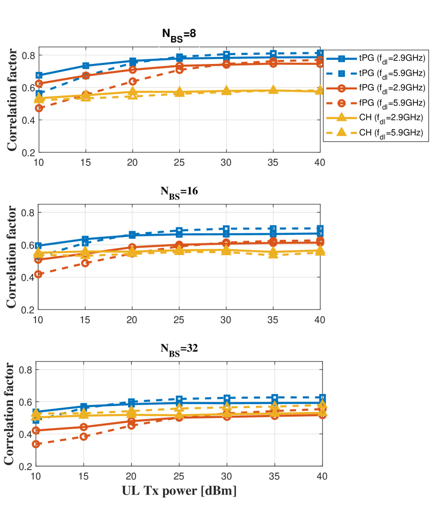
Fig. 8 shows the effect of UL parameter estimation errors on the DL extrapolation. As shown in Fig. 8, the fPG-learning has more difficulty in the DL extrapolation than the tPG-learning at low UL transmit power. Since the fPG-learning extracts the path gains and AoDs from the extracted channel coefficients, it is more vulnerable to the UL parameter estimation errors than the tPG-learning. This result proves that the precise DL channel reconstruction highly depends on accurate UL channel estimates. The CH-learning, on the contrary, is not affected much from the UL transmit power since it just exploits the UL channel estimates without further processing, which makes more robust to the estimation error.

The carrier frequency and guard band can also affect the NN-based DL extrapolation. We evaluate with different carrier frequency in Fig. 9 and different guard bands in Fig. 10. In (II-B), the path gain $\alpha(f_{c})$ is the only channel parameter related to the carrier frequency. When the carrier frequency is high, Fig. 9 shows that the proposed PG learning requires to have more UL transmit power to work properly since the path gain $\alpha(f_{c})$ attenuates more rapidly at high carrier frequency. However, Fig. 10 shows that the guard band seems to barely affect the DL extrapolation. Even for the 0.5 GHz guard band, which might be larger than most of practical FDD systems, the NN-based DL extrapolation methods work well as for the 0.1 GHz guard band. As the number of antennas at the BS increases, the overall correlation factors decrease but the tendency according to the guard band is maintained.

The correlation factors of the tPG, fPG, and CH-learning are compared with the MS speed in Fig. 11. The overall results show that the accuracy decreases at high speed.¹¹1The simulation environments with different speeds are based on different cluster geometries while all three methods are tested with the same geometry for the same speed. Therefore, lower speeds do not always give higher correlation factors due to different cluster geometries. The result of each speed is averaged over ten different geometries. When the MS speed is high, it may not be able for the MS to collect sufficient number of samples for the given length of the path since the snapshots of each MS sample set are generated every 40 msec. This problem can be resolved by increasing the number of MS sample sets. In Fig. 11, we train each learning method with 40, 100, and 200 MS sample sets. With 40 MS sample sets, the CH-learning suffers from insufficient number of data for training. On the contrary, the PG-learning is robust to the lack of samples. In addition, the accuracy of PG-learning is quite stable even at high speed compared to the CH-learning, which proves that the PG-learning is easier to train.

Note that the channel of MS with high speed could be outdated easily during the processing delay $d$. Since we have already taken $d$ into account for the training, the processing delay does not affect the accuracy even at high speed.

To compare the DL spectral efficiencies of the DL training and the NN-based DL extrapolation techniques, the coherence block length in (12) is derived as

where $f_{\mathrm{coh}}$ is the coherence bandwidth, which is set to 180 kHz as in Table I, and $T_{\mathrm{coh}}$ is the coherence time defined as

In (31), $c$ is the speed of light, $f_{c}$ is the DL carrier frequency, and $v$ is the speed of MS. The DL training overhead is $N_{\mathrm{BS}}$, and the transmit power at the BS is set to 30 dBm. For the DL training, we assume that the estimated DL CSI at the MS is perfectly fed back to the BS.

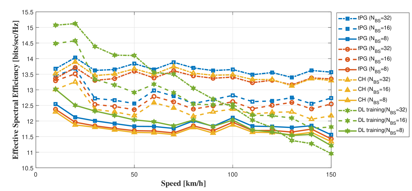
From Fig. 12, it is clear that the DL training suffers from large training overhead at high speed due to the short coherence block length. The performance degradation of DL training is especially severe when the number of BS antennas, $N_{\mathrm{BS}}$, is large, making it unsuitable to massive MIMO. This is quite clear from (9), i.e., with higher MS speed, the coherence block length decreases, and with more BS antennas, the training overhead increases. On the contrary, the NN-based DL extrapolation does not suffer from any DL training overhead. Moreover, as discussed in the previous subsection, the NN-based DL extrapolation does not suffer much for high MS speed by taking the processing delay into consideration for the training. The performance gap between the DL training and DL extrapolation would become even more prominent once we consider the limited feedback. Note that the proposed tPG-learning is always superior to the CH-learning while the fPG-learning and the CH-learning are comparable with each other.

References

- [1] E. G. Larsson, O. Edfors, F. Tufvesson, and T. L. Marzetta, “Massive MIMO for Next Generation Wireless Systems,” IEEE Commun. Mag., vol. 52, no. 2, pp. 186-195, Feb. 2014.
- [2] D. J. Love, R. W. Heath, V. K. N. Lau, D. Gesbert, B. D. Rao, and M. Andrews, “An Overview of Limited Feedback in Wireless Communication Systems,” IEEE J. Sel. Areas Commun., vol. 26, no. 8, pp. 1341-1365, Oct. 2008.
- [3] B. Hassibi, and B. M. Hochwald, “How Much Training is Needed in Multiple-Antenna Wireless Links?,” IEEE Trans. Inf. Theory, vol. 49, no. 4, pp. 951-963, Apr. 2003.
- [4] N. Jindal, “MIMO Broadcast Channels With Finite-Rate Feedback,” IEEE Trans. Inf. Theory, vol. 52, no. 11, pp. 5045-5060, Nov. 2006.
- [5] T. L. Marzetta, “Massive MIMO: An Introduction,” Bell Labs Technical Journal, vol. 20, pp. 11-22, 2015.
- [6] J. Choi, Z. Chance, D. J. Love, and U. Madhow, “Noncoherent Trellis Coded Quantization: A Practical Limited Feedback Techniques for Massive MIMO Systems,” IEEE Trans. Commun., vol. 61, no. 12, pp. 5016-5029, Dec. 2013.
- [7] A. Adhikary, J. Nam, J. Ahn, and G. Caire, “Joint Spatial Division and Multiplexing-The Large-Scale Array Regime,” IEEE Trans. Inf. Theory, vol. 59, no. 10, pp. 6441-6463, Oct. 2013.
- [8] J. Choi, D. J. Love, and P. Bidigare, “Downlink Training Technique for FDD Massive MIMO Systems: Open-Loop and Closed-Loop Training With Memory,” IEEE J. Sel. Topics Signal Process., vol. 8, no. 5, pp. 802-814, Oct. 2014.
- [9] S. Noh, M. D. Zoltowski, Y. Sung, D. J. Love, “Pilot Beam Pattern Design for Channel Estimation in Massive MIMO Systems,” IEEE J. Sel. Topics Signal Process., vol. 8, no. 5, pp. 787-801, Oct. 2014.
- [10] Z. Gao, L. Dai, Z. Wang, and S. Chen, “Spatially Common Sparsity Based Adaptive Channel Estimation and Feedback for FDD Massive MIMO,” IEEE Trans. Signal Process., vol. 63, no. 23, pp. 6169-6183, Dec. 2015.
- [11] C. Sun, X. Gao, S. Jin, M. Matthaiou, Z. Ding, and C. Xiao, “Beam Division Multiple Access Transmission for Massive MIMO,” IEEE Trans. Commun., vol. 63, no. 6, pp. 2170-2184, June 2015.
- [12] Z. Gao, L. Dai, W. Dai, B. Shim, and Z. Wang, “Structured Compressive Sensing-Based Spatio-Temporal Joint Channel Estimation for FDD Massive MIMO,” IEEE Trans. Commun., vol. 64, no. 2, pp. 601-617, Feb. 2016.
- [13] F. Rottenberg, R. Wang, J. Zhang, and A. F. Molisch, “Channel Extrapolation in FDD Massive MIMO: Theoretical Analysis and Numerical Validation,” 2019 arXiv:1902.06844, [Online]. Available: http://arxiv.org/abs/1902.06844.
- [14] M. Arnold, S. Dörner, S. Cammerer, S. Yan, J. Hoydis, and S. ten Brink, “Enabling FDD Massive MIMO through Deep Learning-based Channel Prediction,” 2019 arXiv:1901.03664, [Online]. Available: http://arxiv.org/abs/1901.03664.
- [15] M. Alrabeiah and A. Alkhateeb, “Deep Learning for TDD and FDD Masive MIMO: Mapping Channels in Space and Frequency,” 2019 arXiv:1905.03761, [Online]. Available: http://arxiv.org/abs/1905.03761.
- [16] Y. Yang, F. Gao, G. Y. Li, and M. Jian, “Deep Learning-Based Downlink Channel Prediction for FDD Massive MIMO System,” IEEE Commun. Lett., vol. 23, no. 11, pp. 1994-1998, Nov. 2019.
- [17] D. Vasisht, S. Kumar, H. Rahul, and D. Katabi, “Eliminating Channel Feedback in Next-Generation Cellular Networks,” Proceedings of the 2016 ACM SIGCOMM Conference, pp. 398-411, 2016.
- [18] X. Li and A. Alkhateeb, “Deep Learning for Direct Hybrid Precoding in Millimeter Wave Massive MIMO Systems,” 2019 arXiv:1905.13212, [Online]. Available: http://arxiv.org/abs/1905.13212.
- [19] C. Wen, W. Shih, and S. Jin, “Deep Learning for Massive MIMO CSI Feedback,” IEEE Wireless Commun. Lett., vol. 7, no. 5, pp. 748-751, Oct. 2018.
- [20] A. M. Elbir, “CNN-Based Precoder and Combiner Design in mmWave MIMO Systems,” IEEE Commun. Lett., vol. 23, no. 7, pp. 1240-1243, July 2019.
- [21] H. Huang, Y. Peng, J. Yang, W. Xia, and G. Gui, ”Fast Beamforming Design via Deep Learning,” IEEE Trans. Veh. Technol., vol. 69, no. 1, pp. 1065-1069, Oct. 2019.
- [22] Y. Wang, M. Liu, J. Yang, and G. Gui, ”Data-Driven Deep Learning for Automatic Modulation Recognition in Cognitive Radios,” IEEE Trans. Veh. Technol., vol. 68, no. 4, pp. 4074-4077, Feb. 2019.
- [23] S. Jaeckel, L. Raschkowski, K. Börner, and L. Thiele, “QuaDRiGa: A 3-D Multi-Cell Channel Model with Time Evolution for Enabling Virtual Field Trials,” IEEE Trans. Antennas Propag., vol. 62, no. 6, pp. 3242-3256, June 2014.
- [24] Wireless InSite. Remcom Corp., 2019. [Online]. Available: https://www.remcom.com/wireless-insite-em-propagation-software. Accessed on: Dec. 2, 2019.
- [25] P. Dong, H. Zhang, G. Y. Li, I. S. Gaspar, and N. NaderiAlizadeh, “Deep CNN-Based Channel Estimation for mmWave Massive MIMO Systems,” IEEE J. Sel. Topics Signal Process., vol. 13, no. 5, pp. 989-1000, Sep. 2019.
- [26] J. Vieira, E. Leitinger, M. Sarajlic, X. Li, and F. Tufvesson, “Deep Convolutional Neural Networks for Massive MIMO Fingerprint-based Positioning,” Proceedings of IEEE International Symposium on Personal, Indoor, and Mobile Radio Communications, pp. 1-6, Oct. 2017.
- [27] J. Choi, G. Lee, and B. L. Evans, “Two-Stage Analog Combining in Hybrid Beamforming Systems With Low-Resolution ADCs,” IEEE Trans. Signal Process., vol. 67, no. 9, pp. 2410-2425, May 2019.
- [28] S. Navabi, C. Wang, O. Y. Bursalioglu, and H. Papadopoulos, “Predicting Wireless Channel Features Using Neural Networks,” Proceedings of IEEE International Conference on Communications, pp. 1-6, May 2018.
- [29] A. Géron, “Convolutional Neural Networks,” in Hands-On Machine Learning with Scikit-Learn, Keras, and TensorFlow: Concepts, Tools, and Techniques to Build Intelligent Systems, 1st ed., Sebastopol, CA, USA: O’Reilly Media, 2017, pp. 355–380.
- [30] S. B. Driss, M. Soua, R. Kachouri, and M. Akil, “A Comparison Study Between MLP and Convolutional Neural Network Models for Character Recognition,” Proceedings of Real-Time Image and Video Processing 2017, vol. 10223, pp. 1023306. International Society for Optics and Photonics, 2017.
- [31] Y. Chi and M. F. Da Costa, “Harnessing Sparsity over the Continuum: Atomic Norm Minimization for Super Resolution,” 2019 arXiv:1904.04283, [Online]. Available: http://arxiv.org/abs/1904.04283.
- [32] J. Ma, S. Zhang, H. Li, F. Gao, and S. Jin, “Sparse Bayesian Learning for the Time-Varying Massive MIMO Channels: Acquisition and Tracking,” IEEE Trans. Commun., vol. 67, no. 3, pp. 1925-1938, Mar. 2019.
- [33] M. Li, S. Zhang, N. Zhao, W. Zhang, and X. Wang, “Time-Varying Massive MIMO Channel Estimation: Capturing, Reconstruction, and Restoration,” IEEE Trans. Commun., vol. 67, no. 11, pp. 7558-7572, Nov. 2019. F
- [34] J. Zhao, H. Xie, F. Gao, W. Jia, S. Jin, and H. Lin, “Time Varying Channel Tracking With Spatial and Temporal BEM for Massive MIMO Systems,” IEEE Trans. Wireless Commun., vol. 17, no. 8, pp. 5653-5665, Aug. 2018.
- [35] Y. Han, Q. Liu, C.-K. Wen, M. Matthaiou, and X. Ma, “Tracking FDD Massive MIMO Downlink Channels by Exploiting Delay and Angular Reciprocity,” IEEE J. Sel. Topics Signal Process., vol. 13, no. 5, pp. 1062-1076, Sep. 2019.
- [36] G. Gui, H. Huang, Y. Song, and H. Sari, ”Deep Learning for an Effective Nonorthogonal Multiple Access Scheme,” IEEE Trans. Veh. Technol., vol. 67, no. 9, pp. 8440-8450, June 2018.