Doubly Robust Interval Estimation for Optimal Policy Evaluation in Online Learning
Abstract
Evaluating the performance of an ongoing policy plays a vital role in many areas such as medicine and economics, to provide crucial instructions on the early-stop of the online experiment and timely feedback from the environment. Policy evaluation in online learning thus attracts increasing attention by inferring the mean outcome of the optimal policy (i.e., the value) in real-time. Yet, such a problem is particularly challenging due to the dependent data generated in the online environment, the unknown optimal policy, and the complex exploration and exploitation trade-off in the adaptive experiment. In this paper, we aim to overcome these difficulties in policy evaluation for online learning. We explicitly derive the probability of exploration that quantifies the probability of exploring non-optimal actions under commonly used bandit algorithms. We use this probability to conduct valid inference on the online conditional mean estimator under each action and develop the doubly robust interval estimation (DREAM) method to infer the value under the estimated optimal policy in online learning. The proposed value estimator provides double protection for consistency and is asymptotically normal with a Wald-type confidence interval provided. Extensive simulation studies and real data applications are conducted to demonstrate the empirical validity of the proposed DREAM method.
Keywords: Asymptotic Normality; Bandit Algorithms; Double Protection; Online Estimation; Probability of Exploration
1 Introduction
Sequential decision-making is one of the essential components of modern artificial intelligence that considers the dynamics of the real world. By maintaining the trade-off between exploration and exploitation based on historical information, bandit algorithms aim to maximize the cumulative outcome of interest and are thus popular in dynamic decision optimization with a wide variety of applications, such as precision medicine (Lu et al., 2021) and dynamic pricing (Turvey, 2017). There has been a vast literature on bandit optimization established over recent decades (see e.g., Sutton and Barto, 2018; Lattimore and Szepesvári, 2020, and the references therein). Most of these theoretical works focus on the regret analysis of bandit algorithms. When properly designed and implemented to address the exploration-and-exploitation trade-off, a powerful bandit policy could achieve a sub-linear regret, and thus eventually approximate the underlying optimal policy that maximizes the expected outcome. However, such a regret analysis only shows the convergence rate of the averaged cumulative regret (difference between the outcome under the optimal policy and that under the bandit policy) but provides limited information on the expected outcome under this bandit policy (referred to as the value in Dudík et al. (2011)).
The evaluation of the performance of bandit policies plays a vital role in many areas, including medicine and economics (see e.g., Chakraborty and Moodie, 2013; Athey, 2019). By evaluation, we aim to unbiasedly estimate the value of the optimal policy that the bandit policy is approaching and infer the corresponding estimate. Although there is an increasing trend in policy evaluation (see e.g., Li et al., 2011; Dudík et al., 2011; Swaminathan et al., 2017; Wang et al., 2017; Kallus and Zhou, 2018; Su et al., 2019), we note that all of these works focus on learning the value of a target policy offline using historical log data. See the architecture of offline policy evaluation illustrated in the left panel of Figure 1. Instead of a post-experiment investigation, it has attracted more attention recently to evaluate the ongoing policy in real-time. In precision medicine, the physician aims to make the best treatment decision for each patient sequentially according to their baseline covariates. Estimating the mean outcome of the current treatment decision rule is crucial to answering several fundamental questions in health care, such as whether the current strategy significantly optimizes patient outcomes over some baseline strategies. When the value under the ongoing rule is much lower than the desired average curative effect, the online trial must be terminated until more effective treatment options are available for the next round. Thus, policy evaluation in online learning is a new idea to provide the early stop of the online experiment and timely feedback from the environment, as demonstrated in the right panel of Figure 1.


1.1 Related Works and Challenges
Despite the importance of policy evaluation in online learning, the current bandit literature suffers from three main challenges. First, the data, such as the actions and rewards sequentially collected from the online environment, are not independent and identically distributed (i.i.d.) since they depend on the previous history and the running policy (see the right panel of Figure 1). In contrast, the existing methods for the offline policy evaluation (see e.g., Li et al., 2011; Dudík et al., 2011) primarily assumed that the data are generated by the same behavior policy and i.i.d. across different individuals and time points. Such assumptions allow them to evaluate a new policy using offline data by modeling the behavior policy or the conditional mean outcome. In addition, we note that the target policy to be evaluated in offline policy evaluation is fixed and generally known, whereas for policy evaluation in online learning, the optimal policy of interest needs to be estimated and updated in real time.
The second challenge lies in estimating the mean outcome under the optimal policy online. Although numerous methods have recently been proposed to evaluate the online sample mean for a fixed action (see e.g., Nie et al., 2018; Neel and Roth, 2018; Deshpande et al., 2018; Shin et al., 2019a, b; Waisman et al., 2019; Hadad et al., 2019; Zhang et al., 2020), none of these methods is directly applicable to our problem, as the sample mean only provides the impact of one particular arm, not the value of the optimal policy in bandits that considers the dynamics of the online environment. For instance, in the contextual bandits, we aim to select an action for each subject based on its context/feature to optimize the overall outcome of interest. However, there may not exist a unified best action for all subjects due to heterogeneity, and thus evaluating the value of one single optimal action cannot fully address the policy evaluation in such a setting. However, although commonly used in the regret analysis, the average of collected outcomes is not a good estimator of the value under the optimal policy in the sense that it does not possess statistical efficiency (see details in Section 3).
Third, given data generated by a bandit algorithm that maintains the exploration-and-exploitation trade-off sequentially, inferring the value of the optimal policy online should consider such a trade-off and quantify the probability of exploration and exploitation. The probability of exploring non-optimal actions is essential in two ways. First, it determines the convergence rate of the online conditional mean estimator under each action. Second, it indicates the data points used to match the value under the optimal policy. To our knowledge, the regret analysis in the current bandit literature is based on the binding of variance information (see e.g., Auer, 2002; Srinivas et al., 2009; Chu et al., 2011; Abbasi-Yadkori et al., 2011; Bubeck and Cesa-Bianchi, 2012; Zhou, 2015), yet little effort has been made in formally quantifying the probability of exploration over time.
There are very few studies directly related to our topic. Chambaz et al. (2017) established the asymptotic normality for the conditional mean outcome under an optimal policy for sequential decision making. Later, Chen et al. (2020) proposed an inverse probability weighted value estimator to infer the value of optimal policy using the -Greedy (EG) method. These two works did not discuss how to account for the exploration-and-exploitation trade-off under commonly used bandit algorithms, such as Upper Confidence Bound (UCB) and Thompson Sampling (TS), as considered in this paper. Recently, to evaluate the value of a known policy based on the adaptive data, Bibaut et al. (2021) and Zhan et al. (2021) proposed to utilize the stabilized doubly robust estimator and the adaptive weighting doubly robust estimator, respectively. However, both methods focused on obtaining a valid inference of the value estimator under a fixed policy by conveniently assuming a desired exploration rate to ensure sufficient sampling of different arms. Such an assumption can be violated in many commonly used bandits (see details shown in Theorem 4.1). Although there are other works that focus on statistical inference for adaptively collected data (Dimakopoulou et al., 2021; Zhang et al., 2021; Khamaru et al., 2021; Ramprasad et al., 2022) in bandit or reinforcement learning setting, our work handles policy evaluation from a completely unique angle to infer the value of optimal policy by investigating the exploration rate in online learning.
1.2 Our Contributions
In this paper, we aim to overcome the aforementioned difficulties of policy evaluation in online decision-making. Our contributions are expressed in the following folds.
The first contribution of this work is to explicitly characterize the trade-off between exploration and exploitation in the online policy optimization, we derive the probability of exploration in bandit algorithms. Such a probability is new to the literature by quantifying the chance of taking the nongreedy policy (i.e., a nonoptimal action) given the current information over time, in contrast to the probability of exploitation for taking greedy actions. Specifically, we consider three commonly used bandit algorithms for exposition, including the UCB, TS, and EG methods. We note that the probability of exploration is prespecified by users in EG while remaining implicit in UCB and TS. We use this probability to conduct valid inferences on the online conditional mean estimator under each action. The second contribution of this work is to propose the doubly robust interval estimation (DREAM) to infer the mean outcome of the optimal online policy. The DREAM provides double protection on the consistency of the proposed value estimator to the true value, given the product of the nuisance error rates of the probability of exploitation and the conditional mean outcome as for as the termination time. Under standard assumptions for inferring the online sample mean, we show that the value estimator under DREAM is asymptotically normal with a Wald-type confidence interval provided. To the best of our knowledge, this is the first work to establish the inference for the value under the optimal policy by taking the exploration-and-exploitation trade-off into thorough account and thus fills a crucial gap in the policy evaluation of online learning.
The remainder of this paper is organized as follows. We introduce notation and formulate our problem, followed by preliminaries of standard contextual bandit algorithms and the formal definition of probability of exploration. In Section 3, we introduce the DREAM method and its implementation details. Then in Section 4, we derive theoretical results of DREAM under contextual bandits by establishing the convergence rate of the probability of exploration and deriving the asymptotic normality of the online mean estimator. Extensive simulation studies are conducted to demonstrate the empirical performance of the proposed method in Section 5, followed by a real application using OpenML datasets in Section 6. We conclude our paper in Section 7 by discussing the performance of the proposed DREAM in terms of the regret bound and a direct extension of our method for policy evaluation of any known policy in online learning. All the additional results and technical proofs are given in the appendix.
2 Problem Formulation
In this section, we formulate the problem of policy evaluation in online learning. We first build the framework based on the contextual bandits in Section 2.1. We then introduce three commonly used bandit algorithms, including UCB, TS, and EG, to generate data online, in Section 2.2. Lastly, we define the probability of exploration in Section 2.3. In this paper, we use bold symbols for vectors and matrices.
2.1 Framework
In contextual bandits, at each time step , we observe a -dimensional context drawn from a distribution which includes 1 for the intercept, choose an action , and then observe a reward . Denote the history observations prior to time step as . Suppose that the reward given and follows , where is the conditional mean outcome function (also known as the Q-function in the literature (Murphy, 2003; Sutton and Barto, 2018)), and is bounded by . The noise term is independent -subgaussian at the time step independently of given for . Let the conditional variance be . The value (Dudík et al., 2011) of a given policy is defined as
We define the optimal policy as , which finds the optimal action based on the conditional mean outcome function given a context . Thus, the optimal value can be defined as . In the rest of this paper, to simplify the exposition, we focus on two actions, that is, . Then the optimal policy is given by
Our goal is to infer the value under the optimal policy using the online data sequentially generated by a bandit algorithm. Since the optimal policy is unknown, we estimate the optimal policy from the online data as . As commonly assumed in the current online inference literature (see e.g., Deshpande et al., 2018; Zhang et al., 2020; Chen et al., 2020) and the bandit literature (see e.g., Chu et al., 2011; Abbasi-Yadkori et al., 2011; Bubeck and Cesa-Bianchi, 2012; Zhou, 2015), we consider the conditional mean outcome function taking a linear form, i.e., where is a smooth function and can be estimated via a ridge regression based on as
| (1) |
where is a identity matrix, is a design matrix at time with as the number of pulls for action , is the vector of the outcomes received under action at time , and is a positive and bounded constant as the regularization term. There are two main reasons to choose the ridge estimator instead of the ordinary least squares estimator that is considered in Deshpande et al. (2018); Zhang et al. (2020); Chen et al. (2020). First, the ridge estimator is well defined when is singular and its bias is negligible when the time step is large. Second, the parameter estimations in the ridge method are in accordance with the linear UCB (Li et al., 2010) and the linear TS (Agrawal and Goyal, 2013) methods (detailed in the next section) with . Based on the ridge estimator in (1), the online conditional mean estimator for is defined as . With two actions, the estimated optimal policy at time step is defined by
| (2) |
We note that the linear form of can be relaxed to the non-linear case as , where is a continuous function (see examples in our simulation studies in Section 5). Then the corresponding online conditional mean estimator for is defined as based on .
2.2 Bandit Algorithms
We briefly introduce three commonly used bandit algorithms in the framework of contextual bandits, to generate the online data sequentially.
Upper Confidence Bound (UCB) (Li et al., 2010): Let the estimated standard deviation based on be The action at time is selected by
where is a non-increasing positive parameter that controls the level of exploration. With two actions, we have the action at time step as
Thompson Sampling (TS) (Agrawal and Goyal, 2013): Suppose a normal likelihood function for the reward given and such that with a known parameter . If the prior for at time is
where is the -dimensional multivariate normal distribution, we have the posterior distribution of as
for .
At each time step , we draw a sample from the posterior distribution as for ,
and select the next action within two arms by
-Greedy (EG) (Sutton and Barto, 2018): Recall the estimated conditional mean outcome for action as given a context .
Under EG method, the action at time is selected by
where and the parameter controls the level of exploration as pre-specified by users.
2.3 Probability of Exploration
We next quantify the probability of exploring non-optimal actions at each time step. To be specific, define the status of exploration as , indicating whether the action taken by the bandit algorithm is different from the estimated optimal action that exploits the historical information, given the context information. Here, can be viewed as the greedy policy at time step . Thus the probability of exploration is defined by
| (3) |
where the expectation in the last term is taken respect to and history . According to (3), is determined by the given context information and the current time point. We clarify the connections and distinctions of the defined probability of exploration concerning the bandit literature here. First, the exploration rate used in the current bandit works mainly refers to the probability of exploring non-optimal actions given an optimal policy and contextual information at time step , i.e., . This is different from our proposed probability of exploration . The main difference lies in the estimated optimal policy from the collected data at the current time step , i.e., , in . If properly designed and implemented, the estimated optimal policy under a bandit algorithm will eventually converge to the true optimal policy when is large, which yields . In practice, we can estimate sequentially by using as inputs and as outputs via parametric or non-parametric tools. We denote the corresponding estimator as for time step . Such implementation conditions are explicitly described in Section 3.
3 Doubly Robust Interval Estimation
We present the proposed DREAM method in this section. We first detail why the average of outcomes received in bandits fails to process statistical efficiency. In view of the results established in regret analysis for the contextual bandits (see e.g., Abbasi-Yadkori et al., 2011; Chu et al., 2011; Zhou, 2015), we have the cumulative regret as , where is the asymptotic order up to some logarithm factor. Therefore, it is immediate that the average of rewards follows , since the dimension is finite. These results indicate that a simple average of the total outcome under the bandit algorithm is not a good estimator for the optimal value, since it does not own the asymptotic normality for a valid confidence interval construction. Instead of the simple aggregation, intuitively, we should select the outcome when the action taken under a bandit policy accords with the optimal policy, i.e., , defined as the status of exploitation. In contrast to the probability of exploration, we define the probability of exploitation as
Following the doubly robust value estimator in Dudík et al. (2011), we propose the doubly robust mean outcome estimator as the value estimator under the optimal policy as
| (4) |
where is the current/termination time, and is the estimated matching probability between the chosen action and estimated optimal action given , which captures the probability of exploitation. Our value estimator provides double protection on the consistency to the true value, given the product of the nuisance error rates of the probability of exploitation and the conditional mean outcome as , as discussed in Theorem 3. We further propose a variance estimator for as
|
|
(5) |
where is an estimator for , for . The proposed variance estimator is consistent to the true variance of the value shown in Theorem 3. We officially name our method as doubly robust interval estimation (DREAM), with the detailed pseudocode provided in Algorithm 1. To ensure sufficient exploration and a valid inference, we force to pull non-optimal actions given greedy samples with a pre-specified clipping rate in step (4) of Algorithm 1 of an order larger than as required by Theorem 3. In step (4), if the unchosen action does not satisfy the clipping condition detailed in Assumption 4.2, then we will force to pull this non-greedy action for additional exploration, as required for a valid online inference. The estimated probability of exploration is used in step (6) in Algorithm 1 to learn the value and variance. A potential limitation of DREAM rises when the agent resists taking extra non-greedy actions in online learning. Yet, we discuss in Section 7.1 that the regret from such an extra exploration is negligible compared to the regret from exploitation, thus we can still maintain the sub-linear regret under DREAM. The theoretical validity of the proposed DREAM is detailed in Section 4, with its empirical out-performance over baseline methods demonstrated in Section 5. Finally, we remark that our method is not overly sensitive to the choice of with additional sensitivity analyses provided in Appendix A.
4 Theoretical Results
We formally present our theoretical results. In Section 4.1, we first derive the bound of the probability of exploration under the three commonly used bandit algorithms introduced in Section 2.2. This allows us to further establish the asymptotic normality of the online conditional mean estimator under a specific action in Section 4.2. Next, we establish the theoretical properties of DREAM with a Wald-type confidence interval given in Section 4.3. All the proofs are provided in Appendix B. The following assumptions are required to establish our theories.
Assumption 4.1
(Boundness) There exists a positive constant such that for all , and has minimum eigenvalue for some .
Assumption 4.2
(Clipping) For any action and time step , there exists an sequence positive and non-increasing , such that
Assumption 4.3
(Margin Condition) Assume there exist some constants and such that , where the big-O term is uniform in .
Assumption 4.1 is a technical condition on bounded contexts such that the mean of the martingale differences will converge to zero (see e.g., Zhang et al., 2020; Chen et al., 2020). Assumption 4.2 is a technical requirement for the uniqueness and convergence of the least squares estimators, which requires the bandit algorithm to explore all actions sufficiently such that the asymptotic properties for the online conditional mean estimator under different actions hold (see e.g., Deshpande et al., 2018; Hadad et al., 2019; Zhang et al., 2020). The parameter defined in Assumption 4.2 characterizes the boundary of the probability of taking one action and we name it as the clipping rate. We ensure Assumption 4.2 is satisfied using step (4) in Algorithm 1. We establish the relationship between and and discuss the requirement for to consistently estimate in this section. Assumption 4.3 is well known as the margin condition, which is commonly assumed in the literature to derive a sharp convergence rate for the value under the estimated optimal policy (see e.g., Luedtke and Van Der Laan, 2016; Chambaz et al., 2017; Chen et al., 2020).
4.1 Bounding the Probability of Exploration
The probability of exploration not only shows the signal of success in finding the global optimization in online learning, but also connects to optimal policy evaluation by quantifying the rate of executing the greedy actions. Instead of directly specifying this probability (see e.g., Zhang et al., 2020; Chen et al., 2020; Bibaut et al., 2021; Zhan et al., 2021), we explicitly bound this rate based on the updating parameters in bandit algorithms, by which we conduct a valid follow-up inference. Since the probability of exploration involves the estimation of the mean outcome function, we need to first derive a tail bound for the online ridge estimator and the estimated difference between the mean outcomes.
Lemma 4.1
The results in Lemma 4.1 establish the tail bound of the online ridge estimator , which can be simplified as , for some constants , by noticing the constant and , the dimension , the subgaussian parameter , and the bound are positive and bounded, under bounded true coefficients . Recall the clipping constraint that is non-increasing sequence. This tail bound is asymptotically equivalent to . The established results in Lemma 4.1 work for general bandit algorithms including UCB, TS, and EG. These tail bounds are aligned with the bound derived in Chen et al. (2020) for the EG method only. By Lemma 4.1, it is immediate to obtain the consistency of the online ridge estimator , if as . We can further obtain the tail bound for the estimated difference between the conditional mean outcomes under two actions by Lemma 4.1 as detailed in the following corollary.
Corollary 1
(Tail bound for the online mean estimator) Suppose conditions in Lemma 4.1 hold. Denote , then for any , we have the probability of the online conditional mean estimator bounded within its true as
with
being a constant of time .
The above corollary quantifies the uncertainty of the online estimation of the conditional mean outcomes, and thus provides a crucial middle result to further access the probability of exploration by noting in (2). More specifically, we derive the probability of exploration at each time step under the three discussed bandit algorithms for exposition in the following theorem.
Theorem 1
(Probability of exploration)
In the online contextual bandit algorithms using UCB, TS, or EG, given a context at time step , assuming Assumptions 4.1, 4.2, and 4.3 hold with , then for any with specified in Corollary 1,
(i) under UCB, there exists some constant such that
(ii) under TS, we have
(iii) under EG, we have .
The theoretical order of is new to the literature, which quantifies the probability of exploring the non-optimal actions under a bandit policy over time. We note that the probability of exploration under EG is pre-specified by users, which directly implies its exploring rate as (for the two-arm setting) as shown in results (iii). The results (i) and (ii) in Theorem 1 show that the probabilities of exploration under UCB and TS are non-increasing under certain conditions. For instance, if for TS, as , the upper bound for decays to zero with an asymptotically equivalent convergence rate as up to some constant. Similarly, for UCB, with an arbitrarily small at an order of , as , the upper bound for decays to zero as long as . Theorem 1 also indicates that without the clipping required in Assumption 4.2 and implemented in step (4) of Algorithm 1, the exploration for non-optimal arms might be insufficient, leading to a possibly invalid and biased inference for the online conditional mean.
4.2 Asymptotic Normality of Online Ridge Estimator
We use the established bounds for the probability of exploration in Theorem 1 to further obtain the asymptotic normality for the online conditional mean estimator under each action. Specifically, denote given a context . Assume the conditions in Theorem 1 hold and as , we have the upper bound of the probability of exploration decays to zero in Theorem 1 for UCB and TS. Since is nonnegative by its definition, it follows from Sandwich Theorem immediately that exist for UCB and TS, and for EG. By using this limit, we can further characterize the following theorem for asymptotics and inference.
Theorem 2
(Asymptotics and inference) Supposing the conditions in Theorem 1 hold with as , we have and for and , with the variance given by
The results in Theorem 2 establish the asymptotic normality of the online ridge estimator and the online conditional mean estimator over time, with an explicit asymptotic variance derived. Here, may differ under different bandit algorithms while the asymptotic normality holds as long as the adopted bandit algorithm explores the non-optimal actions sufficiently with a non-increasing rate, following the conclusion in Theorem 1, i.e., a clipping rate of an order larger than as described in Algorithm 1. The proof of Theorem 2 generalizes Theorem 3.1 in Chen et al. (2020) by additionally considering the online ridge estimator and general bandit algorithms.
4.3 Asymptotic Normality and Robustness for DREAM
In this section, we further derive the asymptotic normality of . The following additional assumption is required to establish the double robustness of DREAM.
Assumption 4.4
(Rate Double Robustness) Define as the norm. Let , and . Assume the product of two rates satisfies .
Assumption 4.4 requires the estimated conditional mean function and the estimated probability of exploration to converge at certain rates in online learning. This assumption is frequently studied in the causal inference literature (see e.g., Farrell, 2015; Luedtke and Van Der Laan, 2016; Smucler et al., 2019; Hou et al., 2021; Kennedy, 2022) to derive the asymptotic distribution of the estimated average treatment effect with either parametric estimators or non-parametric estimators (see e.g., Wager and Athey, 2018; Farrell et al., 2021). We remark that under the conditions required in Theorem 2, we have for all , thus Assumption 4.4 holds as along as . We then have the asymptotic normality of as stated in the following theorem.
Theorem 3
The above theorem shows that the value estimator under DREAM is doubly robust to the true value, given the product of the nuisance error rates of the probability of exploitation and the conditional mean outcome as . We use the Martingale Central Limit Theorem to overcome the non-i.i.d. sample problem for asymptotic normality. The asymptotic variance of the proposed estimator is caused by two sources. One is the variance due to the context information, and the other is a weighted average of the variance under the optimal arm and the variance under the non-optimal arms. The weight is determined by the probability of exploration when under the adopted bandit algorithm. To the best of our knowledge, this is the first work that studies the asymptotic distribution of the mean outcome of the estimated optimal policy under general online bandit algorithms, which takes the exploration-and-exploitation trade-off into a thorough account. Our method thus fills a crucial gap in policy evaluation of online learning. By Theorem 3, a two-sided confidence interval (CI) for is , where denotes the upper th quantile of a standard normal distribution.
5 Simulation Studies
We investigate the finite sample performance and demonstrate the coverage probabilities of the policy value of DREAM in this section. The computing infrastructure used is a virtual machine in the AWS Platform with 72 processor cores and 144GB memory.
Consider the 2-dimensional context , with . Suppose the outcome of interest given and is generated from , where the conditional mean function takes a non-linear form as , with equal variances as and . Then the optimal policy is given by , and the optimal value is 3.27 calculated by integration.
We employ the three bandit algorithms described in Section 2.2 to generate the online data with (Li et al., 2010), where for UCB, with for TS, and for EG. Set the total decision time as with a burning period .

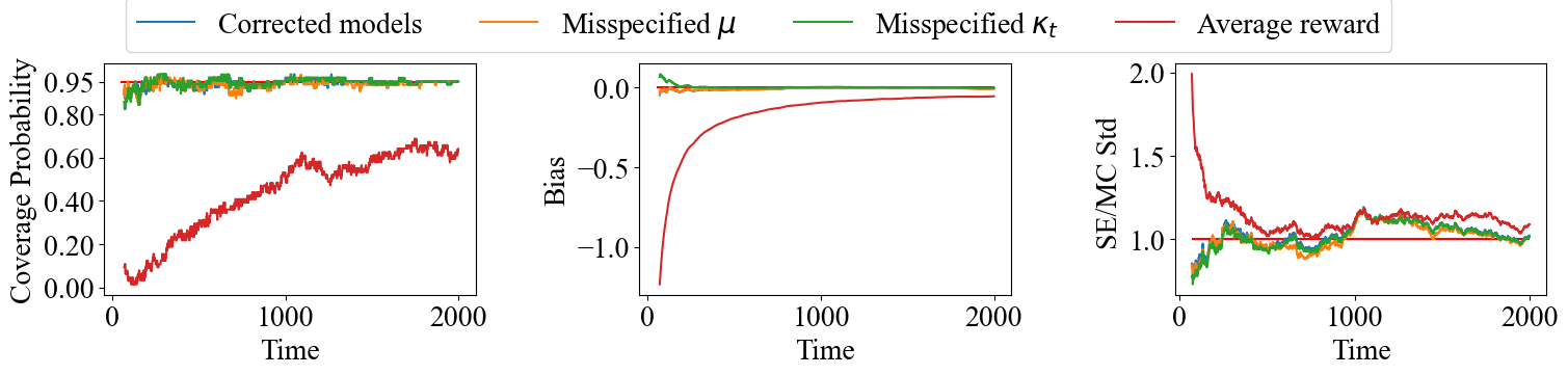
We evaluate the doubly robustness property of the proposed value estimator under DREAM in comparison to the simple average of the total reward for contextual bandits. To be specific, we consider the following four methods: 1. the conditional mean function is correctly specified, and the probability of exploration is estimated by a nonparametric regression in DREAM; 2. the probability of exploration is estimated by a nonparametric regression while the model of is misspecified with linear regression; 3. the conditional mean function is correctly specified while the model of is misspecified by a constant 0.5; 4. using the averaged reward as the value estimator. The clipping rate of DREAM is set to be 0.01, and our method is not overly sensitive to the choice of as shown in additional sensitivity analyses provided in Appendix A. The above four value estimators are evaluated by the coverage probabilities of the 95% two-sided Wald-type CI on covering the optimal value, the bias, and the ratio between the standard error and the Monte Carlo standard deviation, as shown in Figure 2 for UCB, Figure 3 for TS, and Figure 4 for EG, aggregated over 1000 runs.

Based on Figures 2, 3, and 4, the performance of the proposed DREAM method is reasonably much better than the simple average estimator of the total outcome. Specifically, under different bandit algorithms, when the time increases, the coverage probabilities of the proposed DREAM estimator are close to the nominal level of 95%, with the biases approaching 0 and the ratios between the standard error and the Monte Carlo standard deviation approaching 1. In addition, our DREAM method achieves reasonably good performance when either regression model for the conditional mean function or the probability of exploration is misspecified. These findings not only validate the theoretical results in Theorem 3 but also demonstrate the doubly robustness of DREAM in handling policy evaluation in online learning. In contrast, the simple average of reward can hardly maintain coverage probabilities over 80% with much larger biases in all cases.

6 Real Data Application
In this section, we evaluate the performance of the proposed DREAM method in real datasets from the OpenML database, which is a curated, comprehensive benchmark suite for machine-learning tasks. Following the contextual bandit setting considered in this paper, we select two datasets in the public OpenML Curated Classification benchmarking suite 2018 (OpenML-CC18; BSD 3-Clause license) (Bischl et al., 2017), i.e., the SEA50 and SEA50000, to formulate the real application. Each dataset is a collection of pairs of 3-dimensional features and their corresponding labels , with a total number of observations as 1,000,000. To simulate an online environment for data generation, we turn two-class classification tasks into two-armed contextual bandit problems (see e.g., Dudík et al., 2011; Wang et al., 2017; Su et al., 2019), such that we can reproduce the online data to evaluate the performance of the proposed method. Specifically, at each time step , we draw the pair uniformly at random without replacement from the dataset with 1,000,000. Given the revealed context , the bandit algorithm selects an action . The reward is generated by a normal distribution . Here, the mean of reward is 1 if the selected action matches the underlying true label, and 0 otherwise. Therefore, the optimal value is 1 while the optimal policy is unknown due to the complex relationship between the collected features and the label. Our goal is to infer the value under the optimal policy in the online settings produced by datasets SEA50 and SEA50000.

Using the similar procedure as described in Section 5, we apply DREAM in comparison to the simple average estimator, by employing three bandit algorithms with the following specifications: (i) for UCB, let ; (ii) for TS, let priors and parameter ; and (iii) for EG, let . Set the total time for the online learning as with a burning period as . The results are evaluated by the coverage probabilities of the 95% two-sided Wald-type CI in Figure 5 for two real datasets, respectively, averaged over 500 replications. It can be observed from Figure 5 that our proposed DREAM method performs much better than the simple average estimator, in all cases. To be specific, the coverage probabilities of the value estimator under DREAM are close to the nominal level of 95%, while the CI constructed by the averaged reward can hardly cover the true value with its coverage probabilities decaying to 0, under different bandit algorithms and two simulated online environments. These findings are consistent with what we have observed in simulations and consolidate the practical usefulness of the proposed DREAM.
7 Discussion
In this paper, we propose doubly robust interval estimation (DREAM) to infer the mean outcome of the optimal policy using the online data generated from a bandit algorithm. We explicitly characterize the probability of exploring the non-optimal actions under different bandit algorithms and show the consistency and asymptotic normality of the proposed value estimator. In this section, we discuss the performance of DREAM in terms of the regret bound and extend it to the evaluation of a known policy in online learning.
7.1 Regret Bound under DREAM
In this section, we discuss the regret bound of the proposed DREAM method. Specifically, we study the regret defined as the difference between the expected cumulative rewards under the oracle optimal policy and the bandit policy, which is
| (6) |
By noticing that if and 0 otherwise, we have
We note that the indicator function is equivalent to and is bounded by . Thus, we can divide the regret defined in Equation (6) into two parts as where
is the regret from the exploration and is the regret from the exploitation. It is well known that the regret from the exploitation is sublinear (Chu et al., 2011; Agrawal and Goyal, 2013) and the regret for EG has been well studied by Chen et al. (2020). Therefore, we focus on the analysis of the regret from the exploration for UCB and TS here.
Since is bounded and the upper bound of has an asymptotically equivalent convergence rate as up to some constant by Theorem 1, there exists some constant such that the regret from the exploration is bounded by
If we choose for some , the regret is bounded by , where the equation is calculated using Lemma 6 in Luedtke and Van Der Laan (2016). Thus, we still have sublinear regret under DREAM.
7.2 Evaluation of Known Policies in Online Learning
We could extend our method to evaluate a new known policy that is different from the bandit policy, in the online environment. Typically, we focus on the statistical inference of policy evaluation in online learning under the contextual bandit framework. Recall the setting and notations in Section 2, given a target policy , we propose its doubly robust value estimator as
where is the current time step or the termination time and is the estimator for the propensity score of the chosen action denoted as . The following theorem summarizes the asymptotic properties of , built on Theorem 2.
Corollary 2
(Asymptotic normality for evaluating a known policy) Suppose the conditions in Theorem 2 hold. Furthermore, assuming the rate doubly robustness that we have , with
where .
Here, we impose the same conditions on the bandit algorithms as in Theorem 3 to guarantee sufficient exploration on different arms, and thus evaluating an arbitrary policy is valid. The usage of the new rate doubly robustness assumption and the margin condition (Assumption 4.3) follows a similar logic as in Theorem 3. The estimator of denoted as can be obtained similarly to (5). Thus, a two-sided CI for under online optimization is .
There are some other extensions that we may also consider in future work. First, in this paper, we focus on settings with binary actions. Thus, a more general method with multiple actions or even a continuous action space is desirable. Second, we consider the contextual bandits in this paper and all the theoretical results are applicable to the multi-armed bandits. It would be practically interesting to extend our proposal to reinforcement learning problems. Third, instead of using the rate double robustness assumption in the current paper, it is of theoretical interest to impose the model double robustness version of DREAM in future research.
References
- (1)
- Abbasi-Yadkori et al. (2011) Abbasi-Yadkori, Y., Pál, D. and Szepesvári, C. (2011), Improved algorithms for linear stochastic bandits, in ‘Advances in Neural Information Processing Systems’, pp. 2312–2320.
- Agrawal and Goyal (2013) Agrawal, S. and Goyal, N. (2013), Thompson sampling for contextual bandits with linear payoffs, in ‘International Conference on Machine Learning’, PMLR, pp. 127–135.
- Athey (2019) Athey, S. (2019), 21. the impact of machine learning on economics, in ‘The economics of artificial intelligence’, University of Chicago Press, pp. 507–552.
- Auer (2002) Auer, P. (2002), ‘Using confidence bounds for exploitation-exploration trade-offs’, Journal of Machine Learning Research 3(Nov), 397–422.
- Bibaut et al. (2021) Bibaut, A., Dimakopoulou, M., Kallus, N., Chambaz, A. and van der Laan, M. (2021), ‘Post-contextual-bandit inference’, Advances in Neural Information Processing Systems 34.
- Bischl et al. (2017) Bischl, B., Casalicchio, G., Feurer, M., Hutter, F., Lang, M., Mantovani, R. G., van Rijn, J. N. and Vanschoren, J. (2017), ‘Openml benchmarking suites’, arXiv preprint arXiv:1708.03731 .
- Bubeck and Cesa-Bianchi (2012) Bubeck, S. and Cesa-Bianchi, N. (2012), ‘Regret analysis of stochastic and nonstochastic multi-armed bandit problems’, arXiv preprint arXiv:1204.5721 .
- Chakraborty and Moodie (2013) Chakraborty, B. and Moodie, E. (2013), Statistical methods for dynamic treatment regimes, Springer.
- Chambaz et al. (2017) Chambaz, A., Zheng, W. and van der Laan, M. J. (2017), ‘Targeted sequential design for targeted learning inference of the optimal treatment rule and its mean reward’, Annals of statistics 45(6), 2537.
- Chen et al. (2020) Chen, H., Lu, W. and Song, R. (2020), ‘Statistical inference for online decision making: In a contextual bandit setting’, Journal of the American Statistical Association pp. 1–16.
- Chu et al. (2011) Chu, W., Li, L., Reyzin, L. and Schapire, R. (2011), Contextual bandits with linear payoff functions, in ‘Proceedings of the Fourteenth International Conference on Artificial Intelligence and Statistics’, JMLR Workshop and Conference Proceedings, pp. 208–214.
- Dedecker and Louhichi (2002) Dedecker, J. and Louhichi, S. (2002), Maximal inequalities and empirical central limit theorems, in ‘Empirical process techniques for dependent data’, Springer, pp. 137–159.
- Deshpande et al. (2018) Deshpande, Y., Mackey, L., Syrgkanis, V. and Taddy, M. (2018), Accurate inference for adaptive linear models, in ‘International Conference on Machine Learning’, PMLR, pp. 1194–1203.
- Dimakopoulou et al. (2021) Dimakopoulou, M., Ren, Z. and Zhou, Z. (2021), ‘Online multi-armed bandits with adaptive inference’, Advances in Neural Information Processing Systems 34, 1939–1951.
- Dudík et al. (2011) Dudík, M., Langford, J. and Li, L. (2011), ‘Doubly robust policy evaluation and learning’, arXiv preprint arXiv:1103.4601 .
- Farrell (2015) Farrell, M. H. (2015), ‘Robust inference on average treatment effects with possibly more covariates than observations’, Journal of Econometrics 189(1), 1–23.
- Farrell et al. (2021) Farrell, M. H., Liang, T. and Misra, S. (2021), ‘Deep neural networks for estimation and inference’, Econometrica 89(1), 181–213.
- Feller (2008) Feller, W. (2008), An introduction to probability theory and its applications, vol 2, John Wiley & Sons.
- Hadad et al. (2019) Hadad, V., Hirshberg, D. A., Zhan, R., Wager, S. and Athey, S. (2019), ‘Confidence intervals for policy evaluation in adaptive experiments’, arXiv preprint arXiv:1911.02768 .
- Hall and Heyde (2014) Hall, P. and Heyde, C. C. (2014), Martingale limit theory and its application, Academic press.
- Hou et al. (2021) Hou, J., Bradic, J. and Xu, R. (2021), ‘Treatment effect estimation under additive hazards models with high-dimensional confounding’, Journal of the American Statistical Association pp. 1–16.
- Kallus and Zhou (2018) Kallus, N. and Zhou, A. (2018), ‘Policy evaluation and optimization with continuous treatments’, arXiv preprint arXiv:1802.06037 .
- Kennedy (2022) Kennedy, E. H. (2022), ‘Semiparametric doubly robust targeted double machine learning: a review’, arXiv preprint arXiv:2203.06469 .
- Khamaru et al. (2021) Khamaru, K., Deshpande, Y., Mackey, L. and Wainwright, M. J. (2021), ‘Near-optimal inference in adaptive linear regression’, arXiv preprint arXiv:2107.02266 .
- Lattimore and Szepesvári (2020) Lattimore, T. and Szepesvári, C. (2020), Bandit algorithms, Cambridge University Press.
- Li et al. (2010) Li, L., Chu, W., Langford, J. and Schapire, R. E. (2010), A contextual-bandit approach to personalized news article recommendation, in ‘Proceedings of the 19th international conference on World wide web’, pp. 661–670.
- Li et al. (2011) Li, L., Chu, W., Langford, J. and Wang, X. (2011), Unbiased offline evaluation of contextual-bandit-based news article recommendation algorithms, in ‘Proceedings of the fourth ACM international conference on Web search and data mining’, pp. 297–306.
- Lu et al. (2021) Lu, Y., Xu, Z. and Tewari, A. (2021), ‘Bandit algorithms for precision medicine’, arXiv preprint arXiv:2108.04782 .
- Luedtke and Van Der Laan (2016) Luedtke, A. R. and Van Der Laan, M. J. (2016), ‘Statistical inference for the mean outcome under a possibly non-unique optimal treatment strategy’, Annals of statistics 44(2), 713.
- Murphy (2003) Murphy, S. A. (2003), ‘Optimal dynamic treatment regimes’, Journal of the Royal Statistical Society: Series B (Statistical Methodology) 65(2), 331–355.
- Neel and Roth (2018) Neel, S. and Roth, A. (2018), Mitigating bias in adaptive data gathering via differential privacy, in ‘International Conference on Machine Learning’, PMLR, pp. 3720–3729.
- Nie et al. (2018) Nie, X., Tian, X., Taylor, J. and Zou, J. (2018), Why adaptively collected data have negative bias and how to correct for it, in ‘International Conference on Artificial Intelligence and Statistics’, PMLR, pp. 1261–1269.
- Ramprasad et al. (2022) Ramprasad, P., Li, Y., Yang, Z., Wang, Z., Sun, W. W. and Cheng, G. (2022), ‘Online bootstrap inference for policy evaluation in reinforcement learning’, Journal of the American Statistical Association (just-accepted), 1–31.
- Shin et al. (2019a) Shin, J., Ramdas, A. and Rinaldo, A. (2019a), ‘Are sample means in multi-armed bandits positively or negatively biased?’, arXiv preprint arXiv:1905.11397 .
- Shin et al. (2019b) Shin, J., Ramdas, A. and Rinaldo, A. (2019b), ‘On the bias, risk and consistency of sample means in multi-armed bandits’, arXiv preprint arXiv:1902.00746 .
- Smucler et al. (2019) Smucler, E., Rotnitzky, A. and Robins, J. M. (2019), ‘A unifying approach for doubly-robust regularized estimation of causal contrasts’, arXiv preprint arXiv:1904.03737 .
- Srinivas et al. (2009) Srinivas, N., Krause, A., Kakade, S. M. and Seeger, M. (2009), ‘Gaussian process optimization in the bandit setting: No regret and experimental design’, arXiv preprint arXiv:0912.3995 .
- Su et al. (2019) Su, Y., Dimakopoulou, M., Krishnamurthy, A. and Dudík, M. (2019), ‘Doubly robust off-policy evaluation with shrinkage’, arXiv preprint arXiv:1907.09623 .
- Sutton and Barto (2018) Sutton, R. S. and Barto, A. G. (2018), Reinforcement learning: An introduction, MIT press.
- Swaminathan et al. (2017) Swaminathan, A., Krishnamurthy, A., Agarwal, A., Dudik, M., Langford, J., Jose, D. and Zitouni, I. (2017), Off-policy evaluation for slate recommendation, in ‘Advances in Neural Information Processing Systems’, pp. 3632–3642.
- Turvey (2017) Turvey, R. (2017), Optimal Pricing and Investment in Electricity Supply: An Esay in Applied Welfare Economics, Routledge.
- Wager and Athey (2018) Wager, S. and Athey, S. (2018), ‘Estimation and inference of heterogeneous treatment effects using random forests’, Journal of the American Statistical Association 113(523), 1228–1242.
- Waisman et al. (2019) Waisman, C., Nair, H. S., Carrion, C. and Xu, N. (2019), ‘Online inference for advertising auctions’, arXiv preprint arXiv:1908.08600 .
- Wang et al. (2017) Wang, Y.-X., Agarwal, A. and Dudık, M. (2017), Optimal and adaptive off-policy evaluation in contextual bandits, in ‘International Conference on Machine Learning’, PMLR, pp. 3589–3597.
- Zhan et al. (2021) Zhan, R., Hadad, V., Hirshberg, D. A. and Athey, S. (2021), Off-policy evaluation via adaptive weighting with data from contextual bandits, in ‘Proceedings of the 27th ACM SIGKDD Conference on Knowledge Discovery & Data Mining’, pp. 2125–2135.
- Zhang et al. (2021) Zhang, K., Janson, L. and Murphy, S. (2021), ‘Statistical inference with m-estimators on adaptively collected data’, Advances in Neural Information Processing Systems 34, 7460–7471.
- Zhang et al. (2020) Zhang, K. W., Janson, L. and Murphy, S. A. (2020), ‘Inference for batched bandits’, arXiv preprint arXiv:2002.03217 .
- Zhou (2015) Zhou, L. (2015), ‘A survey on contextual multi-armed bandits’, arXiv preprint arXiv:1508.03326 .
Supplementary to ‘Doubly Robust Interval Estimation for Optimal Policy Evaluation in Online Learning’
This supplementary article provides sensitivity analyses and all the technical proofs for the established theorems for policy evaluation in online learning under the contextual bandits. Note that the theoretical results in Section 7 can be proven in a similar manner by arguments in Section B. Thus we omit the details here.
Appendix A Sensitivity Test for the Choice of
We conduct a sensitivity test for the choice of in this section. We run all the simulations with and find that Algorithm 1 is not sensitive to the choice of .


Appendix B Technical Proofs for Main Results
This section provides all the technical proofs for the established theorems for policy evaluation in online learning under the contextual bandits.
B.1 Proof of Lemma 4.1
The proof of Lemma 4.1 consists of three main steps. To be specific, we first reconstruct the target difference and decompose it into two parts. Then, we establish the bound for each part and derive its lower bound .
Step 1: Recall Equation (1) in the main paper with being a design matrix at time with as the number of pulls for action , we have
We are interested in the quantity
| (B.1) |
Note that can be written as
and since , we can write (B.1) as
Our goal is to find a lower bound of for any . Notice that by the triangle inequality we have , thus we can find the lower bound using the inequality as
| (B.3) |
Step 2: We focus on bounding first. By the relationship between eigenvalues and the norm of symmetric matrix, we have for any invertible matrix . Thus we can obtain that
which leads to
| (B.4) |
By Cauchy-Schwartz inequality, we further have bound of the norm of as
| (B.5) |
Step 3: Lastly, using the results in (B.5), we have
| (B.6) |
By the definition of and Lemma 2 in Chen et al. (2020), for any constant , we have
Therefore, from (B.3) and (B.6), taking , we have that under event ,
| (B.7) |
Based on the above results, it is immediate that the online ridge estimator is consistent to if as . The proof is hence completed.
B.2 Proof of Corollary 1
Since , by Holder’s inequality, we have
which follows
By Lemma 4.1, we further have
Note that by the Triangle Inequality,
thus for , we have
with
consistent with time .
B.3 Proof of Theorem 1
The proof of Theorem 1 consists of two main parts to show the probability of exploration under UCB and TS, respectively, by noting the probability of exploration under EG is given by its definition.
B.3.1 Proof for UCB
We first show the probability of exploration under UCB. This proof consists of three main steps stated as following:
-
1.
We first rewrite the target probability by its definition and express it as
-
2.
Then, we establish the bound for the variance estimation such that
-
3.
Lastly, we bound using the result in Corollary 1.
Step 1: We rewrite the target probability by definition and decompose it into two parts.
Let . Based on the definition of the probability of exploration and the form of the estimated optimal policy , we have
| (B.8) | |||||
where the expectation is taken with respect to the history before time point .
Next, we rewrite and using the estimated mean and variance components and , where . We focus on first.
Given , i.e., , based on the definition of the taken action in Lin-UCB that
the probability of choosing action 0 rather than action 1 is
where the second equality is to rearrange the estimated mean and variance components, and the last equality comes from the definition of the conditional probability. Combining this with (B.8), we have
The rest of the proof is aims to bound the probability
Step 2: Secondly, we bound the variance and .
We consider the quantity first. Let be any vector, then the sample variance under action 0 is given by
| (B.10) | ||||
where the first inequality is to replace with any normalized vector, and the second inequality is due to the definition. According to (B.10), combined with Assumption 4.1, we can further bound by
| (B.11) |
It is immediate from (B.10) and (B.11) that
| (B.12) |
Note that
combined with the fact that , then can be further expressed as
where the first inequality is owing to Assumption 4.2 , and the second inequality is owing to Assumption 4.1. This together with (B.12) gives the lower and upper bounds of as
| (B.13) |
Similarly we have
| (B.14) |
which follows that
Combining (B.9) and the above equation, we get the conclusion that
| (B.15) | ||||
Step 3: Lastly, we aim to bound using the result in Corollary 1.
For any , define , which satisfies by Corollary 1. Then on the Event , we have
Thus for the probability , we have
| (B.16) | ||||
Sine as , for any constant , there exist large enough satisfying . Then by Assumption 4.3, there exists some constant such that
i.e., there exists some constant such that
Therefore, combined with the Equation (B.16), we have
The proof is hence completed.
B.3.2 Proof for TS
We next show the probability of exploration under TS consisting of three main steps:
-
1.
We firstly define an event for any , where the estimated difference between mean functions is close to the true difference. And we have by Corollary 1.
-
2.
Next, we bound the probability of exploration on the event .
-
3.
Lastly, we combine the results in the previous two steps to get the unconditioned probability of exploration .
Step 1: For any , define , which satisfies by Corollary 1. Then for the probability , we have
| (B.17) |
Without loss of generality, we assume , then , which implies .
Using the law of iterated expectations, based on the definition of the probability of exploration and the form of the estimated optimal policy , on the event , we have
| (B.18) |
Step 2: Next, we focus on deriving the bound of on the Event .
Recalling the bandit mechanism of TS, we have , where is drawn from the posterior distribution of given by
From the posterior distributions and the definitions of and , we have
that is,
Notice that and are drawn independently, thus,
| (B.19) |
Recall in TS, based on the posterior distribution in (B.19). Therefore, on the Event we have
| (B.20) | ||||
where is the cumulative distribution function of the standard normal distribution. Denote , since , i.e., . By applying the tail bound established for the normal distribution in Section 7.1 of Feller (2008), we have (B.20) can be bounded as
This yields that on the Event ,
Using similar arguments in proving (B.13)that , we have
Therefore, combining the above two equations leads to
where the expectation is taken with respect to history .
Note that on the Event , we have
which follows that on the Event ,
| (B.21) | ||||
B.4 Proof of Theorem 2
We detail the proof of Theorem 2 in this section. Using the similar arguments in (B.1) in the proof of Lemma 4.1, we can rewrite as
Our goal is to prove that is asymptotically normal. The proof is to generalize Theorem 3.1 in Chen et al. (2020) by considering commonly used bandit algorithms, including UCB, TS, and EG here. We complete the proof in the following four steps:
-
•
Step 1: Prove that , where is the variance matrix to be spesified shortly.
-
•
Step 2: Prove that , where for .
-
•
Step 3: Prove that .
-
•
Step 4: Combine above results in steps 1-3 using Slutsky’s theorem.
Step 1: We first focus on proving that . Using Cramer-Wold device, it suffices to show that for any ,
Note that , we have that is a Martingale difference sequence. We next show the asymptotic normality of using Martingale central limit theorem, by the following two parts: i) check the conditional Lindeberg condition; ii) derivative the limit of the conditional variance.
Firstly, we check the conditional Lindeberg condition. For any , denote
| (B.22) |
Notice that , we have
Combining this with (B.22), we obtain that
| (B.23) |
where the right hand side equals
Then, we can further write (B.23) as
| (B.24) |
where when and 0 otherwise. Since conditioned on are , , we have the right hand side of the above inequality equals
where is the random variable given by . Note that is dominated by with and converges to 0, as . Then, by Dominated Convergence Theorem, the results in (B.24) can be further bounded by
Therefore, conditional Lindeberg condition holds.
Secondly, we derive the limit of the conditional variance. Notice that
Since is independent of and given , and , we have
where
Here, the first equation comes from iteration expectation over and the fact that is a constant given and .
and the second equation is owing to the fact that is a constant given and independent of . Define
| (B.25) |
then the conditional variance can be expressed as
which can be expressed as
Since , we have for any , there exist a constant such that for all . Therefore, for the expectation of over the history, we have
It follows immediately that
Therefore, by the triangle inequality, we have
Since the above equation holds for any and , we have
which goes to zero as . Thus,
| (B.26) |
Next, we consider the variance of . Denote , we have . Notice that , by Lemma B.1, we have
which goes to zero as . Combined with Equation (B.26), it follows immediately that as goes to , we have
Therefore, as goes to , we have converges to
| (B.27) | |||
Thus, following the similar arguments in S1.2 in Chen et al. (2020), we have
where
Finally, by Martingale Central Limit Theorem, we have
where
| (B.28) | ||||
The first part is thus completed.
Step 2: We next show that , which is sufficient to find the limit of . By Lemma 6 in Chen et al. (2020), it suffices to show the limit of for any .
Since for each and , by Theorem 2.19 in Hall and Heyde (2014), we have
| (B.29) |
Recall the results in (B.4) and (B.28), we have . Combining this with (B.29), we have
By Lemma 6 in Chen et al. (2020) and Continuous Mapping Theorem, we further have
Step 3: We focus on proving next. This suffices to show that holds for any standard basis . Since
and by (B.4), we have
Thus, we have , as .
Step 4: Finally, we combine the above results using Slutsky’s theorem, and conclude that
where is defined in (B.28). Denote the variance term as
with denoting the conditional variance of given , for , we have
The proof is hence completed.
B.5 Proof of Theorem 3
Finally, we prove the asymptotic normality of the proposed value estimator under DREAM in Theorem 3 in this section. The proof consists of four steps. In step 1, we aim to show
where
Next, in Step 2, we establish
where
The above two steps yields that
| (B.30) |
Then, in Step 3, based on (B.30) and Martingale Central Limit Theorem, we show
with
where for , and as .
Lastly, in Step 4, we show the variance estimator in Equation (5) in the main paper is a consistent estimator of . The proof for Theorem 3 is thus completed.
Step 1: We first show . To this end, define a middle term as
Thus, it suffices to show and .
We first show that the first term in (B.32) is . Define a class of function
where and are two classes of functions that maps context to a probability.
Define the supremum of the empirical process indexed by as
| (B.33) |
Notice that
by the definitions and thus, using the iteration of expectation, we have
where the last equation is due to the definition of the noise . Therefore, Equation (B.33) can be further written as
Next, we show the second moment is bounded by
by the definitions and thus, using the iteration of expectation, we have
Notice that and for sure for some constant (by definition of a valid bandit algorithm and results of Theorem 1), we have
where is a bounded constant. Thus we have
Therefore, for the second moment of the inner term of the first term, we have
Therefore, we have
and
It follows from the maximal inequality developed in Section 4.2 of Dedecker and Louhichi (2002) that there exist some constant such that
The above right-hand-side is upper bounded by
where denotes some universal constant. Hence, we have
| (B.34) |
Combined with Equation (B.33), we have
Therefore, for the first term in (B.32), we have
Then we consider the second term in (B.32), where
for some as the bound of . By Cauchy-Schwartz inequality, we have the above term further bounded by
Given Assumption 4.4, we have the above bounded by , and thus the second term in (B.32) is .
Therefore, we have hold.
Then, we focus on proving
| (B.35) |
is . Specifically, since
similar as the proof of first term in (B.32), we could prove that . Thus holds. The first step is thus completed.
Step 2: We next focus on proving . By definition of and , we have
We first show . Since for sure for some constant (by definition of a valid bandit algorithm as results for Theorem 1), it suffices to show
which is the direct conclusion of Lemma B.3.
Next, we show . Firstly we can express as
Note that
where by Theorem 1 and by Lemma B.2 as . Thus we have for large enough t,
| (B.37) |
for some constant .
Then we focus on proving here. Define a class of function
where and are two classes of functions that maps context to a probability.
Define the supremum of the empirical process indexed by as
| (B.38) |
Firstly we notice that
since .
Secondly since for sure for some constant (by definition of a valid bandit algorithm an results for Theorem 1), by the Triangle inequality, we have
Therefore, we have
Therefore, we have
and
It follows from the maximal inequality developed in Section 4.2 of Dedecker and Louhichi (2002) that there exists some constant such that
The above right-hand-side is upper bounded by
where denotes some universal constant. Hence, we have
| (B.39) |
Combined with Equation (B.38), we have
and .
Next, for , by triangle inequality, we have
Notice that , we have
Therefore, . Hence, hold.
Step 3: Then, to show the asymptotic normality of the proposed value estimator under DREAM, based on the above two steps, it is sufficient to show
| (B.40) |
as , using Martingale Central Limit Theorem. By , we define
By (B.5), we have
Since is independent of and given , and , we have
Notice that by the definition, we have
Thus, we have , which implies that , and are Martingale difference sequences. To prove Equation (B.40), it suffices to prove that , as , using Martingale Central Limit Theorem.
Firstly we calculate the conditional variance of given . Note that
and
Since is independent of and given , we have
By the definition of Equation (B.25),
we have
Similar as before, since , we have for any , there exist a constant such that for all .
We firstly consider the expectation of . Note that is not conditional on , thus we have
Therefore by the triangle inequality we have
Since the above equation holds for any , we have
Since for sure for some constant (by definition of a valid bandit algorithm an results for Theorem 1), and by Equation (B.37), we have for some constant , therefore we have
as .
Then we consider the variance of over different histories. By Lemma B.1, we have
Therefore, we have
Similarly as before, we could proof
which follows
Therefore, as goes to infinity, we have
and
Using the same technique of conditioning on and , we have
Thus, we further have
and
Therefore as goes to infinity, we have
where
| (B.42) |
Then we check the conditional Lindeberg condition. For any , we have
Since converges to zero as goes to infinity and is dominated by given . Therefore, by Dominated Convergence Theorem, we conclude that
Thus the conditional Lindeberg condition is checked.
Next, recall the derived conditional variance in (B.42). By Martingale Central Limit Theorem, we have
as . Hence, we complete the proof of Equation (B.40).
Step 4: Finally, to show the variance estimator in Equation (5) in the main paper is a consistent estimator of . Recall that the variance estimator is
| (B.43) | ||||
Firstly we proof the first line of the above Equation (B.43) is a consistent estimator for
Recall that we denote , thus we can rewrite as
We decompose the proposed variance estimator by
Our goal is to prove that the first three lines are all .
Firstly, recall that
By Lemma 4.1, we have . Under Assumption 4.1, we have . Thus by Lemma 6 in Luedtke and Van Der Laan (2016), we have
Since is i.i.d conditional on , and , noting that
by Law of Large Numbers we have
Therefore, the first line is .
Secondly, denote the second line as
Since for sure for some constant (by definition of a valid bandit algorithm an results for Theorem 1), by the triangle inequality, we have
Since by Lemma B.2, there exists some constant such that
By Lemma 6 in Luedtke and Van Der Laan (2016), we have , thus
which follows .
Lastly, under the assumption that is a consistent estimator for , we have the third line is by the continuous mapping theorem.
Given the above results, we have
Thus, we can further express as
| (B.44) | ||||
Notice that
where
We also note that by Lemma B.2, there exists some constant and such that and
therefore we have the result that
Thus, Equation (B.44) can be expressed as
Note that
which follows
By Equation (B.37), for large enough , there exists some constant such that
Since for sure for some constant (by the definition of a valid bandit algorithm as results shown in Theorem 1), we also have
Therefore,
which follows immediately that
Since for any , therefore for any , there exists some constant , such that for any with , thus we have
Note that by the triangle inequality,
thus we have
Since the above equation holds for any , we have
which follows . Therefore, we have
By Law of Large Numbers, we further have
Next, we proof the second line of Equation (B.43) is a consistent estimator for . By Central Limit Theorem and Continuous Mapping Theorem, we have
Since are i.i.d, are i.i.d as well. Thus by the Law of Large Numbers, we have
and
Note that
since and the fact that and are consistent, we have
Therefore
by Continuous Mapping Theorem. The proof for Theorem 3 is thus completed.
B.6 Results and Proof for Auxiliary Lemmas
Lemma B.1
Suppose a random variable is restricted to and , then the variance of is bounded by .
Proof: Firstly consider the case that . Notice that we have since for all . Therefore,
Then we consider general interval . Define , which is restricted in . Equivalently, , which follows immediate that
where the inequality is based on the first result. Now, by substituting , the bound equals
which is the desired result.
Lemma B.2
Suppose the conditions in Theorem 2 hold with Assumption 4.3, then there exists some constant and such that and .
Proof: By Theorem 2, we have , thus .
By Assumption 4.3, there exists some constant and such that and
Thus, with probability greater than , we have , which further implies . In other words, with probability greater than , which convergences to 1 as . Therefore, as , we have
i.e.,
Lemma B.3
Suppose conditions in Lemma 4.1 hold. Assuming Assumptions 4.3 with as , we have
Proof: Without loss of generality, suppose . Since , we have
| (B.45) | ||||
Similarly to (B.45), we have
| (B.46) |
Combining (B.45) and (B.46), we have
| (B.47) |
Since by assumption, (B.47) can be simplified as
where and . Thus, we have
To show , it suffices to show that has an upper bound. Since , it suffices to show
has a lower bound. We further notice that for any ,
| (B.48) | ||||
To show has a lower bound, it is sufficient to show and correspondingly.
Firstly, we are going to show . By Theorem 2, , which implies
Thus we have
where the equation (*) is derived by Lemma 6 in Luedtke and Van Der Laan (2016). By Assumption 4.3, there exists some constant and such that and
Therefore we have
| (B.49) |
Notice that
| (B.50) |
where the first inequality holds since . Combining (B.48), (B.49), and (B.50), we have
| (B.51) |
Next, we consider the second part . Note that
we have
| (B.52) |
where the inequality holds since
Thus, by (B.52), we further have
| (B.53) |
Since , based on (B.53), we have
| (B.54) |
Notice that , combining with (B.54), we further have
By Theorem 2, , which implies .And by Lemma 6 in Luedtke and Van Der Laan (2016), , we have
| (B.55) |
Therefore, combining Equation (B.51) and Equation (B.55), we have
Thus, we have