[caption]
Double Oracle Algorithm for
Game-Theoretic Robot Allocation on Graphs
Abstract
We study the problem of game-theoretic robot allocation where two players strategically allocate robots to compete for multiple sites of interest. Robots possess offensive or defensive capabilities to interfere and weaken their opponents to take over a competing site. This problem belongs to the conventional Colonel Blotto Game. Considering the robots’ heterogeneous capabilities and environmental factors, we generalize the conventional Blotto game by incorporating heterogeneous robot types and graph constraints that capture the robot transitions between sites. Then we employ the Double Oracle Algorithm (DOA) to solve for the Nash equilibrium of the generalized Blotto game. Particularly, for cyclic-dominance-heterogeneous (CDH) robots that inhibit each other, we define a new transformation rule between any two robot types. Building on the transformation, we design a novel utility function to measure the game’s outcome quantitatively. Moreover, we rigorously prove the correctness of the designed utility function. Finally, we conduct extensive simulations to demonstrate the effectiveness of DOA on computing Nash equilibrium for homogeneous, linear heterogeneous, and CDH robot allocation on graphs.
Index Terms:
Colonel Blotto Game on Graphs, Double Oracle Algorithm, Heterogeneous Robots, Nash EquilibriumI Introduction
With the advancement in computing, sensing, and communication, robots are increasingly used in various data collection tasks such as environmental exploration and coverage [1, 2, 3, 4, 5, 6], surveillance and reconnaissance [7, 8], and target tracking [9, 10, 11, 12, 13, 14, 15]. These tasks are typically replete with rival competition. For example, in oil, ocean, and aerospace exploration, multiple competitors tend to deploy their specialized robots to cover and occupy sites of interest [16]. This paper models this type of competition as a game-theoretic robot allocation problem, where two players allocate robots possessing defensive or offensive capabilities to compete for multiple interested sites.
Game-theoretic robot allocation belongs to the class of resource allocation problems [17, 18, 19, 20, 21]. In the realm of game theory, these problems are typically modeled as the Colonel Blotto game, which was first introduced by Borel [22] and further discussed in [23]. In the Colonel Blotto game, the two players allocate resources across multiple strategic points, with the player allocating more resources at a given strategic point being deemed the winner of that point. The seminal study from Borel and Ville has computed the equilibrium for a Colonel Blotto Game with three strategic points and equivalent total resources [24]. In 1950, Gross and Wagner extended these findings to scenarios involving more than three strategic points [25]. Later, Roberson addressed the equilibrium problem for continuous Colonel Games under the premise of unequal total resources [26]. Subsequent refinements to this continuous version emerged in [27] and [28].
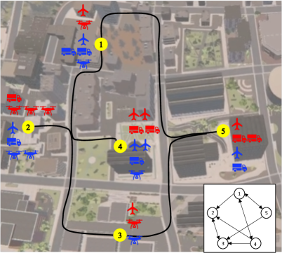
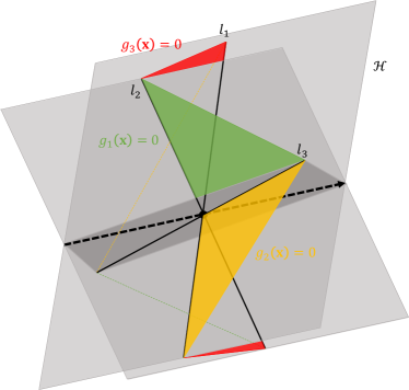
Nevertheless, in addressing the problem of game-theoretic robot allocation, research on the conventional Blotto game exhibits several limitations. First, these studies have mainly focused on unilateral or homogeneous resources [26, 27, 28]. However, the robots can be heterogeneous and have different capabilities, which means the number of robots is not the only criterion of win and loss. Second, considering the environmental constraints and the motion abilities of the robots, there are sites between which no direct routes are accessible, e.g., the aerial robots are not allowed to enter no-fly zones and the wheeled robots may not be able to traverse terrains with sharp hills, tall grass, or mud puddles. Therefore, given these real-world constraints and limitations, the environment in which the robots operate is a non-fully connected graph where robots can transition only between connected sites. However, none of the previous research on resource allocation games involves different types of resources and graph constraints. Therefore, in this paper, we primarily focus on game-theoretic robot allocation on graphs with multiple types of robots (Fig. 1).
First, the game requires both players to allocate robots under graph constraints, i.e., the robots can only be transitioned from one node to the other if there exists an edge between the two nodes. In practical scenarios, the resource allocation among nodes often demands consideration of the relative positions and connectivity of these points, as highlighted by [29, 30], in discussions about offensive and defensive security games. However, [29] mainly focuses on calming the winning conditions for one player in the presence of a more powerful opponent, without computing the equilibrium of the game (i.e., the optimal strategies for the two players). In [30], the main focus is the network security game where the defender places resources to catch the attacker instead of a Colonel Blotto Game. Specifically, we consider distinct nodes to share unidirectional connections. Thus, robots cannot be directly transited between disconnected points. This setting morphs the allocation game into an asymmetric game, detailed further in the subsequent sections.
Second, we consider that both players allocate multiple types of robots that may inhibit each other, termed cyclic dominance (CDH) [31]. In [27] the multiple-resource Colonel Blotto game has been introduced, but it considers different resources to be completely independent of each other. Different from that, For cyclic dominance heterogeneous (CDH) resources, any two types of resources hold a restrictive relationship as in the classic game of Rock-Paper-Scissors. This relationship is widely studied in evolutionary dynamics in biology science. For instance, in [32], Nowak utilized the examples of Uta stansburiana lizard and Escherichia coli to illustrate this mutually restrictive relationship. Similarly, an example of CDH robots could be three types of functional robots—cyber-security robots, network intrusion robots, and combat robots. The cyber-security robot is primarily designed for defensive operations, specializing in counteracting cyber threats. It is equipped with advanced cybersecurity algorithms, enabling it to detect and neutralize attacks from network intrusion robots. The network intrusion robot excels in offensive cyber operations. This robot is capable of executing sophisticated network attacks, targeting vulnerabilities in other robots, particularly those relying on network-based controls such as combat robots. The combat robot is engineered for physical combat and tactical defense. It is armed with state-of-the-art weaponry and robust armor, making it highly effective in direct physical confrontations such as with the cyber-security robot. In other words, a cyber-security robot is capable of defending against network attacks from a network intrusion robot, but it can be physically destroyed by a combat robot. Meanwhile, a network intrusion robot can easily paralyze the network systems of a combat robot, causing it to crash, but it can be defeated by a security robot. In [33], this relationship is represented in matrix form and incorporated into the replicator dynamics. We use the concept of cyclic dominance to distinguish different types of mutual-restrictive robots. Based on it, we formulate a utility function to quantitatively evaluate the outcomes of the game.
We utilize the double oracle algorithm (DOA) to compute the equilibrium of the Colonel Blotto game on graphs. This algorithm was initially proposed by McMahan, Gordon, and Blum [34] and has since been extensively adopted across various domains within game theory. In [35] and [36], DOA was employed to solve two-player zero-sum sequential games with perfect information, with its performance verified on adversarial graph search and simplified variants of Poker. A theoretical guarantee on the convergence of the DOA was also provided. Additionally, Adam [37] employed DOA for the classic Colonel’s Game, juxtaposing it with the fictitious play algorithm and identifying a more rapid convergence rate for the former.
Contributions. We make three main contributions as follows:
-
•
Problem formulation: We formulate a game-theoretic robot allocation problem where two players allocate multiple types of robots on graphs.
-
•
Approach: We leverage the DOA to calculate Nash equilibrium for the games with homogeneous, linear heterogeneous, and CDH robots. Particularly, for the CDH game, we introduce a new transformation rule between different types of robots. Based on it, we design a novel utility function and prove that the utility function is able to rigorously determine the winning conditions of two players. We also linearize the constructed utility function and formulate a mixed integer linear programming problem to solve the best response optimization problem in DOA.
-
•
Results: We demonstrate that players’ strategies computed by our approach converge to the Nash equilibrium and are better than other baseline approaches.
Overall, our main contribution lies in the incorporation of graph constraints into the classical Colonel’s Game and its extension to a heterogeneous context, where the multiple types of robots owned by opposing players are subject to mutual constraints. In addition, we design a novel utility function and utilize the DOA to calculate the equilibrium of this newly formulated game. Furthermore, the simulation results validate that our approach achieves the Nash equilibrium.
II Conventions and Problem Formulation
In this section, we first introduce game-theoretic robot allocation on graphs. The problem can be modeled as a Colonel Blotto game. Then we introduce the Colonel Blotto game including pure and mixed strategies and the equilibrium. Finally, we present the main problems to address in this paper.
II-A Robot Allocation between Two Players on Graphs
The environment where two players allocate robots can be abstracted into a graph as shown in Fig. 1. An ordered pair can be used to define an undirected graph, comprising set of nodes and set of edges . Particularly, a complete graph is a simple undirected graph in which every pair of distinct nodes is connected by a unique edge [38]. Replacing nodes in by ordered sequence of two elements in leads to directed graph, or digraph with a set of edges. For an edge directed from node to , and are called the endpoints of the edge with the tail of and the head of . A directed graph is called unilaterally connected or unilateral if contains a directed path from to or a directed path from to for every pair of nodes [39].
Previous studies on Colonel Blotto games do not incorporate graphs [27, 28, 37]. If the same logic is applied, they can be seen as the games conducted on a complete graph since there is no limitation on the robot transitions between any two nodes. In this paper, we focus on the Colonel Blotto games on unilateral graphs where the robots must be transitioned on the edges. Graph nodes are the strategic points where two players can allocate robots. We denote the number of nodes as . We model the robot allocation by its two characteristics—type denoted as , and number denoted as . If there are robot types i.e., , the number of robots for each type can be denoted by , respectively. In the paper, denotes homogeneous robot allocation and denotes heterogeneous robot allocation. To start the game of robot allocation, there must be an initial robot distribution for both players. Denote and as the initial distribution of -th type robots from Player 1 and Player 2, respectively. Notably, (or ) is a vector of entries, each of which stands for the -th type robots allocated on a particular node. Fig. 2(a) demonstrates an example of homogeneous robot allocation. The initial robot distribution of Player 1 (red) is . Then she translates one robot from node 3 to node 2 and another from node 4 to node 1. The robot distribution becomes . Since , this allocation is valid. Meanwhile, the robot allocation of Player 2 (blue) after one step is . If the rule stipulates that the player who owns more robots on a node wins that node, then the outcome is that Player 2 wins. That is because she wins nodes while Player 1 only wins nodes .
II-B Colonel Blotto Game
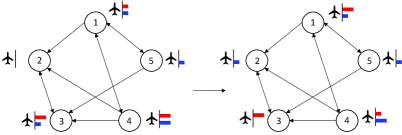
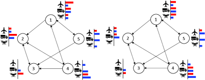
A Colonel Blotto Game is a two-player constant-sum game in which the players are tasked to simultaneously allocate limited resources over several strategic nodes [22]. Each player selects strategies from a nonempty strategy set , where . stands for amount of -th resource allocated on -th node. Each player picks their strategies combination over probability distribution and , respectively. The probability of strategy adopted by Player 1 is denoted as . Analogously for Player 2, it is donated as . This strategy’s combination over the probability distribution is called mixed strategy, denoted by and . The number of strategies in a mixed strategy set is denoted by . For example, if Player 1 decides to apply the mixed strategy of strategies from , then . If , the strategy is called pure strategy. Fig. 2(b) illustrates an example of heterogeneous robot allocation that expands from the case of homogeneous robot allocation (Fig. 2(a)). There are three types of robots, i.e., and each type has five robots, i.e., . There are five nodes in the graph, i.e., . For Player 1,
and for Player 2,
If the probability of taking the first strategy and the second strategy is respectively 0.4 and 0.6, i.e., , then mixed strategy for Player 1 is
While Player 2 takes pure strategy with , thus . Notably, the mixed strategy comprises elements from compact strategy sets and . For each strategy element and , the utility function is a continuous function measuring the outcome of the game for Player 1, while for Player 2 utility function is if the game is zero-sum. In classic Colonel Blotto game (i.e., homogeneous robot allocation), the utility function can be modeled as a sign function since the player allocating more robots to a node wins that node. The utility is the total number of strategic points the player wins, as shown in Equation 1.
| (1) |
Here and are both -dimension vectors since the classic Colonel Blotto game is a homogeneous game where (mentioned in section II-A), and refer to -th entry of and . However, in games with heterogeneous resources, the utility functions can be more complicated.
The triple is called a continuous game. In a continuous game, given two players’ mixed strategies and , expected utility of Player 1 is defined as
Lemma 1
A mixed strategy group is equilibrium of a continuous game if, for all ,
According to [40], every continuous game has at least one equilibrium.
II-C Problem Formulation
We consider a two-player game-theoretic robot allocation on a connected directed graph with . Suppose each player has types of robots with corresponding quantity . The initial robot distributions of the two players are and , respectively. We first introduce two basic assumptions.
Assumption 1 (One-step transition)
We assume the transition of robots between two connected nodes can be accomplished within one step.
Assumption 2 (Perfect information)
We assume the allocation strategies of the two players are public.
With these two assumptions, we aim to compute the equilibrium (i.e., optimal mixed strategies for the two players) for three versions of the game-theoretic robot allocation on graphs.
Problem 1 (Allocation game with homogeneous robots)
All robots are homogeneous (i.e., ). The win or loss at a given node is determined purely by the number of robots allocated. The utility function for the players is introduced in (1), where is a continuous factor ensuring the smoothness and continuity of the function.
Problem 2 (Allocation game with linear heterogeneous robots)
Robots are heterogeneous, i.e., but there exists a linear transformation between different robot types, e.g., with a positive constant.
Problem 3 (Allocation game with CDH robots)
Robots are heterogeneous, i.e., , and they mutually inhibit one another. This is commonly referred to as cyclic dominance [31]. In CDH robot allocation, the number of robots on a node can no longer determine the winning condition of that node since the combination of heterogeneous robots also plays an important role. Therefore new utility function is required to describe this inhibiting relationship, which is introduced in Section IV-C.
III Preliminaries
III-A Double Oracle Algorithm
Input:
-
•
Graph ;
-
•
Continuous game ;
-
•
Initial nonempty strategy set ;
-
•
threshold .
Output:
-
•
-equilibrium mixed strategy set of game ;
The double oracle algorithm was first presented in [34]. Later, it was widely utilized to compute the equilibrium (or mixed strategies) for continuous games. [30, 41]. To better understand the algorithm, we first introduce the notion of best response strategy. The best response strategy of Player 1, given the mixed strategy of Player 2, is defined as
| (2) |
It is Player 1’s best pure strategy against her opponent (i.e., Player 2). Similarly, Player 2’s best response strategy is
| (3) |
The double oracle algorithm begins from an initial strategy set and for the two players, which are picked randomly from strategy space and . is a subgame of , and the equilibrium of this subgame can be calculated by linear programming, as in Algorithm 1, line 2. From the equilibrium of the subgame, notated as and in -th iteration, best response strategies for both players are computed as in Algorithm 1, line 4. If these strategies are not in the subgame strategy set, then add them into the set to form a bigger subgame, and calculate whether equilibrium is reached. According to [37], the equilibrium condition (Lemma 1) is equivalent to the following lemma.
Lemma 2
A mixed strategy group is equilibrium of a continuous game if, for all and ,
| (4) |
is called upper utility of the game, denoted by , and is called lower utility of the game, denoted by . Note that, in practice, (4) is typically replaced by -equilibrium equation for the simplicity of computation.
Therefore, the termination condition is . In addition, since the output is the mixed strategy and too many redundant strategies with a low probability would slow down the algorithm, we delete strategies with a low probability, as shown in Algorithm 1, line 3.
The optimization problem in Algorithm 1, line 2 is a linear programming (LP) problem. Define the utility matrix over and by , with each entry being the utility of Player 1’s -th strategy verses Player 2’s -th strategy, i.e.,
Therefore, the expected utility can be calculated by
Suppose is a matrix (that is, Player 1’s mixed strategy set containing strategies and Player 2’s mixed strategy set containing strategies), the probability distribution of Player 1’s strategies can be calculated by
For Player 2, the probability distribution can be calculated by
These can be solved by linprog in Python.
The most crucial part of the double oracle algorithm is to compute the best response strategy (Algorithm 1, line 4). The graph constraints and various robot types we consider make the computation challenging. First, the strategy set and in (2) and (3) depends on the graph . Given that is unilaterally connected, not all nodes can be reached within one step. Therefore with an initial robot distribution, reachable strategy sets and need to be computed first. This problem was introduced in paper [29], which we briefly summarize in Section III-B. Second, an appropriate utility is essential for computing the best response strategy. However, for CDH robots, no such function exists. To this end, we construct a continuous utility function to handle CDH robots (Section IV-C).
III-B Reachable Strategy Set
We leverage the notion of reachable set for computing strategy sets and on graph . We define the adjacency matrix of a graph as:
The adjacency matrix describes the connectivity of nodes on a graph. We denote the -th type robots distributed on a graph at time by a -dimension vector with the number of nodes and each element the number of this type robots on each node. Then we denote the Transition matrix as
Note that the transition matrix has two characteristics.
-
•
-
•
All valid transition matrices form admissible action space , i.e.,
To to determine closed-form expression of , define extreme action space corresponding to the binomial allocation as
| (5) |
Extreme action space is a finite set and its element forms the base of . Therefore, admissible action space can be calculated as a linear combination of all elements in extreme action space.
Then, given an initial distribution of the -th robot type, , the reachable set for -th robot type can be calculated as
| (6) |
Finally, the strategy set for all types of robots can be expressed as a collection of their individual reachable sets.
| (7) |
The reachable set can be calculated analogously.
IV Approach
In this section, we present solutions to compute the equilibrium (i.e., optimal mixed strategies for the two players) for Problem 1, Problem 2, and Problem 3.
IV-A Approach for Problem 1
In Problem 1, two players allocate homogeneous robots (i.e., ) on graph . We denote initial robot distribution as and , or shorthand and . We first calculate the reachable set of initial strategy sets and by (6) and (7).
| (8) | ||||
Then we utilize the Double Oracle algorithm (Algorithm 1) to compute the optimal mixed strategies for the two players with the utility function introduced in (1). Particularly, assume in -th step is known, the best response strategy for Player 1 is determined by
| (9) |
The approach to solve this problem will be discussed in Section IV-D.
IV-B Approach for Problem 2
In Problem 2, two players allocate linear heterogeneous robots (i.e., ) on graph . Then the strategy space becomes a -dimension matrix. Denote the initial robot distribution as and , which are also -dimension matrices. Different robot types can be linearly transformed, i.e., by an intrinsic matrix , i.e.,
| (10a) | |||
| (10b) | |||
The second equality ensures that the transformation between any two types of robots is reversible and multiplicative. Therefore, all types can be transformed to a specified type , i.e., for all . This means that linear heterogeneous robots are transformed into homogeneous robots. In other words, Problem 2 becomes Problem 1. Specifically, after transformation, strategy space and initial robot distributions become -dimension vectors. Then the reachable set of initial strategy sets and can be calculated by (8) and Problem 2 can be solved using the same approach for Problem 1.
IV-C Approach for Problem 3
In Problem 3, two players allocate cyclic-dominance-heterogeneous (CDH) robots on graph . In this paper, we specify that if robot type dominates robot type , then is capable of neutralizing or overcoming a greater number of than its own quantity. With CDH robots, the linear intrinsic transformation between robot types is broken and not guaranteed to be closed anymore. For example, if and , by circularly converting to , to , and to , the number of increases out of thin air. Therefore, we design a new transformation rule, named elimination transformation between different types of CDH robots.
Elimination transformation. In CDH robot allocation, transformation is valid only when robots can be eliminated but not created between two players. For example, consider , and Player 1 allocates and Player 2 allocates on node . After canceling out the same types of robots, the remaining robot distribution after subtraction on node is . This means Player 1 wins the game since Player 1 can consume Player 2’s at the cost of , and still has one to win node . However, if we transform Player 2’s to , i.e., , the remaining robots are with transformed from , leading to Player 2’s win. This process is wrong because we cannot transform to as we cannot create new type-2 robots out of type-1 robots. Therefore, the robots can only be eliminated but not created. Following this rule, we can transform to cancel out and the remaining can be eliminated by . In the end, we have the remaining robots as , and thus Player 1 wins.
Based on the elimination transformation rule, we construct a novel utility function to decide on the outcome of the game. In particular, we consider three types of CDH robots (i.e., ) as in the case of Rock-Paper-Scissor. 111For , the operation becomes even more complex and differs from the case of , which we explain by an example in the Appendix. We leave the case of for future research. Notably, the inhibiting property of the CDH robot allocation implies that the intrinsic matrix satisfies for .
IV-C1 Construction of outcome interface
Based on the elimination transformation, we first construct an outcome surface that distinguishes between the win and loss of the players, and then design a new utility function of the game in Section IV-C2. The outcome interface defined on is the continuous surface between any two of the three concurrent lines:
| (11a) | ||||
| (11b) | ||||
| (11c) | ||||
Then we formally define the piecewise linear function according to [42, Definition 2.1].
Definition 1 ([42])
Let be a closed convex domain in . A function is said to be piecewise linear if there is a finite family of closed domains such that and if is linear on every domain in . A unique linear function on which coincides with on a given is said to be a component of . Let denote the set of hyperplanes defined by for that have a nonempty intersection with the interior of .
With the definition of the piecewise linear function, we utilize [42, Theorem 4.1] to design our outcome interface, which defines the demarcation between the win and loss.
Theorem 1 ([42])
Let be a piecewise linear function on and be the set of its distinct components. There exist a family of subsets of such that
| (12) |
Conversely, for any family of distinct linear function , the above formula defines a piecewise linear function.
We write the in Max-Min term by Theorem 1. Let be the set of components of on with
| (13a) | ||||
| (13b) | ||||
| (13c) | ||||
where , , and represent the planes constituted by the intersection of in (11b) and in (11c), the intersection of in (11a) and in (11c), and intersection of in (11a) and in (11b), respectively. Let , and , then
| (14) |
Therefore the close form expression of outcome surface is
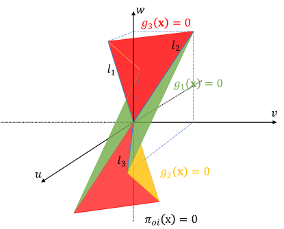
Fig. 3 illustrates and .
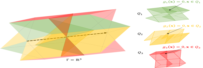
IV-C2 Construction of Utility Function
In this section, we first prove that the outcome surface is the demarcation surface between win and loss. Then we construct the utility function based on the outcome interface. Suppose Player 1 allocates and Player 2 allocates on a node, the robot distribution after subtraction is , , and .
Winning condition. Notably, Player 1 wins on a given node if and only if the remaining robot distribution after subtraction on the node can be elimination transformed into , with and not all of them equal to . Player 2 wins on a given node if and only if the remaining robot distribution after subtraction on the node can be eliminated transformed into , with and not all of them equal to . The game reaches a draw on a given node if and only if the remaining robot distribution after subtraction on the node can be eliminated transformed into , with .
Next, we show the completeness of the winning condition, i.e.,
Theorem 2
222In the appendix, we give an example demonstrating that when the dimension of is larger than 3, no longer belongs to one of these three conditions only., belongs and only belongs to one of the three conditions.
Theorem 2 tells that if can be elimination transformed into with all entries of and , then there is no other different elimination transformation that can transform it into that all entries of . This is obvious since the elimination transformation is a deterministic process in 3D. That is, for a vector ,
-
•
if all entries of are concordant, then by definition can not be eliminated transformed, or can only be eliminated transformed into itself.
-
•
if not all entries of are concordant, we sequentially search through pairs of entries in , specifically the combinations , , and . We select the first pair with different signs to operate an elimination transformation and continue this process until the value of one element in a pair reaches zero. This is a deterministic process and if the newly obtained vector can still undergo an elimination transformation, meaning not all its entries have the same sign. Then we continue this process until we achieve a vector where all entries are concordant. In 3D, this process needs at most two iterations to ensure that the resulting vector has entries of the same sign. Again, each step of this process is deterministic.
Theorem 2 ensures that the defined winning condition divides space into three mutually exclusive subspaces. Indeed, the surface is one of the three subspaces, more precisely, the tie game subspace. corresponding to the Player 1 winning space and corresponding to the Player 2 winning space. That is,
Theorem 3
At a node, Player 1 wins if and only if , Player 2 wins if and only if , and the game is tied if and only if .
Without loss of generality, we prove the winning condition for Player 1. The winning condition for player 2 and the condition for a draw can be proved similarly.
Proof 1
First, we prove the necessity, i.e., if , then Player 1 wins. According to the winning condition, the winning of Player 1 is that can be elimination transformed into , where and not all of them are .
If and not all of them are , then is exactly . If not all , without loss of generality, we assume and and consider three cases below.
-
•
Case 1: , i.e., . In this case, we first transform into until one of them becomes . If is completely eliminated by , or,
(15) then through elimination transformation is transformed into with each entry no less than . If , it means does not suffice to eliminate , and thus we further transform into . If
(16) then suffices to eliminate remaining , and through elimination transformation is transformed into with each entry no less than . Indeed, (16) is valid since
Thus in this case can always be elimination transformation into with entries no less than and not all of them are .
-
•
Case 2: , i.e., . We can still run the transformation process the same as for case 1, but need extra steps to prove (16). Note that (14) reveals an implication of , in face represents the median of and given . Therefore, with , we obtain
(17) Given that and , it is clear that . Thus (17) becomes . Therefore in this case , which shows that (16) is valid.
-
•
Case 3: , i.e., . Based on the proofs of case 1 and case 2, we know that in this case is the median of . is valid as long as holds. Thus we have . With , (15) always holds, which means always suffices to eliminate . Indeed, can be rewritten as
(18) Given , (18) leads to (15). This means can always be eliminated into .
Therefore the necessity is proven.
Then we prove the sufficiency, i.e., if Player 1 wins (or equivalently, can be elimination transformed into with and not all of them being ), then . We consider two cases.
-
•
Case 1: and not all of them are , then is exactly . Obviously, , since the coefficients of piecewise linear function are positive.
-
•
Case 2: Not all , assuming . Upon performing a elimination transformation on , either (15) or (16) must hold since the result invariably ensures that all entries are non-negative. If (15) holds, then , leading to . If (15) does not hold, then (16) must hold and since we have shown that if , then (15) must hold in the proof of necessity. Therefore, either or . If then (16) directly leads to . If , from and (16), we have
(19) Substituting (19) into , we have
Then we have .
Therefore the sufficiency is also proved.
We use an example to further clarify the property of the outcome interface. Suppose the remaining robot distribution after subtraction on a node is . We evaluate this outcome from two views. First, intuitively, Player 2 eliminates all Player 1’s by since , and eliminates all Player 1’s by since , and in the end, Player 2 still has while Player 1 remains nothing. Thus Player 2 wins on this node. In this process, we first convert into , and then convert into , and finally find out that after the transformation there is still remaining on Player 2’s side. The second view is through the outcome surface . Plugging into (14), we have , indicating Player 2 wins. Indeed the calculation of includes three steps. We first compute , i.e., calculating the outcome of converting all types of robots into the , i.e., is . Second, we compute , i.e., calculating the outcome of converting all types of robots into the , which is . Thirdly, we compute , i.e., calculating the outcome of converting all types of robots into the , which is . Finally, we choose the middle value to represent the outcome according to the definition of . This is consistent with the intuition. The reason that the value from the outcome surface is different from that of the intuition is that the plane function , component of , is multiplying the converted term .
The utility function is then computed based on the outcome interface. To ensure function continuity, we assume that Player 1 is only considered to completely win when and the utility for Player 1 is 1. Otherwise, if , Player 1 has an incomplete victory, with their utility being a number that is between 0 and 1. The same applies to Player 2. Note that the direction of the surface’s movement from to is denoted by the black dashed lines in Fig. 3. The illustration of the constructed utility function is shown in Fig. 4.
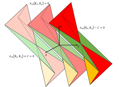
| (20) |
is the threshold for win or loss. The remaining robot distribution after subtraction on -th node is situated on the surface . If , then , indicating an absolute win for Player 1. Conversely, if , then , indicating an absolute win for Player 2. If , then , meaning that one side achieves winning to a certain extent. This way of constructing the utility function ensures its continuity [37], consequently facilitating the calculation of the best response strategy (Algorithm 1, line 4).
IV-D DOA with CDH robots
We next introduce the steps of solving the optimization problem of (9) in Algorithm 1, line 4 with the constructed utility function . The main idea is to rewrite the piecewise linear function into linear inequalities and transform the problem into a linear programming problem.
In (14), has the Max-Min representation. We further rewrite it by linear inequalities. First, we rewrite it as
| (21) |
Note that (21) expresses in the form of linear combination of . To rewrite it into linear inequalities, Lemma 4 is applied. To begin with, we first introduce [37, Lemma C.1] to write the functions in the form of into inequalities form.
Lemma 3 ([37])
Let be a function of , , and . For every such that there is a unique and a possible non-unique solving the system
and it holds .
Based on Lemma 3, one has
Lemma 4
Let be a function of , , and . For every such that there is a unique and a possible non-unique solving the system
| (22) |
and it holds .
Proof 2
, s.t. , there is
where is the solution of the inequality system
and , and is the solution of the inequality system
and , , according to Lemma 3.
Denote as , following . Substituting into the linear inequalities above, we have
Therefore we derive the linear inequalities equivalent to (21) by replacing the operation with (22).
With Lemma 3 and Lemma 4, the optimization problem of (9) can be transformed into mixed integer linear programming (MILP), which can be solved by the optimization solver gurobi [43]. With utility function as , the optimization problem (9) can be reformulated as follows:
Given Player 2’s -th step mixed strategy ,
| (23) |
According to [37, Appendix C], for any , and a constant , there is
or, for simplicity, we can denote as where and . With Lemma 3, we obtain and in the form of linear inequalities system as follows:
where and , , . We can replace the in the linear inequalities as discussed above. Specifically, according to (21), one has
where and , , , for simplicity. Moreover, according to Lemma 4 we can write and into the form of linear inequalities. Finally, the optimization problem in (23) is reformulated into a mixed integer linear optimization problem as follows.
Given Player 2’s -th step mixed strategy ,
with
Note that are linear functions and is bounded. Thus are all bounded. are the large numbers to include their bounds. Since is piecewise linear, both and are bounded and are large number to include their bounds. Besides, since are linear functions, thus all above can be written as .
V Numerical Evaluation
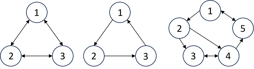
In this section, we conduct numerical simulations to demonstrate the effectiveness of DOA in computing the Nash equilibrium for the robot allocation games with homogeneous, linear heterogeneous, and CDH robots. Following the settings in [20], we use the fraction of the robot population instead of the number of robots to represent the allocation amount. That is, we use to represent the fraction of the population of the -th type of robots allocated on the -th node. Then for the -th robot type. With homogeneous and linear heterogeneous robots, we consider two players to allocate robots on a three-node directed graph with and , i.e., in Fig. 5. For the CDH robot allocation, we consider three robot types as mentioned in Section I, e.g., stands for security robot, stands for network intrusion robot, and stands for combat robot. We evaluate three different cases. In the first case, two players allocate robots on a three-node directed graph with and , i.e., in Fig. 5. In the second case, two players allocate robots on a thee-node directed graph with and , i.e., in Fig. 5. In the third case, two players allocate robots on a five-node directed graph with and , i.e., in Fig. 5.
The initial robot distribution is denoted as for Player 1 and for Player 2. The reachable set and (light blue region in Fig. 8) is calculated based on the extreme action space and as in (5) of Section III-B. The elements of extreme action space can be used to form the boundary of the mixed strategies. The number of elements in extreme action space and are denoted as and , respectively. Then the best response strategy in the DOA (Algorithm 1, line 4) for Player 1 can be calculated by:
| (24) |
| s.t. | |||
We set the outcome threshold in (20) to be for the game with homogeneous and linear heterogeneous robots and for the game with CDH robots. The intrinsic transformation ratios are . The maximum iteration time is set to be 15, and we record 30 trials of the outcome for the following four baselines.
-
•
Baseline 1: Change of one player strategy from the mixed strategy calculated by DOA to the random strategies within constraints. The opponent uses the best response strategy.
-
•
Baseline 2: Change of one player strategy from the mixed strategy calculated by DOA to random strategies within constraints. The opponent uses the best response strategy.
-
•
Baseline 3: Change of one player strategy from the mixed strategy calculated by DOA to random strategies within constraints. The opponent uses the best response strategy.
-
•
Baseline 4: Change of one player strategy from the mixed strategy calculated by DOA to random strategies within constraints. The opponent uses the best response strategy.
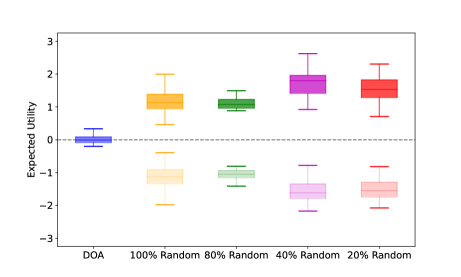
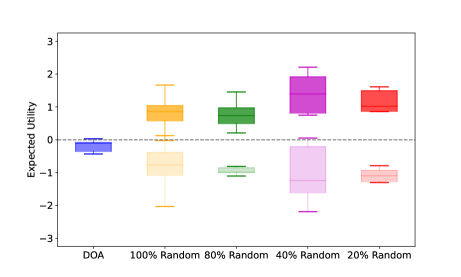
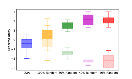
Suppose Player 1’s strategy after change is , we denote the best response strategy of Player 2 for as . According to Lemma 2 [37], any change from the equilibrium strategy of one player will benefit her opponent. This means if we change Player 1’s strategy, then the expected utility tends to decrease from equilibrium value , namely . Particularly, we test two strategy variation schemes. In the first scheme, we adjust Player 2’s strategy according to the baselines and calculate Player 1’s best response strategy. The outcome of this scheme is represented by box plots with a darker shade in Figs. 7, 10, and 11. Conversely, in the second scheme, we modify Player 1’s strategy according to the baselines and calculate Player 2’s best response strategy. Its outcome is represented by box plots with a lighter shade in Figs. 7, 10, and 11.
V-A Homogeneous or Linear Heterogeneous Robots
With homogeneous robots, the utility function in (24) is the classic function (1) introduced in Section II-B. In [37], the allocation game with homogeneous robots has been solved without considering graph constraints. For linear heterogeneous robot allocation, the approach is the same except that we first transform different robot types into one type, as mentioned in Section IV-B. Therefore, we study these two cases together.
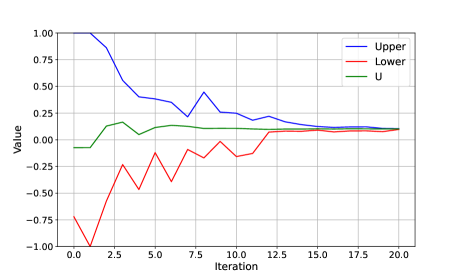
Fig. 6 shows the convergence of DOA, where the blue curve represents the upper utility of the game and the red curve represents the lower utility of the game (Algorithm 1). In iteration 20, their values converge. According to Lemma 2, this demonstrates that the mixed strategies computed by DOA achieve the equilibrium.
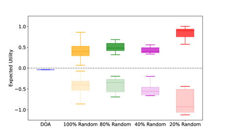
We compare our approach (i.e., DOA) with four baselines across ten trials where we randomly generate the initial allocations for the two players on . Within each trial, we run baselines with randomness involved 1000 times and illustrate them via the box plot. The results are shown Fig. 7. Recall that Lemma 2 states that, in the context of an equilibrium mixed strategy set , any variation in one party’s strategy invariably shifts the outcome towards a direction more advantageous to the opposing party. Here, the utility function is (Section II-B). Thus, a larger benefits Player 1 while a small benefits Player 2. Fig. 7 shows the expected values via the first scheme (i.e., darker shades) are always greater than the value obtained by DOA. That is because, with the first scheme, Player 2’s strategy is randomly changed (with different levels for different baselines). This change benefits Player 1, as reflected by the increase in the game’s expected value. Analogously, the expected values by the second scheme two (i.e., lighter shades) are always less than the value obtained by DOA. Because, with the second scheme, Player 1’s strategy is randomly changed, which benefits Player 2, as reflected by the decrease in the game’s expected value. In other words, any variation from DOA leads to a worse utility of a corresponding player. Therefore, this further demonstrates that the mixed strategies calculated by DOA achieve the equilibrium of the game with homogeneous or linear heterogeneous robots.
V-B CDH Robots
For CDH robot allocation on three-node graphs and , we set the initial robot distribution for Player 1 and for Player 2 as:
For the five-node graph , we set the initial robot distributions as:
The column of refers to different nodes and the row of refers to different robot types. The utility function is in (20).
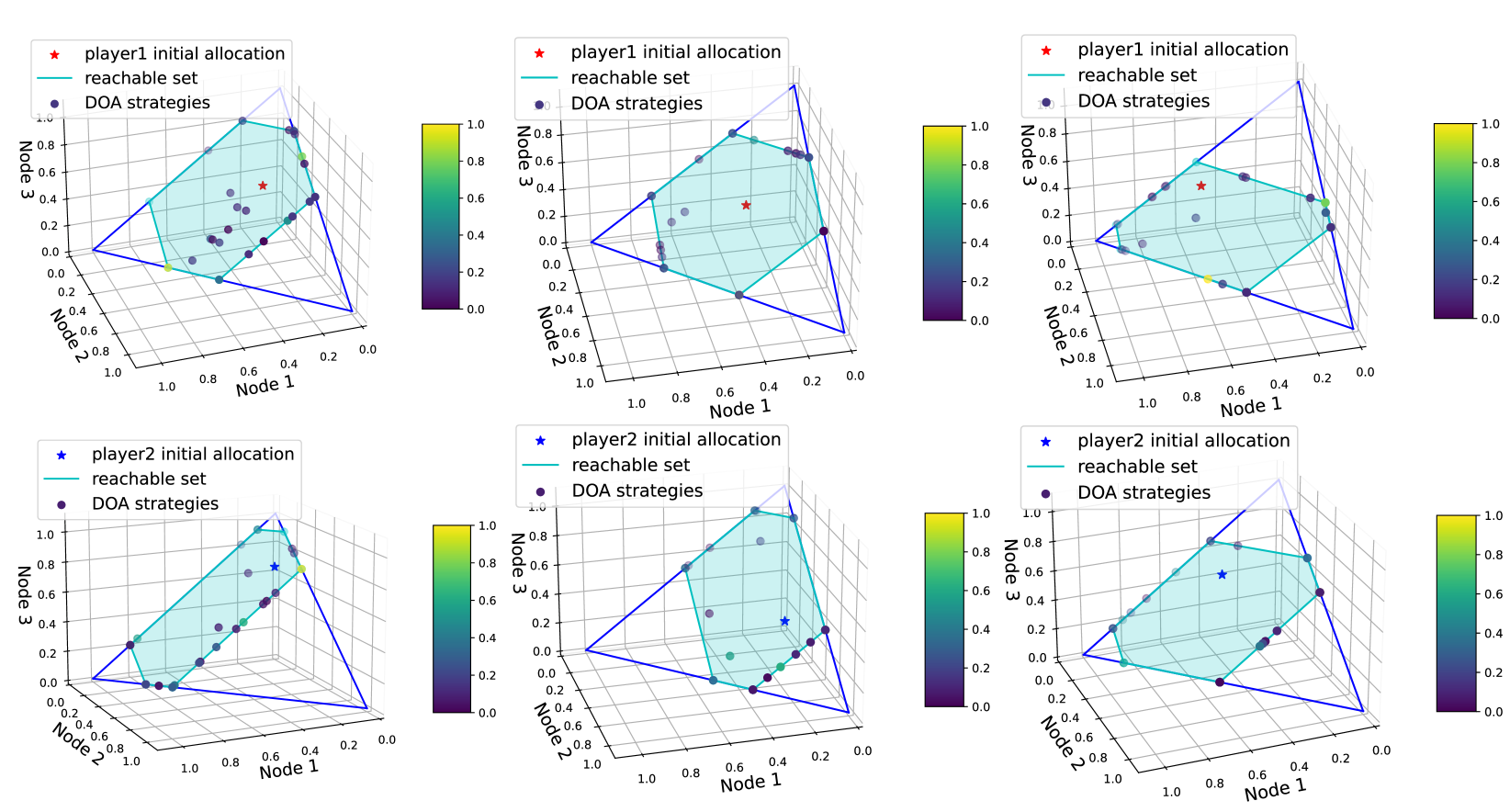
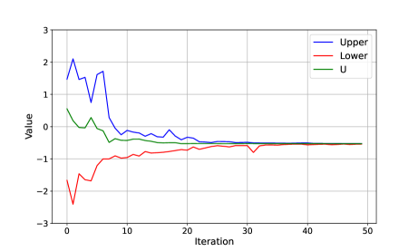
Fig. 8 gives an example of the mixed strategies obtained by DOA. It is observed that for both players the mixed strategies calculated by DOA lie in the reachable set, which illustrates the graph constraints. In Fig. 9 the upper utility of the game (blue curve) and the lower utility of the game (red curve) converge to the expected utility of the game after after 40 iterations. According to Lemma 2, this demonstrates that the mixed strategies computed by DOA are the equilibrium (or optimal) strategies.
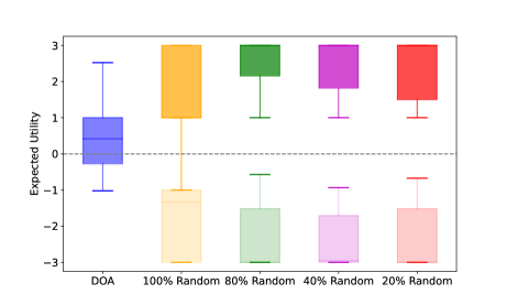
In Fig. 10, we compare the expected utilities by DOA and other baselines (formed via the two schemes) for CDH robot allocation on different graphs , and . Similar to the results of homogeneous robot allocation, the expected utility is nearly zero and any change from the DOA strategies of one player always benefits her opponent, which is in line with the properties of equilibrium (Lemma 2). In Fig. 11, we set the intrinsic transformation ratio as a large number, i.e., to model the case of the absolute dominance heterogeneous robot allocation. The result also aligns with Lemma 2. Therefore, Fig. 10 and Fig. 11 further verify that the mixed strategies calculated by DOA are the equilibrium strategies of the game with the CDH robots.
In Fig. 7, Fig. 10-(b), (c), and Fig. 11, we observe that the value of expected utility calculated by DOA is not zero. Notably, the conventional equi-resource Colonel Blotto game is a zero-sum game [27], [26] and the utility at the equilibrium is zero. This can be demonstrated by Fig. 10-(a) where the two players have the same number of robots and the robots can move flexibly with a complete graph. However, due to the graph constraints in Fig. 7, Fig. 10-(b), (c), and Fig. 11, the game between the two players is not symmetric with different initial robot distributions. This non-symmetry leads to a non-zero utility value at the equilibrium.
VI Conclusions and Future Work
In this paper, we formulated a two-player robot allocation game on graphs. Then we leveraged the DOA to calculate the equilibrium of the games with homogeneous, linear heterogeneous, and CDH robots. Particularly, for CDH robot allocation, we designed a new transformation approach that offers reasonable comparisons between different robot types. Based on that, we designed a novel utility function to quantify the outcome of the game. Finally, we conducted extensive simulations to demonstrate the effectiveness of DOA in finding the Nash equilibrium.
Our first future work is to include the spatial and temporal factors in the robot allocation problem. The current setting assumes instantaneous transitions of robots between nodes. However, in realistic scenarios, spatial and temporal factors such as the distances between nodes and varying transition speeds of the robots need to be considered. Second, we will incorporate the elements of deception into the game, which differs from the current setting that assumes both players to have real-time awareness of each other’s strategy and allocation. This would encourage the players to strategically mislead opponents by sacrificing some immediate gains to achieve larger benefits in the longer term.
References
- [1] B. Zhou, H. Xu, and S. Shen, “Racer: Rapid collaborative exploration with a decentralized multi-uav system,” IEEE Transactions on Robotics, 2023.
- [2] Y. Tao, Y. Wu, B. Li, F. Cladera, A. Zhou, D. Thakur, and V. Kumar, “Seer: Safe efficient exploration for aerial robots using learning to predict information gain,” in 2023 IEEE International Conference on Robotics and Automation (ICRA). IEEE, 2023, pp. 1235–1241.
- [3] A. Ahmadzadeh, J. Keller, G. Pappas, A. Jadbabaie, and V. Kumar, “An optimization-based approach to time-critical cooperative surveillance and coverage with uavs,” in Experimental Robotics: The 10th International Symposium on Experimental Robotics. Springer, 2008, pp. 491–500.
- [4] S. Bhattacharya, R. Ghrist, and V. Kumar, “Multi-robot coverage and exploration on riemannian manifolds with boundaries,” The International Journal of Robotics Research, vol. 33, no. 1, pp. 113–137, 2014.
- [5] R. K. Ramachandran, L. Zhou, J. A. Preiss, and G. S. Sukhatme, “Resilient coverage: Exploring the local-to-global trade-off,” in 2020 IEEE/RSJ International Conference on Intelligent Robots and Systems (IROS). IEEE, 2020, pp. 11 740–11 747.
- [6] V. D. Sharma, L. Zhou, and P. Tokekar, “D2coplan: A differentiable decentralized planner for multi-robot coverage,” in 2023 IEEE International Conference on Robotics and Automation (ICRA). IEEE, 2023, pp. 3425–3431.
- [7] B. Grocholsky, J. Keller, V. Kumar, and G. Pappas, “Cooperative air and ground surveillance,” IEEE Robotics & Automation Magazine, vol. 13, no. 3, pp. 16–25, 2006.
- [8] D. Thakur, M. Likhachev, J. Keller, V. Kumar, V. Dobrokhodov, K. Jones, J. Wurz, and I. Kaminer, “Planning for opportunistic surveillance with multiple robots,” in 2013 IEEE/RSJ International Conference on Intelligent Robots and Systems. IEEE, 2013, pp. 5750–5757.
- [9] P. Dames, P. Tokekar, and V. Kumar, “Detecting, localizing, and tracking an unknown number of moving targets using a team of mobile robots,” The International Journal of Robotics Research, vol. 36, no. 13-14, pp. 1540–1553, 2017.
- [10] L. Zhou and P. Tokekar, “Active target tracking with self-triggered communications in multi-robot teams,” IEEE Transactions on Automation Science and Engineering, vol. 16, no. 3, pp. 1085–1096, 2018.
- [11] L. Zhou, V. Tzoumas, G. J. Pappas, and P. Tokekar, “Resilient active target tracking with multiple robots,” IEEE Robotics and Automation Letters, vol. 4, no. 1, pp. 129–136, 2018.
- [12] L. Zhou and P. Tokekar, “Sensor assignment algorithms to improve observability while tracking targets,” IEEE Transactions on Robotics, vol. 35, no. 5, pp. 1206–1219, 2019.
- [13] S. Mayya, R. K. Ramachandran, L. Zhou, V. Senthil, D. Thakur, G. S. Sukhatme, and V. Kumar, “Adaptive and risk-aware target tracking for robot teams with heterogeneous sensors,” IEEE Robotics and Automation Letters, vol. 7, no. 2, pp. 5615–5622, 2022.
- [14] L. Zhou, V. D. Sharma, Q. Li, A. Prorok, A. Ribeiro, P. Tokekar, and V. Kumar, “Graph neural networks for decentralized multi-robot target tracking,” in 2022 IEEE International Symposium on Safety, Security, and Rescue Robotics (SSRR). IEEE, 2022, pp. 195–202.
- [15] L. Zhou and V. Kumar, “Robust multi-robot active target tracking against sensing and communication attacks,” IEEE Transactions on Robotics, 2023.
- [16] D. B. Reynolds, “Oil exploration game with incomplete information: an experimental study,” Energy Sources, vol. 23, no. 6, pp. 571–578, 2001.
- [17] R. B. Myerson, “Incentives to cultivate favored minorities under alternative electoral systems,” American Political Science Review, vol. 87, no. 4, pp. 856–869, 1993.
- [18] D. Kovenock and B. Roberson, “Coalitional colonel blotto games with application to the economics of alliances,” Journal of Public Economic Theory, vol. 14, no. 4, pp. 653–676, 2012.
- [19] D. Kovenock and B. Roberson, “Conflicts with multiple battlefields,” Oxford Handbooks Online, 2010.
- [20] S. Berman, A. Halász, M. A. Hsieh, and V. Kumar, “Optimized stochastic policies for task allocation in swarms of robots,” IEEE transactions on robotics, vol. 25, no. 4, pp. 927–937, 2009.
- [21] A. Prorok, M. A. Hsieh, and V. Kumar, “The impact of diversity on optimal control policies for heterogeneous robot swarms,” IEEE Transactions on Robotics, vol. 33, no. 2, pp. 346–358, 2017.
- [22] E. Borel, “La théorie du jeu et les équations intégralesa noyau symétrique,” Comptes rendus de l’Académie des Sciences, vol. 173, no. 1304-1308, p. 58, 1921.
- [23] E. Borel, “The theory of play and integral equations with skew symmetric kernels,” Econometrica: journal of the Econometric Society, pp. 97–100, 1953.
- [24] E. Borel, … Applications [de la théorie des probabilités] aux jeux de hasard: cours professé à la Faculté des sciences de Paris. Gauthier-Villars, 1938, vol. 2.
- [25] O. Gross and R. Wagner, A continuous Colonel Blotto game. Rand Corporation, 1950.
- [26] B. Roberson, “The colonel blotto game,” Economic Theory, vol. 29, no. 1, pp. 1–24, 2006.
- [27] S. Behnezhad, S. Dehghani, M. Derakhshan, M. HajiAghayi, and S. Seddighin, “Faster and simpler algorithm for optimal strategies of blotto game,” in Proceedings of the AAAI Conference on Artificial Intelligence, vol. 31, no. 1, 2017.
- [28] A. Ahmadinejad, S. Dehghani, M. Hajiaghayi, B. Lucier, H. Mahini, and S. Seddighin, “From duels to battlefields: Computing equilibria of blotto and other games,” Mathematics of Operations Research, vol. 44, no. 4, pp. 1304–1325, 2019.
- [29] D. Shishika, Y. Guan, M. Dorothy, and V. Kumar, “Dynamic defender-attacker blotto game,” in 2022 American Control Conference (ACC). IEEE, 2022, pp. 4422–4428.
- [30] M. Jain, D. Korzhyk, O. Vaněk, V. Conitzer, M. Pěchouček, and M. Tambe, “A double oracle algorithm for zero-sum security games on graphs,” in The 10th International Conference on Autonomous Agents and Multiagent Systems-Volume 1. Citeseer, 2011, pp. 327–334.
- [31] A. Szolnoki, M. Mobilia, L.-L. Jiang, B. Szczesny, A. M. Rucklidge, and M. Perc, “Cyclic dominance in evolutionary games: a review,” Journal of the Royal Society Interface, vol. 11, no. 100, p. 20140735, 2014.
- [32] M. A. Nowak and K. Sigmund, “Evolutionary dynamics of biological games,” science, vol. 303, no. 5659, pp. 793–799, 2004.
- [33] J. C. Claussen and A. Traulsen, “Cyclic dominance and biodiversity in well-mixed populations,” Physical review letters, vol. 100, no. 5, p. 058104, 2008.
- [34] H. B. McMahan, G. J. Gordon, and A. Blum, “Planning in the presence of cost functions controlled by an adversary,” in Proceedings of the 20th International Conference on Machine Learning (ICML-03), 2003, pp. 536–543.
- [35] B. Bosansky, C. Kiekintveld, V. Lisy, and M. Pechoucek, “Iterative algorithm for solving two-player zero-sum extensive-form games with imperfect information,” in Proceedings of the 20th European Conference on Artificial Intelligence (ECAI), 2012, pp. 193–198.
- [36] B. Bosansky, C. Kiekintveld, V. Lisy, J. Cermak, and M. Pechoucek, “Double-oracle algorithm for computing an exact nash equilibrium in zero-sum extensive-form games,” in Proceedings of the 2013 international conference on Autonomous agents and multi-agent systems, 2013, pp. 335–342.
- [37] L. Adam, R. Horčík, T. Kasl, and T. Kroupa, “Double oracle algorithm for computing equilibria in continuous games,” in Proceedings of the AAAI Conference on Artificial Intelligence, vol. 35, no. 6, 2021, pp. 5070–5077.
- [38] J. Bang-Jensen and G. Gutin, “Basic terminology, notation and results,” Classes of Directed Graphs, pp. 1–34, 2018.
- [39] J. Gómez, E. A. Canale, and X. Muñoz, “Unilaterally connected large digraphs and generalized cycles,” Networks: An International Journal, vol. 42, no. 4, pp. 181–188, 2003.
- [40] I. L. Glicksberg, “A further generalization of the kakutani fixed theorem, with application to nash equilibrium points,” Proceedings of the American Mathematical Society, vol. 3, no. 1, pp. 170–174, 1952.
- [41] B. Bosansky, C. Kiekintveld, V. Lisy, and M. Pechoucek, “An exact double-oracle algorithm for zero-sum extensive-form games with imperfect information,” Journal of Artificial Intelligence Research, vol. 51, pp. 829–866, 2014.
- [42] S. Ovchinnikov, “Max-min representation of piecewise linear functions,” arXiv preprint math/0009026, 2000.
- [43] Gurobi Optimization, LLC, “Gurobi Optimizer Reference Manual,” 2023. [Online]. Available: https://www.gurobi.com
We use an example to explain the hardness caused by increasing the number of robot types to four, i.e., . Suppose there are four types of robots , and the intrinsic matrix is
Note that the entries (denoted as in the intrinsic matrix) are not defined, as they are not involved in the calculation. For instance, on a node, Player 1’s allocation is while Player 2’s allocation is . Therefore the remaining robot distribution after subtraction is . This scenario presents a challenging outcome to determine a clear winner. Consider the intrinsic relationship between and and that between and . Given that equals , the elimination of from results in a remaining balance of . Similarly, the elimination of from leads to a balance of . From the perspective of the remaining robots, represented as , it shows that Player 1 wins. However, if we instead consider the countering relationship between and and that between and . Following the same logic, the outcome becomes , showing Player 2 is the winner. It is important to notice that both approaches adhere to the elimination transformation rule in Section IV-C. This dichotomy shows the complexity and ambiguity in adjudicating a definitive winner in this context. This implies that in the case of , it is necessary to introduce new mechanisms for determining win or loss on each node.
Notably, the intrinsic matrix in the above example is not deliberately constructed. In fact, any intrinsic matrix that reflects the CDH relationships between different robot types will inevitably lead to such issues. In Section IV-C2, we prove that for , outcome interface is the demarcation surface of win and loss. However, the winning condition described in Section IV-C does not hold for , and thus the demarcation surface does not hold either. We conjecture that the demarcation for is a polytope, which we leave for future study.