Double Hopf bifurcation in nonlocal reaction-diffusion systems with spatial average kernel111This research is supported by National Natural Science Foundation of China (No 11771109).
Abstract
In this paper, we consider a general reaction-diffusion system with nonlocal effects and Neumann boundary conditions, where a spatial average kernel is chosen to be the nonlocal kernel. By virtue of the center manifold reduction technique and normal form theory, we present a new algorithm for computing normal forms associated with the codimension-two double Hopf bifurcation of nonlocal reaction-diffusion equations. The theoretical results are applied to a predator-prey model, and complex dynamic behaviors such as spatially nonhomogeneous periodic oscillations and spatially nonhomogeneous quasi-periodic oscillations could occur.
Keywords : reaction-diffusion system; double Hopf bifurcation; nonlocal effect; normal forms.
1 Introduction
Reaction-diffusion equations have been proposed to model the complex phenomenon in cell biology, neural network, virus dynamics, biochemical reaction, etc., see [35, 52] and references therein. However, individuals of a species at different locations may compete for common resource or communicate by chemical means [7, 16, 21], and nonlocal interactions should be considered. In 1989, Britton [7] proposed a single population model with nonlocal effect, where the nonlocal term takes the following form:
| (1.1) |
Here is the region where the population lives, represents the density of the species at location and time . The model is based on the following two assumptions:
-
(i)
individuals in grouping together can reduce the risk of predation, which is referred to as the aggregation mechanism;
-
(ii)
the intraspecific competition at a certain point depends on not only the density at this point but also a weighted average in the neighborhood of this point.
For unbounded one spatial dimension domain , Britton [7] also considered the nonlocal effects on two species competition model, and it was shown that the aggregation may lead to the coexistence of the two species. For bounded domain , a typical scenario of nonlocal dispersal is the “spatial average kernel”, that is,
| (1.2) |
Furter and Grinfeld [21] obtained that this average kernel can induce spatial nonhomogeneous patterns even for single population model, see [51] for more general models.
There have been extensive results on the nonlocal effects, including existence and stability of solutions, traveling wave solutions, pattern formation, bifurcation analysis, etc., see [5, 6, 22, 24, 17, 38, 16, 20, 23, 43, 10, 12, 13, 11] and references therein. For unbounded one spatial dimension domain , Merchant and Nagata [43] chose different types of kernel , and showed that the nonlocal competition could induce complex spatiotemporal patterns, see also [3, 49]. Motivated by [43], Chen et al. [13, 11] considered the case that the spatial domain , and chose the spatial average kernel, i.e., . They found that, for the nonlocal Rosenzweig-MacArthur (RM) and Holling-Tanner predator-prey models, the constant positive steady state could lose the stability when the given parameter passes through some Hopf bifurcation values, and the bifurcating periodic solutions near such values can be spatially nonhomogeneous. It is well known that Hopf bifurcation has been used to illustrate the periodic phenomena in the natural world, such as regular changes in population size, the periodic outbreak of infectious diseases, and chemical oscillations of some autocatalytic reactions [32, 44, 31]. However, for reaction-diffusion system without nonlocal effect, the bifurcating periodic solutions near the threshold are always spatially homogeneous, while nonhomogeneous periodic solutions can also occur through Hopf bifurcation, but they are always unstable, and consequently hard to simulate. Note that, nonlocal effect could also induced spatially nonhomogeneous steady states through steady state bifurcation[21, 51]. Therefore, nonlocal effect could be used as a new mechanism for pattern formation.
We point out that, for reaction-diffusion equations with nonlocal delay effect, the Hopf bifurcation has also been studied by many researchers, see [10, 12, 29, 30, 28, 55, 56, 25, 26] and references therein. For the homogeneous Neumann boundary condition, Gourley and So [25] showed the existence of Hopf bifurcation for a food-limited population model, see also [38] for the model with age structure. For the homogeneous Dirichlet boundary condition, Chen and Shi [10] developed the method proposed by Busenberg and Huang [9], and studied the existence of Hopf bifurcation near the positive spatially nonhomogeneous steady state. Different from [9, 10], Guo [29] proposed the method of Lyapunov-Schmidt reduction to show the existence and even the multiplicity of the spatially nonhomogeneous steady state, and the associated Hopf bifurcation. There are also other results on Hopf bifurcation for reaction-diffusion models with nonlocal delay, see e.g. [26, 33, 55].
The above mentioned steady state and Hopf bifurcations are both codimension-one bifucation. A natural question is that whether nonlocal effect could induce codimension-two bifurcation for reaction-diffusion equations. For the reaction-diffusion equation, the interaction of a Turing instability (leading to spatially nonhomogeneous steady states) with a Hopf bifurcation (giving rise to temporal oscillations) has been observed and studied in chemical, biological and physical systems, see [42, 41, 57, 48] and references therein. For example, Rovinsky and Menzinger [48] studied this Turing-Hopf interaction for three models of chemically active media by using Poincaré-Birkhoff method and shown the bistability of spatially nonhomogeneous steady states and homogeneous oscillations. In the framework of amplitude equation formalism, De Wit et al. [57] investigated the bifurcation scenarios near the Turing-Hopf singularity. Recently, to show an accurate dynamic classification at this singularity, Song et al.[54] applied the normal form theory proposed by Faria [18] to a general reaction-diffusion equation, and obtained a series of explicit formulas for calculating the normal forms associated with the Turing-Hopf bifurcation. This spatiotemporal dynamics induced by the Turing-Hopf bifurcation were observed in several reaction-diffusion models [53, 59, 4], see also [1, 50] for the reaction-diffusion system with delay. Another typical codimension-two bifurcation is the double Hopf bifurcation. As in the Turing-Hopf bifurcation, when the parameters vary near the threshold value, the system may exhibit rich dynamics such as periodic orbit, invariant two torus, invariant three-torus, and even chaos, see e.g. [27, 45, 15, 34, 37, 60]. Recently, for a general delayed reaction-diffusion system with time delay, Du et al. [15] also obtained an algorithm for deriving the normal form near a codimension-two double Hopf bifurcation by virtue of the the normal form method proposed by Faria [19, 18].
To our knowledge, compared to the classical reaction-diffusion system, few studies have considered the high codimensional bifurcations in nonlocal reaction-diffusion systems. Recently, Wu and Song [58] studied the dynamical classification of a nonlocal diffusive Rosenzweig-MacArthur model near the Turing-Hopf singularity. A numerical simulation [13] revealed that two Hopf bifurcation curves could intersect in a two-parameter plane. However, there exist no results on double Hopf bifurcation for nonlocal reaction-diffusion systems. In this paper, we aim to consider this problem, and consider the following general reaction-diffusion system
| (1.3) |
where with and , , with , , with is smooth, and . We point out that if , then system (1.3) is reduced to a general form in [21]. If , then (1.3) becomes a two-component interaction system, which could model the nonlocal intraspecific and interspecific competition for population models, see [43, 2, 3, 49]. The purpose of this paper is to develop an explicit algorithm for computing normal forms on the center manifold near a codimension-two double-Hopf singularity for model (1.3). We should remark that when the ratio of two angular frequencies is some particular value, e.g. 1:2, the corresponding double-Hopf bifurcation may be codimension-three, referred to as the strong resonance case. In this article, we will not consider this case and focus only the codimension-two double Hopf bifurcation. We find that, compared with the traditional reaction-diffusion system, (1.3) is more likely to induce spatial nonhomogeneous patterns, and consequently exhibit rich dynamical behaviors at the corresponding singularity, such as spatially nonhomogeneous periodic solutions, spatially nonhomogeneous quasi-periodic solutions, coexistence of homogeneous/nonhomogeneous oscillations, and so on.
We also adopt the framework of [18] to compute the normal forms on the center manifold of system (1.3) at the codimension-two double Hopf singularity. In summary, we first rewrite system (1.3) into an abstract form, and by decomposing the phase space into center subspace and its complementary space, we obtain the equivalent system on the center manifold. Then a recursive transformation of variables is used to derive the four-dimensional normal forms. During this process, we construct a Boolean function to deal with the impact of nonlocal terms on the computation, which is the innovation. Particularly, for the case of , we list some additional formulas in Appendix A which could help to obtain all the coefficient vectors that appear in the process of computing normal forms.
The rest of the paper is organized as follows. The decomposition of phase space and some preliminaries are given in Section 2. The computation of normal forms associated with the codimension-two double Hopf bifurcation is presented in Section 3. In Section 4, we apply our theoretical results in Section 3 to a diffusive Holling-Tanner system with spatial average kernel in prey and obtain the normal forms near the duoble-Hopf singularity. Some periodic oscillations and quasi-periodic quasi-periodic oscillations are also derived numerically in this section. Finally, we give some discussion and conclusion for this paper, and in the Appendix, we collect the details of the coefficient vectors that appear in Section 3 when . Throughout the paper, we denote by the set of positive integers, and the set of non-negative integers.
2 Decomposition of the phase space
In this section, we adopt the framework of [18] to compute the normal forms of the double Hopf bifurcation. To use the center manifold theory for reduction[39, 27, 32], we need rewrite system (1.3) into an abstract form and decompose the phase space.
We first define the following real-value Sobolev space
and then the linear map is smooth from to . Denote
It follows from Appendix C of [32] that is also smooth from to . Hence, system (1.3) can be written as the following abstract form
| (2.1) |
where
Let
| (2.2) |
where stands for the Fréchet derivative of with respect to at . To figure out the double Hopf bifurcation with two pairs of purely imaginary eigenvalues, we define the following complexification space of :
with the complex-valued inner product , defined by
where , .
Considering the perturbation caused by the nonlocal terms, we rewrite system (2.1) in a intuitive form
| (2.3) |
where and are bounded linear operators from to , and is a function such that and .
Then the linearization of system (2.3) at takes the following form
| (2.4) |
It is well known that the eigenvalue problem
has eigenvalues (), and the corresponding normalized eigenfunctions
| (2.5) |
Letting , , where is the th unit coordinate vector of , we see that are eigenfunctions of with corresponding eigenvalues , and form an orthonormal basis of .
For and , we define , and denote
Let
be the eigenfunction with respect to eigenvalue . Then
| (2.6) |
where . Note that
| (2.7) |
Then (2.6) is equivalent to a sequence of characteristic equations:
| (2.8) |
To consider the double Hopf bifurcation, we assume that there exists such that the following conditions hold:
-
Assume that for and , i.e., we only consider the codimension-two double Hopf bifurcation of non-resonance and weak resonance instead of the codimension-three of strongly resonant case.
-
The conjugate eigenvalues are obtained by (2.8), and the corresponding eigenvalues belong to for . Without lose of generality, we assume .
Let , where , and then (2.3) can be transformed as
| (2.9) |
where , , , and . Then the linear system of (2.9) on is equivalent to the following ODEs on :
| (2.10) |
where is an matrix, and
Denote by the formal adjoint of under the scalar product on :
Let and let
be the basis of the generalized eigenspace of and corresponding to the eigenvalues , respectively. Then
| (2.11) |
where , , and is an identity matrix. Then we can decompose the phase space :
| (2.12) |
where , and is the projection, defined by
Therefore, can be rewritten in the following form:
| (2.13) |
where , , , and . For simplification of notations, we denote and
| (2.14) |
In the following, we will also use the symbol instead of . Now system (2.9) is equivalent to the following abstract ODEs in
| (2.15) |
where , , and is the restriction of on .
3 Center manifold reduction and normal forms for double Hopf bifurcation
3.1 Center manifold reduction
Consider the formal Taylor expansions
where is the th Fréchet derivation of . Then system (2.15) can be rewritten as
| (3.1) |
where , and is defined by
| (3.2) |
with .
It follows from [18] (see also [14]) that the normal forms of (3.1) can be obtained by a recursive transformation of variables
with . Here, for a normed space , we denote be the space of homogeneous polynomials of degree in variables , with coefficients in , that is,
| (3.3) |
where , , , , , and the norm is defined as the sum of the norms of the coefficients .
We denote by the terms of order obtained after the computation of normal forms in the preceding steps, and define the operators by
| (3.4) |
With the recursive procedure and dropping the tilde for simplicity of notations, (3.1) becomes
| (3.5) |
where , are the new terms of order and given by
Here, can be computed by
| (3.6) |
where is the inverse of with range defined on , is the projection operator associated with the preceding decomposition of over .
3.2 Normal forms up to second order
By (3.4) and assumption , it is easy to verify that
| (3.7) |
Here is the th unit coordinate vector of , and are defined as in (3.3). Therefore,
| (3.8) |
Hence, the normal forms up to second order of (2.1) on the center manifold of the origin near has the form
| (3.9) |
with .
To show the specific expressions of , we consider the Taylor expansions of , and :
Therefore, the second order term of is
| (3.10) |
Recalling that , and , we have . Plug (2.13) into (3.10) at , and then becomes
where with is defined as in (2.13). By (3.2), we have
| (3.11) |
To write (3.11) explicitly, we define the following Boolean function
| (3.12) |
3.3 Normal forms up to third order
From (3.7), we have
| (3.15) |
According to (3.5), the normal forms up to third order has the form
where . The new third order can be calculated by
| (3.16) |
where are given as in (3.6), and . It follows from (3.13) that , and we still have to calculate the following four parts:
which will be shown in the following.
(a) The computation of
.
The third order Fréchet derivative of at is
where , , is the coefficient vector of . Then we have
Thus,
| (3.17) |
where
with , and
(b) The computation of
.
(c) The computation of and
.
Recalling from (3.10) that and by virtue of (3.18), we have
| (3.22) |
where , and
| (3.23) |
with and are linear operators from to , defined by
| (3.24) |
Here, , are coefficient vectors. By (3.22), we can easily obtain
Let with
Then we have
and
where . According to (3.15), we only need to calculate the following types of for some :
and the following discussion is divided into three cases:
Clearly,
Then
and
Therefore, we have
where
Now, we compute the . From (3.4), we have
which leads to
| (3.25) |
where is the Booean function defined as in (3.12).
In addition, by (3.2), we have
| (3.26) |
which, together with the fact
| (3.27) |
yields
| (3.28) |
Substituting (3.25) and (3.26) into (3.28) and balancing power of coefficients for in (3.28) gives
By the fact
we have
and
Therefore, we obtain
where
Using the same method as the one in , we can obtain
.
In fact, we have
Then
and
Hence, we obtain
where
With the same method mentioned in , we have
Now, we obtain the full expression of :
| (3.29) |
where
Then, by (3.14) and (3.29), the normal forms for double Hopf bifurcation up to the third order take:
| (3.30) |
and by virtue of the polar coordinate transformation and variable substitution:
the system (3.30), truncated at the third order, becomes
| (3.31) |
where
Clearly, is always an equilibrium and that up to three other non-negative equilibria solutions can appear:
The dynamics of system (1.3) near the double Hopf bifurcation point is topologically equivalent to that of (3.31) near . Here is associated with the positive constant steady state, is associated with the spatially homogeneous periodic solution, is associated with the spatially nonhomogeneous periodic solution, and is associated with the spatially nonhomogeneous quasi-periodic solution. Moreover, according to [27] there are twelve distinct types of unfoldings according to the signs of coefficients , , and (see Table 1).
| Case | Ia | Ib | II | III | IVa | IVb | V | VIa | VIb | VIIa | VIIb | VIII |
|---|---|---|---|---|---|---|---|---|---|---|---|---|
| +1 | +1 | +1 | +1 | +1 | +1 | –1 | –1 | –1 | –1 | –1 | –1 | |
| + | + | + | – | – | – | + | + | + | – | – | – | |
| + | + | – | + | – | – | + | – | – | + | + | – | |
| + | – | + | + | + | – | – | + | – | + | – | – |
Remark 3.1.
The expressions presented to calculate the normal forms seem complicated and tedious, and some very important coefficient vectors are not explicitly shown, for example, , , , . For an abstract equation with a large number of variables, it may take a lot of work to express all these coefficient vectors, but if the system is only of two variables, i.e., , this complexity can be reduced. We could give the explicit representation of these coefficient vectors by partial derivatives of and the basis of center subspace, and we put this in Appendix.
4 Applicaton to a predator-prey model
In this section, we consider the following reaction-diffusion Holling-Tanner system with nonlocal prey competition:
| (4.1) |
where , and represent the prey and predator densities at location and time respectively, stands for the nonlocal prey competition, and are parameters and all positive. Particularly, is the intrinsic growth rate of predator, and are the diffusive rates, and and measure the strength of interspecific and intraspecific interaction.
The model (4.1) was first proposed and discussed by Merchant and Nagata [43] when and their results indicate that the nonlocal competition may be an important mechanism for pattern formation. When , Chen et al.[11] studied the existence of spatially nonhomogeneous periodic solutions induced by nonlocal competition. When , the model (4.1) is reduced to the classical Holling -Tanner predator-prey model, of which the dynamics have been extensively studied (see e.g. [10, 40, 47, 46, 36] and references therein). It’s worth mentioning that (4.1) is more likely to undergoes a Hopf bifurcation than the classical Holling-Tanner system [11, 36], which increases the possibility for double Hopf bifurcation.
The system (4.1) has a unique constant positive equilibrium with satisfying , and is strictly decreasing with respect to . Therefore, we could choose as one parameter instead of and apply the method obtained in previous sections to compute the normal forms of system (4.1) near the double Hopf singularity.
4.1 Linear analysis and existence of double Hopf bifurcation
Let , and then the linearized system of model (4.1) at the positive equilibrium has the form
where , and
The sequence of characteristic equations are as follows
| (4.2) |
where
| (4.3) |
and for ,
| (4.4) |
For simplicity of notations, we denote
| (4.5) |
The following lemma is a summary of the properties on (4.5), and the proof is trivial and we omit it.
Lemma 4.1.
Suppose that , , and are defined in (4.5).
-
1.
If , then for all . Moreover, there exists such that , for , and for .
-
2.
Let . Then , for , and . for .
-
3.
If , then there exists such that , for , and for . Moreover, for , and for .
The existence of spatially nonhomogeneous Hopf bifurcation was studied by Chen et al. in [11], here we state the main results below without proof.
Theorem 4.2.
[Theorem 2, [11]] Suppose that , , and define
| (4.6) |
where , are defined as Eq.(4.5) and Lemma 4.1. Then the following two statements are true.
-
If , or but , then is locally asymptotically stable for .
-
If and , then there exist two sequences and , , such that
(4.7) and these points satisfy
(4.8) where is defined as in Eq.(4.4), such that is locally asymptotically stable for and unstable for . Moreover, system (4.1) undergoes Hopf bifurcation at when , , and the bifurcation periodic solutions near are spatially nonhomogeneous.
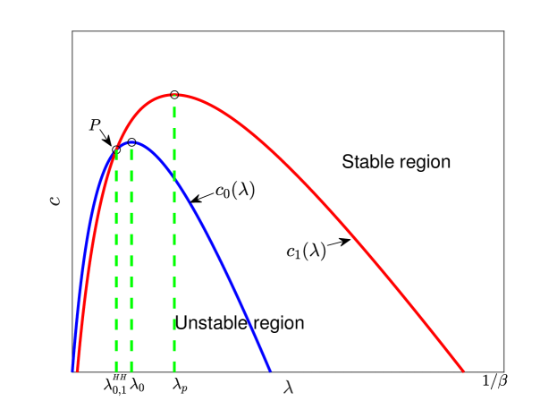
Theorem 4.3.
Note that, if , the large scale is always accompanied by nonhomogeneous Hopf bifurcation, but the corresponding branch curve will not intersect in the parameter plane. Therefore, the double Hopf point can only be the interaction of spatially homogeneous and nonhomogeneous Hopf branches. Hence we consider the case
In this premise, we can restrict the parameter space to a rectangular region, namely,
| (4.9) |
and for fixed , there exist two points , such that
| (4.10) |
Then we have the following result.
Theorem 4.4.
Let with , . Then the following statements hold.
-
If , then the positive steady state is locally asymptotically stable when and unstable when , where is defined as in (4.9), and is defined by
(4.11) where , .
Proof.
Denote , namely,
| (4.13) |
Clearly, , and if , then for any and . Note that , and , hence we have
It is easy to verify that when .
If , then for any and , which means that . Thus, we have that the stable region is exactly , which proves .
If , then , and consequently, there exists a positive integer
| (4.14) |
such that maximally equals to zero. Consequently for , we have , which together with the fact yields that there exists a such that . The critical point can be represented explicitly by
| (4.15) |
Since when and , when , we can give the representation of the stable region in the plane as follows
which is equivalent to . ∎
Remark 4.5.
Remark 4.6.
If , then Turing bifurcation or even Turing-Hopf bifurcation may occur under some conditions, the boundary of stable region will become more complex and the system may exhibit rich dynamics near the Turing-Hopf bifurcation point. If the parameters are chosen properly, the coexistence of the spatially nonhomogeneous periodic solutions and spatially nonhomogeneous steady states can be observed [1, 50, 53].
4.2 Normal forms for double Hopf bifurcation
It follows from Theorem 4.4 that if and , then the spatially homogeneous Hopf bifurcation and spatially nonhomogeneous Hopf bifurcation may occur simultaneously. In this section, we shall calculate the normal forms on the center manifold to investigate the dynamics of system (4.1) near the possible double-Hopf bifurcation singularity .
Let , and with , , then system (4.1) becomes
| (4.16) |
Consider the Taylor expansion
where , , and
| (4.17) |
Then Eq.(4.16) can be rewritten as
| (4.18) |
where
| (4.19) |
It follows from Section 2 that and its adjoint have two pairs of purely imaginary roots and with
| (4.20) |
and other eigenvalues have negative real parts.
Denote and the eigenfunctions of and its dual relative to with , such that
where is defined as in (2.5). Specifically, we let , and after a direct calculation, we have
| (4.21) |
Noticing that and , then from (3.13) and (3.14), we have
| (4.22) |
Applying the method given in Appendix, we obtain
| (4.23) |
and
| (4.24) |
where . The coefficient vectors required in are given by
| (4.25) |
Other formulas appearing in the process of computing normal forms can be obtained from the above formulas.
4.3 Numerical simulations
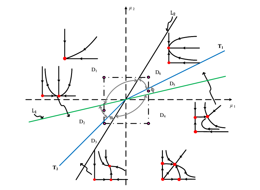
In this section, we give some simulations to support our theoretical results. The dynamic classification near the double Hopf bifurcation point is presented by applying the normal form method, and a particular bifurcation diagram and corresponding phase portraits are shown in Fig. 2.
Take
It follows from Theorem 4.4 and Eq.(4.5), the double Hopf bifurcation point . Note that , then using the formulas (3.30), (3.31) and algorithm (4.22)(4.25), we have
According to the classification for planar vector field in [27], Case occurs, and we can divide the plane into six dynamic regions with
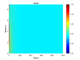
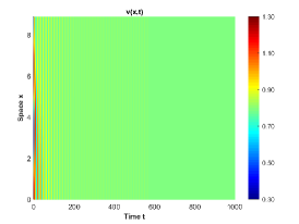
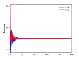
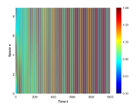
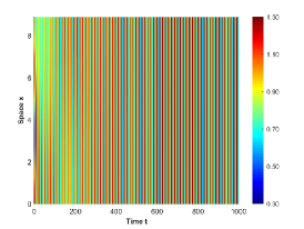
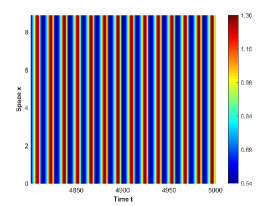
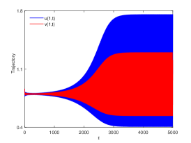
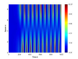
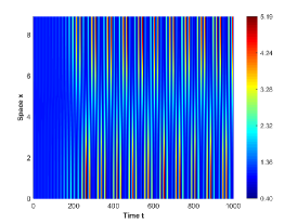
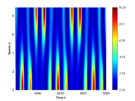
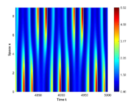
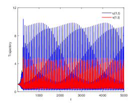
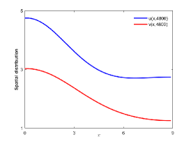
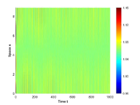
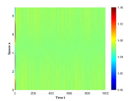
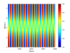
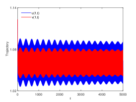
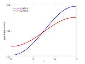
There are four possible attractors in Fig. 2: spatially homogeneous steady state, spatially homogeneous periodic solution, spatially nonhomogeneous periodic solution and spatially nonhomogeneous quasi-periodic solution. In the following, we give a detailed numerical simulation for these attractors, see Fig. 3 Fig. 6.
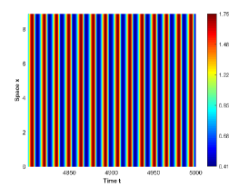
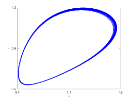
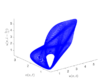
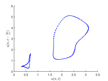
We remark that when , there exists a stable spatially nonhomogeneous quasi-periodic solution, and this quasi-periodicity is not easily seen in Fig. 5. Then we present it on a Poincaré section. Fix , we choose the solution curve and Poincaré section , and the results are shown in Fig. 7 in which we can see that system has a quasi-periodic solution on a 2-torus. Here we only present the case in region , since and are similar. We mention that the spatially nonhomogeneous periodic solution and quasi-periodic solution are new spatiotemporal dynamic behaviors compared to the original system without nonlocal terms. This shows that nonlocal terms can enrich the dynamic behaviors of the system.

5 Discussion and conclusion
In this paper, we develop an algorithm for computing normal forms associated with the codimension-two double Hopf bifurcation for a general reaction-diffusion system with spatial average nonlocal kernel and Neumann boundary conditions. The algorithm looks complicated, but it is actually easy for computer implementation, especially when the system consists of only two variables. We introduce a Boolean function to handle the effects of nonlocal terms on the computation of normal forms. The system can exhibit rich dynamics near the double Hopf bifurcation singularity, and the possible attractors near this degenerated point mainly include spatially homogeneous/nonhomogeneous periodic solutions, spatially nonhomogeneous quasi-periodic solutions.
We apply our result to a reaction-diffusion Holling-Tanner system with nonlocal prey competition. The qualitative analysis reveals that the dynamic behaviors of the system with nonlocal terms is more complex than that of the original system. The unfolding of (see Table.1) occurs in our numerical simulations, and the spatially homogeneous and nonhomogeneous periodic solutions are observed from numerical simulations. Furthermore, The existence of the spatially nonhomogeneous quasi-periodic solution is verified in Poincaré section.
Appendix A Appendix
This appendix is an extension of the case that , and we shall show the details of the coefficient vectors that appear in Section 3. Without loss of generality, we denote
with , . Note that , i.e., , then for , we have
Then the coefficient vectors , , shown in section 3 can be obtained by computing the following partial derivatives, where , and other symbols are similarly defined:
and
The coefficient vectors required in are given by
and those in are as follows:
References
- [1] An, Q. & Jiang, W. [2018] “Spatiotemporal attractors generated by the Turing-Hopf bifurcation in a time-delayed reaction-diffusion system”, Discrete Contin. Dyn. Syst. Ser. B, https://doi.org/10.3934/dcdsb.2018183 (2018)
- [2] Banerjee, M. & Volpert, V. [2016] “Prey-predator model with a nonlocal consumption of prey”, Chaos, 26, 083120.
- [3] Banerjee, M. & Volpert, V. [2017] “Spatio-temporal pattern formation in Rosenzweig–MacArthur model: Effect of nonlocal interactions”, Ecological complexity, 30, 2-10.
- [4] Baurmann, M., Gross, T. & Feudel, U. [2007] “Instabilities in spatially extended predator-prey systems: Spatio-temporal patterns in the neighborhood of Turing-Hopf bifurcations”, J. Math. Biol., 245, 220-229.
- [5] Berestycki, H., Nadin, G., Perthame, B. & Ryzhik, L. [2009] “ The non-local Fisher-KPP equation: travelling waves and steady states”, Nonlinearity, 22, 2813–2844.
- [6] Billingham, J. [2003] “ Dynamics of a strongly nonlocal reaction-diffusion population model”, Nonlinearity, 17, 313–346.
- [7] Britton, N. F. [1989] “ Aggregation and the competitive exclusion principle”, J. Theor. Biol., 136, 57–66.
- [8] Britton, N. F. [1990] “ Spatial structures and periodic travelling waves in an integro-differential reaction-diffusion population model”, SIAM J. Appl. Math., 50, 1663–1688.
- [9] Busenberg, S. & Huang, W. [1996] “ Stability and Hopf bifurcation for a population delay model with diffusion effects”, J. Differential Equations, 124, 64–618.
- [10] Chen, S. & Shi, J. [2012] “Global stability in a diffusive Holling–Tanner predator –prey model”, Applied Mathematics Letters, 25, 64–618.
- [11] Chen, S., Wei, J. & Yang, K. [2018] “Spatial nonhomogeneous periodic solutions induced by nonlocal prey competition in a diffusive predator-prey model”, to appear in Internat. J. Bifur. Chaos Appl. Sci. Engrg.
- [12] Chen, S. & Yu, J. [2016] “Stability and bifurcations in a nonlocal delayed reaction-diffusion population model”, J. Differential Equations, 260, 218–240.
- [13] Chen, S. & Yu, J. [2018] “Stability and bifurcation on predator-prey systems with nonlocal prey competition”, Discrete Contin. Dyn. Syst., 38, 43–62.
- [14] Chow, S. N. & Hale, J. K. [1982] Methods of bifurcation theory. Springer-Verlag, NewYork.
- [15] Du, Y., Niu, B., Guo, Y. & Wei, J. [2019] “Double Hopf bifurcation in delayed reaction-diffusion systems”, J. Dyn. Diff. Equat. https://doi.org/10.1007/s10884-018-9725-4.
- [16] Du, Y. H., & Hsu, S.-B. [2010] “On a nonlocal reaction-diffusion problem arising from the modeling of phytoplankton growth”, SIAM J. Math. Anal., 42, 1305–1333.
- [17] Fang, J. & Zhao, X. [2011] “Monotone wavefronts of the nonlocal Fisher-KPP equation”, Nonlinearity, 24, 3043-3054.
- [18] Faria, T. [2000] “Normal forms and Hopf bifurcation for partial differential equations with delays”, Trans. Amer. Math. Soc., 352, 2217–2238.
- [19] Faria, T. & Magalhães, L. T. [1995] “Normal forms for retarded functional differential equations with parameters and applications to Hopf bifurcation”, J. Differential Equations, 122, 181–200.
- [20] Faye, G. & Holzer, M. [2015] “Modulated traveling fronts for a nonlocal Fisher-KPP equation: A dynamical systems approach”, J. Differential Equations, 258, 2257–2289.
- [21] Furter, J. & Grinfeld, M. [1989] “Local vs. non-local interactions in population dynamics”, J. Math. Biol., 27, 65–80.
- [22] Gourley, S. A. [2000] “Travelling front solutions of a nonlocal Fisher equation”, J. Math. Biol., 41, 272–284.
- [23] Gourley, S. A. & Britton, N. F. [1993] ‘Instability of travelling wave solutions of a population model with nonlocal effects”, IMA J. Appl. Math., 51, 299–310
- [24] Gourley, S. A. & Britton, N. F. [1996] ‘A predator-prey reaction-diffusion system with nonlocal effects”, J. Math. Biol., 34, 297–333
- [25] Gourley, S. A. & So, J. W. [2002] “Dynamics of a food-limited population model incorporating nonlocal delays on a finite domain”, J. Math. Biol., 44, 49–78.
- [26] Gourley, S. A., So, J. W. & Wu. J. [2004] “Nonlocality of reaction–diffusion equations induced by delay: Biological modeling and nonlinear dynamics”, J. Math. Sci., 124, 5119–5153.
- [27] Guckenheimer, J. & Holmes, P. [1983] Nonlinear Oscillations, Dynamical Systems and Bifurcations of Vector Fields. Springer Verlag, New York.
- [28] Guo, L. & Li, W. [2008] “Bistable wavefronts in a diffusive and competitive Lotka–Volterra type system with nonlocal delays”, J. Differential Equations, 244, 487–513.
- [29] Guo, S. [2015] “ Stability and bifurcation in a reaction-diffusion model with nonlocal delay effect”, J. Differential Equations, 259, 1409–1448.
- [30] Guo, S. & Yan, S. [2016] “Hopf bifurcation in a diffusive Lotka–Volterra type system with nonlocal delay effect”, J. Differential Equations, 260, 781–817.
- [31] Hale, J. K. [1977] Theory of functional differential equations. Springer-Verlag, New York.
- [32] Hassard, B. D., Kazarinoff, N. D. & Wan, Y. [1981] Theory and Applications of Hopf Bifurcation. Cambridge University Press, Cambridge.
- [33] Hu, R. & Yuan, Y. [2012] “Stability and Hopf bifurcation analysis for Nicholson’s blow ies equation with non-local delay”, European J. Appl. Math., 23, 777–796.
- [34] Jiang, H. & Song, Y. [2015] “Normal forms of non-resonance and weak resonance double Hopf bifurcation in the retarded functional differential equations and applications”, Appl. Math. Comput., 266, 1102–1126.
- [35] Keller, E. F. & Segel, L. A. [1970] “Initiation of slime mold aggregation viewed as an instability”, J. Theor. Biol., 26, 399–415.
- [36] Li, X., Jiang, W., & Shi, J. [2013] “Hopf bifurcation and Turing instability in the reaction-diffusion Holling-Tanner predator-prey model”, IMA J. Appl. Math., 78, 287–306.
- [37] Li, Y., Jiang, W., & Wang, H. [2012] “ Double Hopf bifurcation and quasi-periodic attractors in delay-coupled limit cycle oscillators”, J. Math. Anal. Appl., 387, 1114–1126.
- [38] Liang, D., So, J. W. H., Zhang, F. & Zou, X. [2003] “Population dynamic models with nonlocal delay on bounded domains and their numerical computations”, Differ. Equ. Dyn. Syst., 11, 117–139.
- [39] Lin, X., So, J. W. H. & Wu, J. [1992] “Centre manifolds for partial differential equations with delays”, Proc. Roy. Soc. Edinburgh Sect. A, 122, 237–254.
- [40] Ma, Z. & Li, W. [2013] “ Bifurcation analysis on a diffusive Holling–Tanner predator–prey model”, Appl. Math. Model., 37, 4371–4384.
- [41] Maini, P. K., Painter, K. J. & Chau, H. N. P.[1997] “ Spatial pattern formation in chemical and biological systems”, J. Chem. Soc. Faraday Trans., 93, 3601–3610.
- [42] Meixner, M., Wit, A. D., Bose, S. & Scholl, E. [1997] “ Generic spatiotemporal dynamics near codimension-two Turing–Hopf bifurcations”, Phys. Rev. E, 55, 6690–6697.
- [43] Merchant, S. M. & Nagata, W. [2011] “Instabilities and spatiotemporal patterns behind predator invasions with nonlocal prey competition”, Theor. Popul. Biol., 80, 289–297.
- [44] Murray, J. D. [1993] Mathematical Biology (Second, Corrected Ed.). Springer-Verlag Berlin Heidelberg.
- [45] B. Niu & W. Jiang [2013] “Non-resonant Hopf-Hopf bifurcation and a chaotic attractor in neutral functional differential equations”, J. Math. Anal. Appl., 398, 362–371.
- [46] Peng, R. & Wang, M. [2007] “Global stability of the equilibrium of a diffusive Holling-Tanner prey-predator model”, Appl. Math. Lett., 20, 664–670.
- [47] Peng, R. & Wang, M. [2005] “Positive steady states of the Holling–Tanner prey –predator model with diffusion”, Proc. Roy. Soc. Edinburgh Sect. A, 135, 149–164.
- [48] Rovinsky, A. & Menzinger, M. [1992] “ Interaction of Turing and Hopf bifurcations in chemical systems”, Phys. Rev. A, 46, 6315–6322.
- [49] Segal, B. L., Volpert, V. A., & Bayliss, A. [2013] “ Pattern formation in a model of competing populations with nonlocal interactions”, Phys. D, 253, 12–22.
- [50] Shen, Z. & Wei, J. [2019] “Spatiotemporal patterns in a delayed reaction–diffusion mussel–algae model”, Internat. J. Bifur. Chaos Appl. Sci. Engrg., 29, 1950164
- [51] Shi, Q., Shi, J. & Song, Y. [2019] “Effect of spatial average on the spatiotemporal pattern formation of reaction-diffusion systems”, arXiv:2001.11960.
- [52] Shigesada, N., Kawasaki, K., & Teramoto, E. [1979] “ Spatial segregation of interacting species”, J. Theor. Biol., 79, 83–99.
- [53] Song, Y., Jiang, H., Liu, Q. & Yuan, Y. [2017] “Spatiotemporal dynamics of the diffusive mussel-algae model near Turing-Hopf bifurcation”, SIAM J. Appl. Dyn. Syst., 16, 2030–2062.
- [54] Song, Y., Zhang, T. & Peng, Y. [2016] “Turing–Hopf bifurcation in the reaction–diffusion equations and its applications”, Commun. Nonlinear Sci. Numer. Simul., 33, 229–258.
- [55] Su, Y. & Zou, X. [2014] “Transient oscillatory patterns in the diffusive non-local blowfly equation with delay under the zero-flux boundary condition”, Nonlinearity, 27, 87–104.
- [56] Wang, Z., Li, W. & Ruan, S. [2006] “Travelling wave fronts in reaction-diffusion systems with spatio-temporal delays”, J. Differential Equations, 222, 185–232.
- [57] De Wit, A., Lima, D., Dewel, G. & Borckmans, P. [1996] “Spatiotemporal dynamics near a codimension-two point”. Phys. Rev. E, 54, 261–271.
- [58] Wu, S. & Song, Y. [2019] “Stability and spatiotemporal dynamics in a diffusive predator-prey model with nonlocal prey competition”, preprint
- [59] Xu, X. & Wei, J. [2018] “Turing–Hopf bifurcation of a class of modified Leslie–Gower model with diffusion”, Discrete Continuous Dyn. Syst. Ser. B, 23, 765–783.
- [60] Xu, J., Chung, K. W. & Chan, C. [2007] “An efficient method for studying weak resonant double hopf bifurcation in nonlinear systems with delayed feedbacks”, SIAM J. Appl. Dyn. Syst., 6, 29–60.