Domain Generalisation via Risk Distribution Matching
Abstract
We propose a novel approach for domain generalisation (DG) leveraging risk distributions to characterise domains, thereby achieving domain invariance. In our findings, risk distributions effectively highlight differences between training domains and reveal their inherent complexities. In testing, we may observe similar, or potentially intensifying in magnitude, divergences between risk distributions. Hence, we propose a compelling proposition: Minimising the divergences between risk distributions across training domains leads to robust invariance for DG. The key rationale behind this concept is that a model, trained on domain-invariant or stable features, may consistently produce similar risk distributions across various domains. Building upon this idea, we propose Risk Distribution Matching (RDM). Using the maximum mean discrepancy (MMD) distance, RDM aims to minimise the variance of risk distributions across training domains. However, when the number of domains increases, the direct optimisation of variance leads to linear growth in MMD computations, resulting in inefficiency. Instead, we propose an approximation that requires only one MMD computation, by aligning just two distributions: that of the worst-case domain and the aggregated distribution from all domains. Notably, this method empirically outperforms optimising distributional variance while being computationally more efficient. Unlike conventional DG matching algorithms, RDM stands out for its enhanced efficacy by concentrating on scalar risk distributions, sidestepping the pitfalls of high-dimensional challenges seen in feature or gradient matching. Our extensive experiments on standard benchmark datasets demonstrate that RDM shows superior generalisation capability over state-of-the-art DG methods.
1 Introduction
In recent years, deep learning (DL) models have witnessed remarkable achievements and demonstrated super-human performance on training distributions [27]. Nonetheless, this success is accompanied by a caveat - deep models are vulnerable to distributional shifts and exhibit catastrophic failures to unseen out-of-domain data [34, 12]. Such limitations hinder the widespread deployment of DL systems in real-world applications, where domain difference can be induced by several factors, such as spurious correlations [2] or variations in location or time [49].

In light of these challenges, domain generalisation (DG) aims to produce models capable of generalising to unseen target domains by leveraging data from diverse sets of training domains or environments [38]. An effective approach involves exploring and establishing domain invariance [32], with the expectation that these invariances will similarly apply to related, yet distinct, test domains. To this end, prevailing research focuses on characterising domains through sample representation [31, 38]. The objective is to seek for domain-invariant features by aligning the distributions of hidden representations across various domains. CORAL [54] trains a non-linear transformation that can align the second-order statistics of representations across different layers within deep networks. More, CausIRL [11] aims to match representation distributions that have been intervened upon the spurious factors. While these methods show promise, they can face multiple challenges with the curse of dimensionality [6, 22]. The sparsity of high-dimensional representation spaces can lead to unreliable estimates of statistical properties, which in turn affects the quality of distribution matching techniques. Also, high-dimensional representations may contain many irrelevant or redundant dimensions, which can introduce noise to the true underlying similarities or differences between distributions. As dimensionality rises, computational complexity intensifies, reducing the efficacy of these methods [39]. Such challenges similarly present in DG methods that utilise gradients for domain alignment [50, 46].
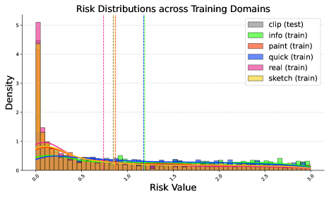
In this paper, we propose to utilise scalar risk distributions as a means to characterise domains, leading to successfully exploring and enforcing domain invariance. Our research reveals that risk distributions can be a reliable indicator of domain variation as it effectively highlights differences between training domains. In Figure 1, we present a visual evidence through histograms, contrasting the risk distributions between the “Art” and “Photo” domains on the validation set of PACS dataset [30], derived from training with Empirical Risk Minimisation (ERM) [57]. The “Photo” domain generally exhibits a larger distribution of scalar risks than that of “Art”. This suggests an inherent complexity in learning “Photo” samples, or possibly due to a more limited training dataset compared to “Art”. During the testing phase, similar divergences between risk distributions may emerge, potentially intensifying in magnitude. Hence, we propose a compelling proposition: by minimising the divergences between risk distributions across training domains, we can achieve robust invariance for DG. The underlying rationale for this concept is that a model, when learning domain-invariant and stable features, tends to produce consistent risk distributions across domains.
Building upon this idea, we propose a novel matching approach for DG, namely Risk Distribution Matching (RDM). RDM’s objective is to minimise the variance of risk distributions across all training domains. Inspired by [38], we redefine the distributional variance metric to focus specifically on risk distributions and propose to compute it via the maximum mean discrepancy (MMD) distance [19]. However, when the number of training domains increases, directly optimising the variance induces a linear growth in MMD computations, reducing efficiency. Instead, we propose an approximation that requires only one MMD computation via aligning just two distributions: that of the worst-case (or worst-performing) domain and the aggregated distribution from all domains. Empirically, this approach outperforms optimising distributional variance while significantly reducing computational complexity. Unlike prevailing matching algorithms, RDM can address the high-dimensional challenges and further improve efficacy by exclusively focusing on scalar risk distributions. Notably, our empirical studies show that RDM even exhibits enhanced generalisation while being more convenient to optimise. We summarise our contributions below:
-
•
We propose RDM, a novel and efficient matching method for DG, based on our two hypotheses: i) risk distribution disparities offer insightful cues into domain variation; ii) reducing these divergences fosters a generalisable and invariant feature-learning predictor.
-
•
We re-conceptualise the distributional variance metric to exclusively focus on risk distributions, with an objective to minimise it. We further provide an approximate version that aligns only the risk distribution of the worst-case domain with the aggregate from all domains, improving both performance and efficiency.
-
•
Through extensive experiments on standard benchmark datasets, we empirically show that RDM consistently outperforms state-of-the-art DG methods, showcasing its remarkable generalisation capability.
2 Related Work
Domain Generalisation (DG)
DG aims to develop models that can generalise well on unseen target domains by leveraging knowledge from multiple source domains. Typical DG methods include domain alignment [38, 7, 32], meta learning [29, 4], data augmentation [63, 61], disentangled representation learning [55, 44], robust optimisation [48, 8] and causality-based methods [25, 13, 41]. Our proposed method RDM is related to domain alignment, striving for domain invariance to enhance OOD generalisation. Existing research focuses on characterising domains through sample representations and aligning their distributions across domains to achieve domain-invariant features [1, 38]. CORAL [54] matches mean and variance of representation distributions, while MMD-AAE [31] and FedKA [56] consider matching all moments via the maxmimum mean discrepancy (MMD) distance [19]. Other methods promote domain invariance by minimising contrastive loss [10] between representations sharing the same labels [35, 37]. Many studies bypass the representation focus, instead characterising domains via gradients and achieving invariance by reducing inter-domain gradient variance [50, 60, 46].
Despite their potential, aligning these high-dimensional distributions may be affected by data sparsity, diversity, and high computational demands [6, 22]. Unlike these methods, RDM offers enhanced efficacy by focusing on scalar risk distributions, overcoming the high-dimensional challenges. Further, RDM adopts a novel strategy by efficiently aligning only two distributions: that of the worst-case domain with the aggregate from all domains. From our experiments, RDM generally exhibits better generalisation performance while being more convenient to optimise compared to competing matching techniques. To the best of our knowledge, the incarnation of risk distributions for domain matching in RDM is novel and sensible.
Distribution matching
Distribution matching has been an important topic with a wide range of applications in machine learning such as DG [31, 54], domain adaptation [59, 9], generative modelling [28, 33]. Early methods, like the MMD distance [19], leverage kernel-based approaches to quantify the distance between distributions, laying the foundation for many subsequent DG techniques [31, 38]. Further advancements have explored optimal transport methods, like the Wasserstein distance [36, 3], which provides a geometrically intuitive means to compare distributions. Other metrics, such as the Kullback-Leibler [26] or Jensen-Shannon [16, 14] divergences, can serve to measure the divergence between distributions and may require additional parameters for estimating the density ratio between the two distributions [53]. In this paper, we utilise the MMD distance to align risk distributions. Its inherent advantages include an analytical measure of the divergence between distributions without relying on distribution densities, and its non-parametric nature [19]. Alternative DG methods augment data by utilising distribution matching and style transfer to generate semantic-preserving samples [62, 63]. Our method differs as we emphasise domain invariance via aligning risk distributions, rather than augmenting representation distributions.
Invariance and Causality in DG
Causal methods in DG assume that the causal mechanism of the target given causal input features is invariant while non-causal features may change across domains [2, 45, 25]. Based on this assumption, methods establish domain invariance to recover the causal mechanism, thereby improving generalisation. ICP [45] has shown that the causal predictor has an invariant distribution of residuals in regression models, however, is not suitable for deep learning. EQRM [13] and REx [25] leverage the invariance in the average risks over samples across domains. In contrast to above methods, we consider matching entire risk distributions over samples across domains, which, as our experiments demonstrate, is more powerful and enhances generalisation capability.
3 Preliminaries
Domain generalisation (DG) involves training a classifier on data composed of multiple training domains (also called environments) so that can perform well on unseen domains at test time. Mathematically, let denote the training set consisting of different domains/environments, and let denote the training data belonging to domain (). Given a loss function , the risk of a particular domain sample is denoted by , and the expected risk of domain is defined as:
| (1) |
A common approach to train is Empirical Risk Minimisation (ERM) [57] which minimises the expected risks across all training domains. Its loss function, denoted by , is computed as follows:
| (2) | ||||
| (3) |
where denotes the set of all domains.
4 Risk Distribution Matching
A model trained via ERM often struggles with generalisation to new test domains. This is because it tends to capture domain-specific features [2, 41], such as domain styles, to achieve low risks in training domains, rather than focusing on domain-invariant or semantic features. To overcome this issue, we present a novel training objective that bolsters generalisation through domain invariance. Our goal requires utilising a unique domain representative that both characterises each domain and provides valuable insights into domain variation. Specifically, we propose to leverage the distribution of risks over all samples within a domain (or shortly risk distribution) as this representative. Unlike other domain representatives, like latent representation or gradient distributions [31, 50], the risk distribution sidesteps high-dimensional challenges like data sparsity and high computational demands [6, 39]. In essence, a model capturing stable, domain-invariant features may consistently yield similar risk distributions across all domains. In pursuit of invariant models, we propose Risk Distribution Matching (RDM), a novel approach for DG that reduces the divergences between training risk distributions via minimising the distributional variance across them.
Let be the probability distribution over the risks of all samples in domain (i.e., ). We refer to as the risk distribution of domain , the representative that effectively captures the core characteristics of the domain. We denote the distributional variance across the risk distributions in the real number space. We achieve our objective by minimising the following loss function:
| (4) |
where is a coefficient balancing between reducing the total training risks with enforcing invariance across domains. is set to 1 unless specified otherwise.
To compute , we require a suitable representation for the implicit risk distribution of domain . Leveraging kernel mean embedding [51], we express as its embedding, , within a reproducing kernel Hilbert space (RKHS) using a feature map below:
| (5) | ||||
| (6) |
where a kernel function is introduced to bypass the explicit specification of . Assuming the condition holds, the mean map remains an element of [19, 31]. It is noteworthy that for a characteristic kernel , the representation within is unique [38, 19]. Consequently, two distinct risk distributions and for any domains respectively have different kernel mean embeddings in . In this work, we use the RBF kernel, a well-known characteristic kernel defined as , where is the bandwidth parameter.
With the unique representation of established, our objective becomes computing the distributional variance between risk distributions within , represented by . Inspired by [38], we redefine the variance metric to focus specifically on risk distributions across multiple domains below:
| (7) |
where denotes the probability distribution over the risks of all samples in the entire training set, or equivalently, the set of all domains. Meanwhile, and represent the mean embedings of and , respectively, and are computed as in Eq. 5. Incorporating into our loss function from Eq. 4, we get:
| (8) |
Minimising in Eq. 8 facilitates our objective of equalising risk distributions across all domains, as proven by the theorem below.
Theorem 1.
[38] Given the distributional variance is calculated with a characteristic kernel , if and only if .
Proof.
Please refer to our appendix for the proof. ∎
In the next part, we present how to compute the distributional variance using the Maximum Mean Discrepancy (MMD) distance [19], relying only on risk samples. Then, we propose an efficient approximation of optimising the distributional variance, yielding improved empirical performance.
4.1 Maximum Mean Discrepancy
For domain , the squared norm, , defined in Eq. 7, is identified as the squared MMD distance [18] between distributions and . It is expressed as follows:
| (9) | ||||
| (10) | ||||
| (11) | ||||
where denote the inner product operation in Through the kernel trick, we can compute these inner products via the kernel function without an explicit form of below:
| (12) | ||||
We reformulate our loss function in Eq. 8 to incorporate MMD as follows:
| (13) | ||||
| (14) |
The loss function involves minimising for every domain . Ideally, the distributional variance reaches its lowest value at if , equivalent to [19, 18], across domains. The objective also entails aligning each individual risk distribution, , with the aggregated distribution spanning all domains, . With the characteristic RBF kernel, it can be viewed as matching an infinite number of moments across all risk distributions.
We emphasise our choice of MMD owing to its benefits for effective risk distribution matching: i) MMD is an important member of the Integral Probability Metric family [40] that offers an analytical solution facilitated through RKHS, and ii) MMD enjoys the property of quantifying the dissimilarity between two implicit distributions via their finite samples in a non-parametric manner.
4.2 Further improvement of RDM
We find that effective alignment of risk distributions across domains can be achieved by matching the risk distribution of the worst-case domain, denoted as , with the combined risk distribution of all domains, offering an approximation to the optimisation of risk distributional variance seen in Eq. 13. This approximate version significantly reduces the MMD distances computation in from to , and further improves generalisation, as we demonstrate with empirical evidence in Section 5.
Denote by the worst-case domain, i.e., the domain that has the largest expected risk in . The approximate RDM’s loss,, is computed as follows:
| (15) | ||||
| (16) |
In our experiments, we observed only a small gap between and , while optimising proving to be more computationally efficient. The key insight emerges from , the first moment (or mean) of . Often, the average risk can serve as a measure of domain uniqueness or divergence [25, 46]. Specifically, a domain with notably distinct mean risk is more likely to diverge greatly from other risk distributions. Under such circumstances, will be an upper-bound of , as shown by: . By optimising , we can also potentially decrease , thus aligning risk distributions across domains effectively. More, drives the model to prioritise the worst-case domain’s optimisation. This approach enhances the model’s robustness to extreme training scenarios, which further improves generalisation as proven in [48, 25]. These insights shed light on the superior performance of optimising over . Therefore, we opted to use , simplifying our model’s training and further bolstering its OOD performance.
5 Experiments
We evaluate and analyse RDM using a synthetic ColoredMNIST dataset [2] and multiple benchmarks from the DomainBed suite [20]. Each of our claims is backed by empirical evidence in this section. Our source code to reproduce results is available at: https://github.com/nktoan/risk-distribution-matching
5.1 Synthetic Dataset: ColoredMNIST
We evaluate all baselines on a synthetic binary classification task, namely ColoredMNIST [2]. This dataset involves categorising digits (0-9) into two labels: “zero” for 0 to 4 range and “one” for 5 to 9 range, with each digit colored either red or green. The dataset is designed to assess the generalisation and robustness of baseline models against the influence of spurious color features. The dataset contains two training domains, where the chance of red digits being classified as “zero” is % and %, respectively, while this probability decreases to only % during testing. The goal is to train a predictor invariant to “digit color” features, capturing only “digit shape” features.
Following [13], we employ a two-hidden-layer MLP with 390 hidden units for all baselines. Optimised through the Adam optimiser [23] at a learning rate of , with a dropout rate of , we train each algorithm for iterations with a batch size of 25,000. We repeat the experiment ten times over different values of the penalty weight . We find our matching penalty quite small, yielding optimal RDM’s performance within the range of . We provide more details about experimental settings in the supplementary material.
| Algorithm | Initialisation | |
|---|---|---|
| Rand. | ERM | |
| ERM | 27.91.5 | 27.91.5 |
| GroupDRO | 27.30.9 | 29.01.1 |
| IGA | 50.71.4 | 57.73.3 |
| IRM | 52.52.4 | 69.70.9 |
| VREx | 55.24.0 | 71.60.5 |
| EQRM | 53.41.7 | 71.40.4 |
| CORAL | 55.32.8 | 65.61.1 |
| MMD | 54.63.2 | 66.41.7 |
| RDM (ours) | 56.31.5 | 72.41.0 |
| Oracle | 72.10.7 | |
| Optimum | 75.0 | |


We compare RDM with ERM and three different types of algorithms: robust optimisation (GroupDRO [48], IGA [24]), causal methods learning invariance (IRM [2], VREx [25], EQRM [13]) and representation distribution matching (MMD [31], CORAL [54]). All algorithms are run using two distinct network configurations: (i) initialising the network randomly via Xavier method [17]; (ii) pre-training the network with ERM for iterations prior to performing the algorithms. Table 1 shows that our proposed method RDM surpasses all algorithms, irrespective of the network configuration. RDM exhibits improvements of % and % over CORAL, both without and with pre-trained ERM, respectively, underlining the effectiveness of aligning risk distributions instead of high-dimensional representations. VREx and EQRM, which pursue invariant predictors by equalising average training risks across domains, demonstrate suboptimal performance compared to our approach. This improvement arises from our consideration of the entire risk distributions and the matching of all moments across them, which inherently foster stronger invariance for DG. Notably, all methods experience enhanced performance with ERM initialisation. RDM even excels beyond oracle performance (ERM trained on grayscale digits with 50% red and 50% green) and converges towards optimality.
Figure 2 demonstrates histograms with their KDE curves [42] depicting the risk distributions of ERM and RDM across four domains. The figure confirms our hypothesis that the disparities among risk distributions could serve as a valuable signal of domain variation. ERM’s histogram shows a clear difference between environments with % and % chance of red digits labelled “zero” and those with only % or %. More, ERM tends to overfit to training domains, which negatively impacts its generalisation to test domains. Remarkably, RDM effectively minimises the divergences between risk distributions across all domains, including test domains with lower risks. This also aligns with our motivation: an invariant or stable feature-learning predictor, by displaying similar risk distributions across domains, inherently boosts generalisation.
5.2 DomainBed
| Algorithm | VLCS | PACS | OfficeHome | TerraIncognita | DomainNet | Avg |
|---|---|---|---|---|---|---|
| ERM | 77.50.4 | 85.50.2 | 66.50.3 | 46.11.8 | 40.90.1 | 63.3 |
| Mixup | 77.40.6 | 84.60.6 | 68.10.3 | 47.90.8 | 39.20.1 | 63.4 |
| MLDG | 77.20.4 | 84.91.0 | 66.80.6 | 47.70.9 | 41.20.1 | 63.6 |
| GroupDRO | 76.70.6 | 84.40.8 | 66.00.7 | 43.21.1 | 33.30.2 | 60.9 |
| IRM | 78.50.5 | 83.50.8 | 64.32.2 | 47.60.8 | 33.92.8 | 61.6 |
| VREx | 78.30.2 | 84.90.6 | 66.40.6 | 46.40.6 | 33.62.9 | 61.9 |
| EQRM | 77.80.6 | 86.50.2 | 67.50.1 | 47.80.6 | 41.00.3 | 64.1 |
| Fish | 77.80.3 | 85.50.3 | 68.60.4 | 45.11.3 | 42.70.2 | 64.0 |
| Fishr | 77.80.1 | 85.50.4 | 67.80.1 | 47.41.6 | 41.70.0 | 64.0 |
| CORAL | 78.80.6 | 86.20.3 | 68.70.3 | 47.61.0 | 41.50.1 | 64.6 |
| MMD | 77.50.9 | 84.60.5 | 66.30.1 | 42.21.6 | 23.49.5 | 63.3 |
| RDM (ours) | 78.40.4 | 87.20.7 | 67.30.4 | 47.51.0 | 43.40.3 | 64.8 |
Dataset and Protocol
Following previous works [20, 13], we extensively evaluate all methods on five well-known DG benchmarks: VLCS [15], PACS [30], OfficeHome [58], TerraIncognita [5], and DomainNet [43]. For a fair comparison, we reuse the training and evaluation protocol in DomainBed [20], including the dataset splits, training iterations, and model selection criteria. Our evaluation employs the leave-one-domain-out approach: each model is trained on all domains except one and then tested on the excluded domain. The final model is chosen based on its combined accuracy across all training-domain validation sets.
Implementation Details
We use ResNet-50 [21] pre-trained on ImageNet [47] as the default backbone. The model is optimised via the Adam optimiser for iterations on every dataset. We follow [13, 25] to pre-train baselines with ERM for certain iterations before performing the algorithms. Importantly, we find that achieving accurate risk distribution matching using distribution samples requires larger batch sizes - details of which are examined in our ablation studies. For most datasets, the optimal batch size lies between . However, for huge datasets like TerraIncognita and DomainNet, it is between . Although computational resources limit us from testing larger batch sizes, these ranges consistently achieve strong performance on benchmarks. The matching coefficient in our method is set in . Additional hyper-parameters like learning rate, dropout rate, or weight decay, adhere to the preset ranges as detailed in [13]. We provide more implementation details in the supplementary material. We repeat our experiments ten times with varied seed values and hyper-parameters and report the average results.
Experimental Results
In Table 2, we show the average out-of-domain (OOD) accuracies of state-of-the-art DG methods on five benchmarks. Due to space constraints, domain-specific accuracies are detailed in the supplementary material. We compare RDM with ERM and various types of algorithms: distributional robustness (GroupDRO), causal methods learning invariance (IRM, VREx, EQRM), gradient matching (Fish [50], Fishr [46]), representation distribution matching (MMD, CORAL) and other variants (Mixup [61], MLDG [29]). To ensure fairness in our evaluations, we have used the same training data volume across all baselines, although further employing augmentations can enhance models’ performance.
On average, RDM surpasses other baselines across all benchmarks, notably achieving a % average improvement over ERM. The significant improvement of RDM on DomainNet, a large-scale dataset with 586,575 images across 6 domains, is worth mentioning. This suggests that characterising domains with risk distributions to achieve invariance effectively enhances OOD performance. Compared to distributional robustness methods, RDM notably outperforms GroupDRO with improvement of % on PACS and a substantial % on DomainNet. RDM consistently improves over causality-based methods that rely on the average risk for domain invariance. This superiority attributes to our novel adoption of risk distributions, achieving enhanced invariance for DG. Our remarkable improvement over MMD suggests that aligning risk distributions via the MMD distance is more effective, easier to optimise than aligning representation distributions. While RDM typically outperforms CORAL and Fish in OOD scenarios, it only remains competitive or sometimes underperforms on certain datasets like OfficeHome. This decrease in performance may stem from the dataset’s inherent tendency to overfit within our risk distribution alignment objective. OfficeHome has only average about 240 samples per class, significantly fewer than other datasets with at least 1,400. This reduced sample size may not provide sufficiently diverse risk distributions to capture stable class features, resulting in overfitting on the training set. Despite these limitations, our OfficeHome results still outperform several well-known baselines such as MLDG, VREx, or ERM. For a detailed discussion on this challenge, please refer to our supplementary material.
5.3 Analysis


In this section, we provide empirical evidence backing our claims in Section 4. In Figure LABEL:fig:analysis_A-small-gap, we highlight a small gap when aligning the risk distribution of the worst-case domain with that of all domains combined (RDM with ), compared to directly optimising the distributional variance (RDM with ). Notably, consistently represents an upper bound of , which is sensible since the worst-case domain often exhibits the most distinct risk distribution. This suggests that optimising also helps reduce the distributional variance , bringing the risk distributions across domains closer.
| Algorithm | Training (s) | Mem (GiB) | Acc (%) |
|---|---|---|---|
| Fish | 11,502 | 5.26 | 42.7 |
| CORAL | 11,504 | 17.00 | 41.5 |
| RDM with | 9,854 | 16.94 | 43.1 |
| RDM with | 7,749 | 16.23 | 43.4 |
When the number of training domains grows, especially with large-scale datasets like DomainNet, emphasising the risk distribution of the worst-case domain not only proves to be a more efficient approach but also significantly enhances OOD performance. In our exploration of training resources for DomainNet, we study three matching methods: Fish, CORAL and two variants of our RDM method. For a fair evaluation, all experiments were conducted with identical GPU resources, settings, and hyper-parameters, such as batch size or training iterations. Results can be seen in Table 3. Full details on training resources for these methods on other datasets are available in the supplementary material due to space constraints.
Our RDM with the objective proves fastest in training and achieves the notably highest % accuracy on DomainNet. While RDM demands more memory than Fish, due to the storage of MMD distance values, it can be trained in less time - under an hour - and still delivers a % performance boost. This gain over Fish, a leading gradient maching method on DomainNet, is significant. Among two variants of RDM, the one using is both the fastest and most accurate, justifying our claims on the benefits of aligning the risk distribution of the worst-case domain.
More, to further highlight the efficacy of risk distribution alignment for DG, we compare the OOD performance learning curves of RDM with competing baselines using representation (CORAL) and gradient (Fish) alignments, as depicted in Figure LABEL:fig:analysis_Learning-curves. Impressively, RDM consistently outperforms, demonstrating enhanced generalisation throughout the training process.
5.4 Ablation studies
We explore the impact of the matching coefficient and training batch size on risk distribution matching, using primarily the PACS dataset for brevity. While other datasets exhibit similar trends, their detailed results are provided in the supplementary material.
Matching coefficient
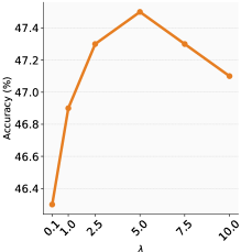
Figure LABEL:fig:ablation_study_lambda illustrates the performance of RDM on the PACS dataset for varying values of the matching coefficient , spanning . Notably, as increases, RDM’s accuracy consistently improves, justifying the significance of our risk distribution matching module in fostering generalisation. In particular, when , RDM demonstrates a notable % average accuracy boost across all domains, in contrast to when using only . Across most datasets, a value within appears sufficient to produce good results.
Batch size
We study the impact of batch size on RDM’s performance. Our assumption is that achieving accurate risk distribution matching through data samples would require larger batch sizes. Figure LABEL:fig:ablation_study_batchsize validates this, revealing enhanced generalisation results on PACS with increased batch sizes. For PACS, sizes between yield promising, potentially optimal outcomes, despite computational limitations restrict our exploration of larger sizes.


6 Conclusion
We have demonstrated that RDM, a novel matching method for domain generalisation (DG), provides enhanced generalisation capability by aligning risk distributions across domains. RDM efficiently overcomes high-dimensional challenges of conventional DG matching methods. RDM is built on our observation that risk distributions can effectively represent the differences between training domains. By minimising these divergences, we can achieve an invariant and generalisable predictor. We further improve RDM by matching only the risk distribution of the worst-case domain with the aggregate from all domains, bypassing the need to directly compute the distributional variance. This approximate version not only offers computational efficiency but also delivers improved out-of-domain results. Our extensive experiments on several benchmarks reveal that RDM surpasses leading DG techniques. We hope our work can inspire further investigations into the benefits of risk distributions for DG.
References
- [1] Isabela Albuquerque, João Monteiro, Mohammad Darvishi, Tiago H Falk, and Ioannis Mitliagkas. Generalizing to unseen domains via distribution matching. arXiv preprint arXiv:1911.00804, 2019.
- [2] Martin Arjovsky, Léon Bottou, Ishaan Gulrajani, and David Lopez-Paz. Invariant risk minimization. arXiv preprint arXiv:1907.02893, 2019.
- [3] Martin Arjovsky, Soumith Chintala, and Léon Bottou. Wasserstein generative adversarial networks. In ICML, pages 214–223, 2017.
- [4] Yogesh Balaji, Swami Sankaranarayanan, and Rama Chellappa. Metareg: Towards domain generalization using meta-regularization. NIPS, 31, 2018.
- [5] Sara Beery, Grant Van Horn, and Pietro Perona. Recognition in terra incognita. In ECCV, pages 456–473, 2018.
- [6] Richard Bellman. Dynamic programming. Science, 153(3731):34–37, 1966.
- [7] Shai Ben-David, John Blitzer, Koby Crammer, Alex Kulesza, Fernando Pereira, and Jennifer Wortman Vaughan. A theory of learning from different domains. Machine learning, 79:151–175, 2010.
- [8] Peter Bühlmann. Invariance, causality and robustness. 2020.
- [9] Chaoqi Chen, Weiping Xie, Wenbing Huang, Yu Rong, Xinghao Ding, Yue Huang, Tingyang Xu, and Junzhou Huang. Progressive feature alignment for unsupervised domain adaptation. In CVPR, pages 627–636, 2019.
- [10] Ting Chen, Simon Kornblith, Mohammad Norouzi, and Geoffrey Hinton. A simple framework for contrastive learning of visual representations. In ICML, pages 1597–1607, 2020.
- [11] Mathieu Chevalley, Charlotte Bunne, Andreas Krause, and Stefan Bauer. Invariant causal mechanisms through distribution matching. arXiv preprint arXiv:2206.11646, 2022.
- [12] Andrea Dittadi, Frederik Träuble, Francesco Locatello, Manuel Wüthrich, Vaibhav Agrawal, Ole Winther, Stefan Bauer, and Bernhard Schölkopf. On the transfer of disentangled representations in realistic settings. ICLR, 2021.
- [13] Cian Eastwood, Alexander Robey, Shashank Singh, Julius Von Kügelgen, Hamed Hassani, George J Pappas, and Bernhard Schölkopf. Probable domain generalization via quantile risk minimization. NeurIPS, 35:17340–17358, 2022.
- [14] Dominik Maria Endres and Johannes E Schindelin. A new metric for probability distributions. IEEE Transactions on Information theory, pages 1858–1860, 2003.
- [15] Chen Fang, Ye Xu, and Daniel N Rockmore. Unbiased metric learning: On the utilization of multiple datasets and web images for softening bias. In ICCV, pages 1657–1664, 2013.
- [16] Bent Fuglede and Flemming Topsoe. Jensen-shannon divergence and hilbert space embedding. In ISIT, page 31. IEEE, 2004.
- [17] Xavier Glorot and Yoshua Bengio. Understanding the difficulty of training deep feedforward neural networks. In AISTATS, pages 249–256, 2010.
- [18] Arthur Gretton, Karsten Borgwardt, Malte Rasch, Bernhard Schölkopf, and Alex Smola. A kernel method for the two-sample-problem. NIPS, 19, 2006.
- [19] Arthur Gretton, Karsten M Borgwardt, Malte J Rasch, Bernhard Schölkopf, and Alexander Smola. A kernel two-sample test. JMLR, pages 723–773, 2012.
- [20] Ishaan Gulrajani and David Lopez-Paz. In search of lost domain generalization. In ICLR, 2021.
- [21] Kaiming He, Xiangyu Zhang, Shaoqing Ren, and Jian Sun. Deep residual learning for image recognition. In CVPR, pages 770–778, 2016.
- [22] Piotr Indyk and Rajeev Motwani. Approximate nearest neighbors: towards removing the curse of dimensionality. In Proc. Annu. ACM Symp. Theory Comput., pages 604–613, 1998.
- [23] Diederik P Kingma and Jimmy Ba. Adam: A method for stochastic optimization. ICLR, 2015.
- [24] Masanori Koyama and Shoichiro Yamaguchi. Out-of-distribution generalization with maximal invariant predictor. 2020.
- [25] David Krueger, Ethan Caballero, Joern-Henrik Jacobsen, Amy Zhang, Jonathan Binas, Dinghuai Zhang, Remi Le Priol, and Aaron Courville. Out-of-distribution generalization via risk extrapolation (rex). In ICML, pages 5815–5826, 2021.
- [26] Solomon Kullback and Richard A Leibler. On information and sufficiency. The annals of mathematical statistics, 22(1):79–86, 1951.
- [27] Yann LeCun, Yoshua Bengio, and Geoffrey Hinton. Deep learning. Nature, 521(7553):436–444, 2015.
- [28] Chun-Liang Li, Wei-Cheng Chang, Yu Cheng, Yiming Yang, and Barnabás Póczos. Mmd-gan: Towards deeper understanding of moment matching network. NIPS, 30, 2017.
- [29] Da Li, Yongxin Yang, Yi-Zhe Song, and Timothy Hospedales. Learning to generalize: Meta-learning for domain generalization. In AAAI, volume 32, 2018.
- [30] Da Li, Yongxin Yang, Yi-Zhe Song, and Timothy M Hospedales. Deeper, broader and artier domain generalization. In ICCV, pages 5542–5550, 2017.
- [31] Haoliang Li, Sinno Jialin Pan, Shiqi Wang, and Alex C Kot. Domain generalization with adversarial feature learning. In CVPR, pages 5400–5409, 2018.
- [32] Ya Li, Mingming Gong, Xinmei Tian, Tongliang Liu, and Dacheng Tao. Domain generalization via conditional invariant representations. In AAAI, volume 32, 2018.
- [33] Yujia Li, Kevin Swersky, and Rich Zemel. Generative moment matching networks. In ICML, pages 1718–1727, 2015.
- [34] Chaochao Lu, Yuhuai Wu, José Miguel Hernández-Lobato, and Bernhard Schölkopf. Invariant causal representation learning for out-of-distribution generalization. In ICLR, 2021.
- [35] Divyat Mahajan, Shruti Tople, and Amit Sharma. Domain generalization using causal matching. In ICML, pages 7313–7324, 2021.
- [36] Facundo Mémoli. Gromov–wasserstein distances and the metric approach to object matching. Foundations of computational mathematics, 11:417–487, 2011.
- [37] Saeid Motiian, Marco Piccirilli, Donald A Adjeroh, and Gianfranco Doretto. Unified deep supervised domain adaptation and generalization. In ICCV, pages 5715–5725, 2017.
- [38] Krikamol Muandet, David Balduzzi, and Bernhard Schölkopf. Domain generalization via invariant feature representation. In ICML, pages 10–18, 2013.
- [39] Marius Muja and David G Lowe. Scalable nearest neighbor algorithms for high dimensional data. TPAMI, 36(11):2227–2240, 2014.
- [40] Alfred Müller. Integral probability metrics and their generating classes of functions. Advances in applied probability, 29(2):429–443, 1997.
- [41] Toan Nguyen, Kien Do, Duc Thanh Nguyen, Bao Duong, and Thin Nguyen. Causal inference via style transfer for out-of-distribution generalisation. In KDD, pages 1746–1757, 2023.
- [42] Emanuel Parzen. On estimation of a probability density function and mode. The annals of mathematical statistics, 33(3):1065–1076, 1962.
- [43] Xingchao Peng, Qinxun Bai, Xide Xia, Zijun Huang, Kate Saenko, and Bo Wang. Moment matching for multi-source domain adaptation. In ICCV, pages 1406–1415, 2019.
- [44] Xingchao Peng, Zijun Huang, Ximeng Sun, and Kate Saenko. Domain agnostic learning with disentangled representations. In ICML, pages 5102–5112, 2019.
- [45] Jonas Peters, Peter Bühlmann, and Nicolai Meinshausen. Causal inference by using invariant prediction: identification and confidence intervals. Journal of the Royal Statistical Society Series B: Statistical Methodology, 78(5):947–1012, 2016.
- [46] Alexandre Rame, Corentin Dancette, and Matthieu Cord. Fishr: Invariant gradient variances for out-of-distribution generalization. In ICML, pages 18347–18377, 2022.
- [47] Olga Russakovsky, Jia Deng, Hao Su, Jonathan Krause, Sanjeev Satheesh, Sean Ma, Zhiheng Huang, Andrej Karpathy, Aditya Khosla, Michael Bernstein, Alexander C. Berg, and Li Fei-Fei. ImageNet Large Scale Visual Recognition Challenge. IJCV, 115(3):211–252, 2015.
- [48] Shiori Sagawa, Pang Wei Koh, Tatsunori B Hashimoto, and Percy Liang. Distributionally robust neural networks for group shifts: On the importance of regularization for worst-case generalization. In ICLR, 2020.
- [49] Vaishaal Shankar, Achal Dave, Rebecca Roelofs, Deva Ramanan, Benjamin Recht, and Ludwig Schmidt. Do image classifiers generalize across time? In ICCV, pages 9661–9669, 2021.
- [50] Yuge Shi, Jeffrey Seely, Philip Torr, Siddharth N, Awni Hannun, Nicolas Usunier, and Gabriel Synnaeve. Gradient matching for domain generalization. In ICLR, 2022.
- [51] Alex Smola, Arthur Gretton, Le Song, and Bernhard Schölkopf. A hilbert space embedding for distributions. In International conference on algorithmic learning theory, pages 13–31, 2007.
- [52] Bharath K Sriperumbudur, Arthur Gretton, Kenji Fukumizu, Bernhard Schölkopf, and Gert RG Lanckriet. Hilbert space embeddings and metrics on probability measures. JMLR, 11:1517–1561, 2010.
- [53] Masashi Sugiyama, Taiji Suzuki, and Takafumi Kanamori. Density ratio estimation in machine learning. Cambridge University Press, 2012.
- [54] Baochen Sun and Kate Saenko. Deep coral: Correlation alignment for deep domain adaptation. In ECCV Workshops, pages 443–450. Springer, 2016.
- [55] Xinwei Sun, Botong Wu, Xiangyu Zheng, Chang Liu, Wei Chen, Tao Qin, and Tie-Yan Liu. Recovering latent causal factor for generalization to distributional shifts. NeurIPS, 34:16846–16859, 2021.
- [56] Yuwei Sun, Ng Chong, and Hideya Ochiai. Feature distribution matching for federated domain generalization. In ACML, pages 942–957, 2023.
- [57] Vladimir N Vapnik. An overview of statistical learning theory. IEEE transactions on neural networks, 10(5):988–999, 1999.
- [58] Hemanth Venkateswara, Jose Eusebio, Shayok Chakraborty, and Sethuraman Panchanathan. Deep hashing network for unsupervised domain adaptation. In CVPR, pages 5018–5027, 2017.
- [59] Jindong Wang, Wenjie Feng, Yiqiang Chen, Han Yu, Meiyu Huang, and Philip S Yu. Visual domain adaptation with manifold embedded distribution alignment. In ACMMM, pages 402–410, 2018.
- [60] Pengfei Wang, Zhaoxiang Zhang, Zhen Lei, and Lei Zhang. Sharpness-aware gradient matching for domain generalization. In CVPR, pages 3769–3778, 2023.
- [61] Hongyi Zhang, Moustapha Cisse, Yann N Dauphin, and David Lopez-Paz. mixup: Beyond empirical risk minimization. ICLR, 2018.
- [62] Yabin Zhang, Minghan Li, Ruihuang Li, Kui Jia, and Lei Zhang. Exact feature distribution matching for arbitrary style transfer and domain generalization. In CVPR, pages 8035–8045, 2022.
- [63] Kaiyang Zhou, Yongxin Yang, Yu Qiao, and Tao Xiang. Domain generalization with mixstyle. In ICLR, 2021.
7 Supplementary Material
In this supplementary material, we first provide a detailed proof for our theorem on distributional variance, as outlined in Section 8. Next, in Section 9, we detail more about our experimental settings, covering both the ColoredMNIST synthetic dataset [2] and the extensive benchmarks from the DomainBed suite [20] in the main text. Additional ablation studies and discussions on our proposed method are given in Section 10. Finally, Section 11 provides domain-specific out-of-domain accuracies for each dataset within the DomainBed suite.
8 Theoretical Results
We provide the proof for the theorem on distributional variance discussed in the main paper. We revisit the concept of kernel mean embedding [51] to express the risk distribution of domain . Particularly, we represent through its embedding, , in a reproducing kernel Hilbert space (RKHS) denoted as . This is achieved by using a feature map below:
| (17) | ||||
| (18) |
where a kernel function is introduced to bypass the explicit specification of .
Theorem.
[38] Denote the probability distribution over the risks of all samples in the entire training set, or equivalently, the set of all domains. Given the distributional variance is calculated with a characteristic kernel , if and only if .
Proof.
In our methodology, we employ the RBF kernel, which is characteristic in nature. As a result, the term acts as a metric within the Hilbert space [38]. Importantly, this metric reaches zero if and only if [52]. Let’s consider the distributional variance, , which is defined below:
| (19) |
This variance becomes zero if and only if for each . This logically implies that for all , leading to .
Conversely, we assume that . Given this condition, for any , it follows that:
| (20) |
which implies
| (21) |
Consequently, by the given definition of distributional variance, we have: . This completes the proof. ∎
9 More implementation details
For our experiments, we leveraged the PyTorch DomainBed toolbox [20, 13] and utilised an Ubuntu 20.4 server outfitted with a 36-core CPU, 767GB RAM, and NVIDIA V100 32GB GPUs. The software stack included Python 3.11.2, PyTorch 1.7.1, Torchvision 0.8.2, and Cuda 12.0. Additional implementation details, beyond the hyper-parameters discussed in the main text, are elaborated below.
9.1 ColoredMNIST
In alignment with [13], we performed experiments on the ColoredMNIST dataset, the results of which are detailed in Table 1 in the main paper. We partitioned the original MNIST training dataset into distinct training and validation sets of 25,000 and 5,000 samples for each of two training domains, respectively. The original MNIST test set was adapted to function as our test set. Particularly, we synthesised this test set to introduce a distribution shift: red digits have only a % probability of being classified as “zero”, compared to 80% and 90% in the training sets for different domains. Besides the hyper-parameters highlighted in the main paper, we also leveraged a cosine annealing scheduler to further optimise the training process like other baselines.
For our RDM method, we constrained the alignment to focus only on the first two empirical moments (mean and variance) of and . We experimented with five different penalty weight values for in the range of , running each experiment ten times and varying . The reported results are the average accuracies and their standard deviations over these 10 runs, all measured on a test-domain test set. We adhered to test-domain validation for model selection across all methods, as recommended by [20]. We reference results for other methods from [13].
9.2 DomainBed
9.2.1 Description of benchmarks
| Parameter | Dataset | Default value | Random distribution |
|---|---|---|---|
| steps | All | 5,000 | 5,000 |
| learning rate | All | ||
| dropout | All | 0 | RandomChoice |
| weight decay | All | 0 | |
| batch size | PACS / VLCS / OfficeHome | 88 | Uniform() |
| TerraIncognita / DomainNet | 40 | Uniform() | |
| matching coefficient | All except DomainNet | 5.0 | Uniform() |
| DomainNet | 0.5 | Uniform() | |
| pre-trained iterations | All except DomainNet | 1500 | Uniform() |
| DomainNet | 2400 | Uniform() | |
| learning rate after pre-training | All | Uniform() | |
| variance regularisation coefficient | PACS / VLCS | 0.004 | Uniform() |
| OfficeHome / TerraIncognita / | |||
| DomainNet | 0 | 0 |
For our evaluations, we leveraged five large-scale benchmark datasets from the DomainBed suite [20], comprising:
-
•
VLCS [15]: The dataset encompasses four photographic domains: Caltech101, LabelMe, SUN09, VOC2007. It contains 10,729 examples, each with dimensions , and spans five distinct classes.
-
•
PACS [30]: The dataset includes 9,991 images from four different domains: Photo (P), Art-painting (A), Cartoon (C), and Sketch (S). These domains each have their own unique style, making this dataset particularly challenging for out-of-distribution (OOD) generalisation. Each domain has seven classes.
-
•
OfficeHome [58]: The dataset features 15,500 images of objects commonly found in office and home settings, categorised into 65 classes. These images are sourced from four distinct domains: Art (A), Clipart (C), Product (P), and Real-world (R).
-
•
TerraIncognita [5]: The dataset includes 24,788 camera-trap photographs of wild animals captured at locations . Each image has dimensions and falls into one of 10 distinct classes.
-
•
DomainNet [43]: The largest dataset in DomainBed, DomainNet, contains 586,575 examples in dimensions , spread across six domains and encompassing 345 classes.
9.2.2 Our implementation details
| Algorithm | Training (s) | Mem (GiB) | Acc (%) |
|---|---|---|---|
| Fish | 7,566 | 7.97 | 85.5 |
| CORAL | 4,485 | 21.81 | 86.2 |
| RDM with | 4,783 | 21.87 | 86.6 |
| RDM with | 4,214 | 21.71 | 87.2 |
| Algorithm | Training (s) | Mem (GiB) | Acc (%) |
|---|---|---|---|
| Fish | 13,493 | 7.97 | 77.8 |
| CORAL | 6,329 | 21.81 | 78.8 |
| RDM with | 9,441 | 21.87 | 77.8 |
| RDM with | 6,151 | 21.71 | 78.4 |
| Algorithm | Training (s) | Mem (GiB) | Acc (%) |
|---|---|---|---|
| Fish | 9,035 | 7.97 | 68.6 |
| CORAL | 4,762 | 21.81 | 68.7 |
| RDM with | 5,467 | 21.87 | 67.0 |
| RDM with | 4,588 | 21.71 | 67.3 |
| Algorithm | Training (s) | Mem (GiB) | Acc (%) |
|---|---|---|---|
| Fish | 6,019 | 4.08 | 45.1 |
| CORAL | 2,973 | 10.21 | 47.6 |
| RDM with | 4,040 | 10.17 | 47.1 |
| RDM with | 2,697 | 10.11 | 47.5 |
To ensure rigorous evaluation and a fair comparison with existing baselines [13, 46], we conducted experiments on five datasets from the DomainBed suite, the results of which are elaborated in Table 2 of the main text. In alignment with standard practices, we optimised hyper-parameters for each domain through a randomised search across 20 trials on the validation set, utilising a joint distribution as specified in Table 9.2.1. The dataset from each domain was partitioned into an 80% split for training and testing, and a 20% split for hyper-parameter validation. A comprehensive discussion on the hyper-parameters used in our experiments is provided below. For each domain, we performed our experiments ten times, employing varied seed values and hyper-parameters within the specified range, and reported the averaged results with their standard deviations. We reference results for other methods from [13, 46]. We kindly refer readers to our given source code for more detail.
In our methodology, we employed the MMD distance for aligning risk distributions and , as described in Section 4. Utilising the RBF kernel, we compute the average MMD distance across an expansive bandwidth spectrum , bypassing the need for tuning this parameter.
Inspired by recent insights [13], we incorporated an initial pre-training-with-ERM phase to further improve the OOD performance. DomainNet, given its scale, requires longer ERM pre-training; specific parameters for all datasets are provided in Table 9.2.1. Our initial learning rate lies within , which adapts to post-ERM pre-training. Incorporating additional variance regularisation on and proves beneficial for the PACS and VLCS datasets. This approach constrains the induced risks to fall within narrower, more optimal value ranges, facilitating more effective risk distribution alignment. Optimal regularisation coefficients for this strategy are detailed in Table 9.2.1.
We maintain minimal dropout and weight decay, reserving our focus for risk distribution alignment. Optimal batch sizes differ: for VLCS and OfficeHome, and for TerraIncognita and DomainNet. Despite computational constraints limiting our ability to test larger batch sizes, the selected ranges yield robust performance across datasets.
Regarding the matching coefficient in our objective, most datasets work well within , but DomainNet prefers a narrower range. This fine-tuning is key, especially for large-scale datasets, to balance risk reduction and cross-domain alignment in the early training stages.
10 More ablation studies and analyses
10.1 Efficacy of DG matching methods
Table 5 compares the efficiency and effectiveness of various methods: Fish, CORAL, RDM with , and RDM with across several benchmarks - PACS, VLCS, OfficeHome, and TerraIncognita. Notably, the approximate variant, denoted as RDM with , stands out for its exceptional performance. This version emphasises the alignment of risk distribution for the worst-case domain and exhibits both faster training times and improved accuracy over its counterpart that optimises distributional variance, RDM with . For instance, on the VLCS dataset, this variant is trained in under an hour while achieving a % accuracy boost.
When compared to the gradient-matching Fish method, our approach demonstrates similar advantages but requires additional memory to store MMD distance values. The memory constraint is not unique to our method; CORAL also encounters this limitation. However, RDM outperforms CORAL in both training time and memory usage, especially evident on large-scale datasets like DomainNet. This efficiency gain is noteworthy, given that CORAL’s increased computational requirements arise from its handling of high-dimensional representation vectors.
In terms of the accuracy, as confirmed by our main text, RDM outperforms CORAL substantially on both PACS and DomainNet, while maintaining competitiveness on TerraIncognita and VLCS. On OfficeHome, although RDM lags behind CORAL, we provide an in-depth explanation for this behavior both in the main text and in the subsequent section.
10.2 Decreased Performance on OfficeHome
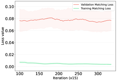
In our evaluation, RDM generally surpasses competing matching methods in OOD settings but faces challenges in specific datasets like OfficeHome. The dataset’s limitations are noteworthy: with an average of only 240 samples per class, OfficeHome has significantly fewer instances per class than other datasets, which usually have at least 1,400. This limited sample size may constrain the model from learning sufficiently class-semantic features or diverse risk distributions, leading to overfitting on the training set. To shed light on this issue, we present a visual analysis in Figure 5. Starting from the 100th iteration, when we perform the task of matching risk distributions, we note that the training matching loss is already minimal, forming a clear divergence with the validation matching loss. While the training loss continues to converge to minimal values, the validation loss remains inconsistent throughout the training phase. This inconsistency showcases that the limited diversity in OfficeHome’s risk distributions may induce the model’s overfitting on training samples, reducing its generalisation capabilities. Despite these constraints, our method still outperforms other well-known baselines, such as MLDG, VREx, and ERM, on OfficeHome.
10.3 Impact of batch size and matching coefficient


In our analysis, we closely examine how batch size and the matching coefficient affect RDM’s performance across four benchmark datasets: VLCS, OfficeHome, TerraIncognita, and DomainNet. Consistent with our main text findings on PACS, Figure 6 shows that using larger batch sizes enhances the model’s generalisation by facilitating accurate risk distribution matching. Similarly, Figure 7 highlights the importance of in improving OOD performance; as increases, OOD performance generally improves.
We find optimal batch size ranges for each dataset: VLCS and OfficeHome perform best with sizes between , while the larger datasets of TerraIncognita and DomainNet benefit from a more limited range of . Even with computational limitations, these batch sizes lead to strong performance. For most datasets, a value between is effective. In the case of DomainNet, a smaller range of works well, balancing the reduction of training risks and the alignment of risk distributions across domains. This is particularly important for large-scale datasets where reducing training risks is crucial for learning predictive features, especially during the initial phases of training.
10.4 Risk distributions


We present visualisations of risk distribution histograms accompanied by their KDE curves for two datasets, PACS and DomainNet, in Figures 8 and 9, respectively. These visualisations compare the risk distributions of ERM and our proposed RDM method on the validation sets. Both figures confirm our hypothesis that variations in training domains lead to distinct risk distributions, making them valuable indicators of domain differences.
On PACS, we observe that ERM tends to capture domain-specific features, resulting in low risks within the training domains. However, ERM’s substantial deviation of the average risk for the test domain from that for the training domains suggests sub-optimal OOD generalisation. In contrast, our RDM approach prioritises stable, domain-invariant features, yielding more consistent risk distributions and enhanced generalisation. This trend holds across both two datasets, as our approach consistently aligns risk distributions across domains better than ERM. This alignment effectively narrows the gap between test and training domains, especially reducing risks for test domains.
These findings underscore the efficacy of our RDM method in mitigating domain variations by aligning risk distributions, ultimately leading to enhanced generalisation.
11 More experimental results
We provide domain-specific out-of-domain accuracies for each dataset within the DomainBed suite in Tables 6, 7, 8, 9, 10. In each table, the accuracy listed in each column represents the out-of-domain performance when that specific domain is excluded from the training set and used solely for testing within the respective dataset. We note that the per-domain results for Fish [50] are not available.
| Algorithm | clip | info | paint | quick | real | sketch | Avg |
|---|---|---|---|---|---|---|---|
| ERM | 58.1 0.3 | 18.8 0.3 | 46.7 0.3 | 12.2 0.4 | 59.6 0.1 | 49.8 0.4 | 40.9 |
| Mixup | 55.7 0.3 | 18.5 0.5 | 44.3 0.5 | 12.5 0.4 | 55.8 0.3 | 48.2 0.5 | 39.2 |
| MLDG | 59.1 0.2 | 19.1 0.3 | 45.8 0.7 | 13.4 0.3 | 59.6 0.2 | 50.2 0.4 | 41.2 |
| GroupDRO | 47.2 0.5 | 17.5 0.4 | 33.8 0.5 | 9.3 0.3 | 51.6 0.4 | 40.1 0.6 | 33.3 |
| IRM | 48.5 2.8 | 15.0 1.5 | 38.3 4.3 | 10.9 0.5 | 48.2 5.2 | 42.3 3.1 | 33.9 |
| VREx | 47.3 3.5 | 16.0 1.5 | 35.8 4.6 | 10.9 0.3 | 49.6 4.9 | 42.0 3.0 | 33.6 |
| EQRM | 56.1 1.3 | 19.6 0.1 | 46.3 1.5 | 12.9 0.3 | 61.1 0.0 | 50.3 0.1 | 41.0 |
| Fish | - | - | - | - | - | - | 42.7 |
| Fishr | 58.2 0.5 | 20.2 0.2 | 47.7 0.3 | 12.7 0.2 | 60.3 0.2 | 50.8 0.1 | 41.7 |
| CORAL | 59.2 0.1 | 19.7 0.2 | 46.6 0.3 | 13.4 0.4 | 59.8 0.2 | 50.1 0.6 | 41.5 |
| MMD | 32.1 13.3 | 11.0 4.6 | 26.8 11.3 | 8.7 2.1 | 32.7 13.8 | 28.9 11.9 | 23.4 |
| RDM (ours) | 62.1 0.2 | 20.7 0.1 | 49.2 0.4 | 14.1 0.4 | 63.0 1.3 | 51.4 0.1 | 43.4 |
| Algorithm | A | C | P | S | Avg |
|---|---|---|---|---|---|
| ERM | 84.7 0.4 | 80.8 0.6 | 97.2 0.3 | 79.3 1.0 | 85.5 |
| Mixup | 86.1 0.5 | 78.9 0.8 | 97.6 0.1 | 75.8 1.8 | 84.6 |
| MLDG | 85.5 1.4 | 80.1 1.7 | 97.4 0.3 | 76.6 1.1 | 84.9 |
| GroupDRO | 83.5 0.9 | 79.1 0.6 | 96.7 0.3 | 78.3 2.0 | 84.4 |
| IRM | 84.8 1.3 | 76.4 1.1 | 96.7 0.6 | 76.1 1.0 | 83.5 |
| VREx | 86.0 1.6 | 79.1 0.6 | 96.9 0.5 | 77.7 1.7 | 84.9 |
| EQRM | 86.5 0.4 | 82.1 0.7 | 96.6 0.2 | 80.8 0.2 | 86.5 |
| Fish | - | - | - | - | 85.5 |
| Fishr | 88.4 0.2 | 78.7 0.7 | 97.0 0.1 | 77.8 2.0 | 85.5 |
| CORAL | 88.3 0.2 | 80.0 0.5 | 97.5 0.3 | 78.8 1.3 | 86.2 |
| MMD | 86.1 1.4 | 79.4 0.9 | 96.6 0.2 | 76.5 0.5 | 84.6 |
| RDM (ours) | 88.4 0.2 | 81.3 1.6 | 97.1 0.1 | 81.8 1.1 | 87.2 |
| Algorithm | C | L | S | V | Avg |
|---|---|---|---|---|---|
| ERM | 97.7 0.4 | 64.3 0.9 | 73.4 0.5 | 74.6 1.3 | 77.5 |
| Mixup | 98.3 0.6 | 64.8 1.0 | 72.1 0.5 | 74.3 0.8 | 77.4 |
| MLDG | 97.4 0.2 | 65.2 0.7 | 71.0 1.4 | 75.3 1.0 | 77.2 |
| GroupDRO | 97.3 0.3 | 63.4 0.9 | 69.5 0.8 | 76.7 0.7 | 76.7 |
| IRM | 98.6 0.1 | 64.9 0.9 | 73.4 0.6 | 77.3 0.9 | 78.5 |
| VREx | 98.4 0.3 | 64.4 1.4 | 74.1 0.4 | 76.2 1.3 | 78.3 |
| EQRM | 98.3 0.0 | 63.7 0.8 | 72.6 1.0 | 76.7 1.1 | 77.8 |
| Fish | - | - | - | - | 77.8 |
| Fishr | 98.9 0.3 | 64.0 0.5 | 71.5 0.2 | 76.8 0.7 | 77.8 |
| CORAL | 98.3 0.1 | 66.1 1.2 | 73.4 0.3 | 77.5 1.2 | 78.8 |
| MMD | 97.7 0.1 | 64.0 1.1 | 72.8 0.2 | 75.3 3.3 | 77.5 |
| RDM (ours) | 98.1 0.2 | 64.9 0.7 | 72.6 0.5 | 77.9 1.2 | 78.4 |
| Algorithm | A | C | P | R | Avg |
|---|---|---|---|---|---|
| ERM | 61.3 0.7 | 52.4 0.3 | 75.8 0.1 | 76.6 0.3 | 66.5 |
| Mixup | 62.4 0.8 | 54.8 0.6 | 76.9 0.3 | 78.3 0.2 | 68.1 |
| MLDG | 61.5 0.9 | 53.2 0.6 | 75.0 1.2 | 77.5 0.4 | 66.8 |
| GroupDRO | 60.4 0.7 | 52.7 1.0 | 75.0 0.7 | 76.0 0.7 | 66.0 |
| IRM | 58.9 2.3 | 52.2 1.6 | 72.1 2.9 | 74.0 2.5 | 64.3 |
| VREx | 60.7 0.9 | 53.0 0.9 | 75.3 0.1 | 76.6 0.5 | 66.4 |
| EQRM | 60.5 0.1 | 56.0 0.2 | 76.1 0.4 | 77.4 0.3 | 67.5 |
| Fish | - | - | - | - | 68.6 |
| Fishr | 62.4 0.5 | 54.4 0.4 | 76.2 0.5 | 78.3 0.1 | 67.8 |
| CORAL | 65.3 0.4 | 54.4 0.5 | 76.5 0.1 | 78.4 0.5 | 68.7 |
| MMD | 60.4 0.2 | 53.3 0.3 | 74.3 0.1 | 77.4 0.6 | 66.3 |
| RDM (ours) | 61.1 0.4 | 55.1 0.3 | 75.7 0.5 | 77.3 0.3 | 67.3 |
| Algorithm | L100 | L38 | L43 | L46 | Avg |
|---|---|---|---|---|---|
| ERM | 49.8 4.4 | 42.1 1.4 | 56.9 1.8 | 35.7 3.9 | 46.1 |
| Mixup | 59.6 2.0 | 42.2 1.4 | 55.9 0.8 | 33.9 1.4 | 47.9 |
| MLDG | 54.2 3.0 | 44.3 1.1 | 55.6 0.3 | 36.9 2.2 | 47.7 |
| GroupDRO | 41.2 0.7 | 38.6 2.1 | 56.7 0.9 | 36.4 2.1 | 43.2 |
| IRM | 54.6 1.3 | 39.8 1.9 | 56.2 1.8 | 39.6 0.8 | 47.6 |
| VREx | 48.2 4.3 | 41.7 1.3 | 56.8 0.8 | 38.7 3.1 | 46.4 |
| EQRM | 47.9 1.9 | 45.2 0.3 | 59.1 0.3 | 38.8 0.6 | 47.8 |
| Fish | - | - | - | - | 45.1 |
| Fishr | 50.2 3.9 | 43.9 0.8 | 55.7 2.2 | 39.8 1.0 | 47.4 |
| CORAL | 51.6 2.4 | 42.2 1.0 | 57.0 1.0 | 39.8 2.9 | 47.6 |
| MMD | 41.9 3.0 | 34.8 1.0 | 57.0 1.9 | 35.2 1.8 | 42.2 |
| RDM (ours) | 52.9 1.2 | 43.1 1.0 | 58.1 1.3 | 36.1 2.9 | 47.5 |