Domain Adaptation for Time Series Forecasting via Attention Sharing

Xiaoyong Jin Youngsuk Park Danielle C. Maddix Hao Wang Yuyang Wang

Abstract

Recently, deep neural networks have gained increasing popularity in the field of time series forecasting. A primary reason for their success is their ability to effectively capture complex temporal dynamics across multiple related time series. The advantages of these deep forecasters only start to emerge in the presence of a sufficient amount of data. This poses a challenge for typical forecasting problems in practice, where there is a limited number of time series or observations per time series, or both. To cope with this data scarcity issue, we propose a novel domain adaptation framework, Domain Adaptation Forecaster (DAF). DAF leverages statistical strengths from a relevant domain with abundant data samples (source) to improve the performance on the domain of interest with limited data (target). In particular, we use an attention-based shared module with a domain discriminator across domains and private modules for individual domains. We induce domain-invariant latent features (queries and keys) and retrain domain-specific features (values) simultaneously to enable joint training of forecasters on source and target domains. A main insight is that our design of aligning keys allows the target domain to leverage source time series even with different characteristics. Extensive experiments on various domains demonstrate that our proposed method outperforms state-of-the-art baselines on synthetic and real-world datasets, and ablation studies verify the effectiveness of our design choices.

Machine Learning, ICML

1 Introduction

Similar to other fields with predictive tasks, time series forecasting has recently benefited from the development of deep neural networks (Flunkert et al., 2020; Borovykh et al., 2017; Oreshkin et al., 2020b), ultimately toward final decision making systems like retail (Böse et al., 2017), resource planning for cloud computing (Park et al., 2019), and optimal control vehicles (Kim et al., 2020; Park et al., 2022). In particular, based on the success of Transformer models in natural language processing (Vaswani et al., 2017), attention models have also been effectively applied to forecasting (Li et al., 2019; Lim et al., 2019; Zhou et al., 2021; Xu et al., 2021). While these deep forecasting models excel at capturing complex temporal dynamics from a sufficiently large time series dataset, it is often challenging in practice to collect enough data.

A common solution to the data scarcity problem is to introduce another dataset with abundant data samples from a so-called source domain related to the dataset of interest, referred to as the target domain. For example, traffic data from an area with an abundant number of sensors (source domain) can be used to train a model to forecast the traffic flow in an area with insufficient monitoring recordings (target domain). However, deep neural networks trained on one domain can be poor at generalizing to another domain due to the issue of domain shift, that is, the distributional discrepancy between domains (Wang et al., 2021).

Domain adaptation (DA) methods attempt to mitigate the harmful effect of domain shift by aligning features extracted across source and target domains (Ganin et al., 2016; Bousmalis et al., 2016; Hoffman et al., 2018; Bartunov & Vetrov, 2018; Wang et al., 2020). Existing approaches mainly focus on classification tasks, where a classifier learns a mapping from a learned domain-invariant latent space to a fixed label space using source data. Consequently, the classifier depends only on common features across domains, and can be applied to the target domain (Wilson & Cook, 2020).

Refer to caption — Figure 1: Forecasts of single-domain attention-based forecaster (AttF) and our cross-domain forecaster (DAF) on synthetic data. Sample forecasts from steps 72-84 on the target domain where our DAF is also trained on the source domain (top left). Bar plot of the weights on the context history of the attention distributions of AttF and DAF associated with forecasting step 84 (bottom left). Attention keys (top right) and values (bottom right) of AttF and DAF after dimension reduction to 2D. The keys and values of AttF in the source domain are generated by simply applying AttF model trained on target data to the source data. The strategy of aligning keys rather than values between source and target domains in our DAF captures the correct attention weights, as illustrated by the accurate forecasts compared to AttF (cf. red dots vs. blue dots from steps 72-84).

There are two main challenges in directly applying existing DA methods to time series forecasting. First, due to the temporal nature of time series, evolving patterns within time series are not likely to be captured by a representation of the entire history. Future predictions may depend on local patterns within different time periods, and a sequence of local representations can be more appropriate than using the entire history as done with most conventional approaches. Second, the output space in forecasting tasks is not fixed across domains in general since a forecaster generates a time series following the input, which is domain-dependent, e.g. kW in electrical source data vs. unit count in stock target data. Both domain-invariant and domain-specific features need to be extracted and incorporated in forecasting to model domain-dependent properties so that the data distribution of the respective domain is properly approximated. Hence, we need to carefully design the type of features to be shared or non-shared over different domains, and to choose a suitable architecture for our time-series forecasting model.

We propose to resolve the two challenges using an attention-based model (Vaswani et al., 2017) equipped with domain adaptation. First, for evolving patterns, attention models can make dynamic forecasts based on a combination of values weighted by time-dependent query-key alignments. Second, as the alignments in an attention module are independent of specific patterns, the queries and keys can be induced to be domain-invariant while the values can stay domain-specific for the model to make domain-dependent forecasts. Figure 1 presents an illustrative example of a comparison between a conventional attention-based forecaster (AttF) and its counterpart combined with our domain adaptation strategy (DAF) on synthetic datasets with sinusoidal signals. While AttF is trained using limited target data, DAF is jointly trained on both domains. By aligning the keys across domains as the top rightmost panel shows, the context matching learned in the source domain helps DAF generate more reasonable attention weights that focus on the same phases in previous periods of target data than the uniform weights generated by AttF in the bottom left panel. The bottom right panels illustrate that the single-domain AttF produces the same values for both domains as the input is highly overlapped, while DAF is able to generate distinct values for each domain. As a result, the top left panel shows that DAF produces more accurate domain-specific forecasts than AttF does.

In this paper, we propose the Domain Adaptation Forecaster (DAF), a novel method that effectively solves the data scarcity issue in the specific task of time series forecasting by applying domain adaptation techniques via attention sharing. The main contributions of this paper are:

1.

In DAF, we propose a new architecture that properly induces and combines domain-invariant and domain-specific features to make multi-horizon forecasts for source and target domains through a shared attention module. To the best of our knowledge, our work provides the first end-to-end DA solution specific for multi-horizon forecasting tasks with adversarial training.
2.

We demonstrate that DAF outperforms state-of-the-art single-domain forecasting and domain adaptation baselines in terms of accuracy in a data-scarce target domain through extensive synthetic and real-world experiments that solve cold-start and few-shot forecasting problems.
3.

We perform extensive ablation studies to show the importance of the domain-invariant features induced by a discriminator and the retrained domain-specific features in our DAF model, and that our designed sharing strategies with the discriminator result in better performance than other potential variants.

2 Related Work

Deep neural networks have been introduced to time series forecasting with considerable successes (Flunkert et al., 2020; Borovykh et al., 2017; Oreshkin et al., 2020b; Wen et al., 2017; Wang et al., 2019; Sen et al., 2019; Rangapuram et al., 2018; Park et al., 2022; Kan et al., 2022). In particular, attention-based transformer-like models (Vaswani et al., 2017) have achieved state-of-the-art performance (Li et al., 2019; Lim et al., 2019; Wu et al., 2020; Zhou et al., 2021). A downside to these sophisticated models is their reliance on a large dataset with homogeneous time series to train. Once trained, the deep learning models may not generalize well to a new domain of exogenous data due to domain shift issues (Wang et al., 2005; Purushotham et al., 2017; Wang et al., 2021). There are several robust forecasting methods (Yoon et al., 2022) in terms of defending adversarial attacks, but does not explicitly cover general domain shifts beyond adversarial ones.

To solve the domain shift issue, domain adaptation has been proposed to transfer knowledge captured from a source domain with sufficient data to the target domain with unlabeled or insufficiently labeled data for various tasks (Motiian et al., 2017; Wilson & Cook, 2020; Ramponi & Plank, 2020). In particular, sequence modeling tasks in natural language processing mainly adopt a paradigm where large transformers are successively pre-trained on a general domain and fine-tuned on the task domain (Devlin et al., 2019; Han & Eisenstein, 2019; Gururangan et al., 2020; Rietzler et al., 2020; Yao et al., 2020). It is not immediate to directly apply these methods to forecasting scenarios due to several challenges. First, it is difficult to find a common source dataset in time series forecasting to pre-train a large forecasting model. Second, it is expensive to pre-train a different model for each target domain. Third, the predicted values are not subject to a fixed vocabulary, heavily relying on extrapolation. Lastly, there are many domain-specific confounding factors that cannot be encoded by a pre-trained model.

An alternative approach to pre-training and fine-tuning for domain adaptation is to extract domain-invariant representations from raw data (Ben-David et al., 2010; Cortes & Mohri, 2011). Then a recognition model that learns to predict labels using the source data can be applied to the target data. In their seminal works, Ganin & Lempitsky (2015); Ganin et al. (2016) propose DANN to obtain domain invariance by confusing a domain discriminator that is trained to distinguish representations from different domains. A series of works follow this adversarial training paradigm (Tzeng et al., 2017; Zhao et al., 2018; Alam et al., 2018; Wright & Augenstein, 2020; Wang et al., 2020; Xu et al., 2022), and outperform conventional metric-based approaches (Long et al., 2015; Chen et al., 2020; Guo et al., 2020) in various applications of domain adaptation. However, these works do not consider the task of time series forecasting, and address the challenges in the introduction accordingly.

In light of successes in related fields, domain adaptation techniques have been introduced to time series tasks (Purushotham et al., 2017; Wilson et al., 2020). Cai et al. (2021) aim to solve domain shift issues in classification and regression tasks by minimizing the discrepancy of the associative structure of time series variables between domains. A limitation of this metric-based approach is that it cannot handle the multi-horizon forecasting task since the label is associated with the input rather than being pre-defined. Hu et al. (2020) propose DATSING to adopt adversarial training to fine-tune a pre-trained forecasting model by augmenting the target dataset with selected source data based on pre-defined metrics. This approach lacks the efficiency of end-to-end solutions due to its two-stage nature. In addition, it does not consider domain-specific features to make domain-dependent forecasts. Lastly, Ghifary et al. (2016); Bousmalis et al. (2016); Shi et al. (2018) make use of domain-invariant and domain-specific representations in adaptation. However, since these methods do not accommodate the sequential nature of time series, they cannot be directly applied to forecasting.

3 Domain Adaptation in Forecasting

Time Series Forecasting

Suppose a set of $N$ time series, and each consists of observations $z_{i,t}\in\mathbb{R}$ , associated with optional input covariates $\xi_{i,t}\in\mathbb{R}^{d}$ such as price and promotion, at time $t$ . In time series forecasting, given $T$ past observations and all future input covariates, we wish to make $\tau$ multi-horizon future predictions at time $T$ via model $F$ :

z_{i,T+1},\ldots,z_{i,T+\tau}=F(z_{i,1},\ldots,z_{i,T};\xi_{i,1},\ldots,\xi_{i,T+\tau}).

(1)

In this paper, we focus on the scenario where little data is available for the problem of interest while sufficient data from other sources is provided. For example, one or both of the number of time series $N$ and the length $T$ is limited. For notation simplicity, we drop the covariates $\{\xi_{i,t}\}_{t=1}^{T+\tau}$ in the following. We denote the dataset ${\mathcal{D}}=\{({\mathbf{X}}_{i},{\mathbf{Y}}_{i})\}_{i=1}^{N}$ with past observations ${\mathbf{X}}_{i}=[z_{i,t}]_{t=1}^{T}$ and future ground truths ${\mathbf{Y}}_{i}=[z_{i,t}]_{t=T+1}^{T+\tau}$ for the $i$ -th time series. We also omit the index $i$ when the context is clear.

Adversarial Domain Adaptation in Forecasting

To find a suitable forecasting model $F$ in equation (1) on a data-scarce time series dataset, we cast the problem in terms of a domain adaptation problem, given that another “relevant” dataset is accessible. In the domain adaption setting, we have two types of data: source data $\mathcal{D}_{{\mathcal{S}}}$ with abundant samples and target data $\mathcal{D}_{{\mathcal{T}}}$ with limited samples. Our goal is to produce an accurate forecast on the target domain ${\mathcal{T}}$ , where little data is available, by leveraging the data in the source domain ${\mathcal{S}}$ . Since our goal is to provide a forecast in the target domain, in the remainder of the text, we use $T$ and $\tau$ to denote the target historical length and target prediction length, respectively, and also use the subscript ${\mathcal{S}}$ for the corresponding quantities in the source data ${\mathcal{D}}_{{\mathcal{S}}}$ , and likewise for ${\mathcal{T}}$ .

To compute the desired target prediction $\hat{{\mathbf{Y}}}_{i}=[\hat{z}_{i,t}]_{t=T+1}^{T+\tau}$ , $i=1,\ldots,N$ , we optimize the training error on both domains jointly and in an adversarial manner in the following minimax problem:

	$\displaystyle\min_{G_{{\mathcal{S}}},G_{{\mathcal{T}}}}\max_{D}$	$\displaystyle{\mathcal{L}}_{seq}({\mathcal{D}}_{{\mathcal{S}}};G_{{\mathcal{S}}})+{\mathcal{L}}_{seq}({\mathcal{D}}_{{\mathcal{T}}};G_{{\mathcal{T}}})$		(2)
	$\displaystyle-$	$\displaystyle\lambda{\mathcal{L}}_{dom}\left({\mathcal{D}}_{{\mathcal{S}}},{\mathcal{D}}_{{\mathcal{T}}};D,G_{{\mathcal{S}}},G_{{\mathcal{T}}}\right),$		(2)

where the parameter $\lambda\geq 0$ balances between the estimation error ${\mathcal{L}}_{seq}$ and the domain classification error ${\mathcal{L}}_{dom}$ . Here, $G_{{\mathcal{S}}},G_{{\mathcal{T}}}$ denote sequence generators that estimate sequences in each domain, respectively, and $D$ denotes a discriminator that classifies the domain between source and target.

We first define the estimation error ${\mathcal{L}}_{seq}$ induced by a sequence generator $G$ as follows:

	$\displaystyle{\mathcal{L}}_{seq}({\mathcal{D}};G)$	$\displaystyle=$		(3)
	$\displaystyle\sum_{i=1}^{N}\bigg{(}\frac{1}{T}$	$\displaystyle\sum_{t=1}^{T}l(z_{i,t},\hat{z}_{i,t})+\frac{1}{\tau}\sum_{t=T+1}^{T+\tau}l(z_{i,t},\hat{z}_{i,t})\bigg{)},$		(3)

where $l$ is a loss function and estimation $\hat{z}_{i,t}$ is the output of a generator $G$ , and each term in equation (3) represents the error of input reconstruction and future prediction, respectively. Next, let ${\mathcal{H}}=\{h_{i,t}\}_{i=1,t=1}^{N,T+\tau}$ be a set of some latent feature $h_{i,t}$ induced by generator $G$ . Then, the domain classification error ${\mathcal{L}}_{dom}$ in equation (2) denotes the cross-entropy loss in the latent spaces as follows:

		$\displaystyle{\mathcal{L}}_{dom}({\mathcal{D}}_{{\mathcal{S}}},{\mathcal{D}}_{{\mathcal{T}}};D,G_{{\mathcal{S}}},G_{{\mathcal{T}}})=$		(4)
		$\displaystyle-\frac{1}{\|{\mathcal{H}}_{{\mathcal{S}}}\|}\sum_{h_{i,t}\in{\mathcal{H}}_{{\mathcal{S}}}}\log D(h_{i,t})$
		$\displaystyle-\frac{1}{\|{\mathcal{H}}_{{\mathcal{T}}}\|}\sum_{h_{i,t}\in{\mathcal{H}}_{{\mathcal{T}}}}\log\left[1-D(h_{i,t})\right],$

where ${\mathcal{H}}_{{\mathcal{S}}}$ and ${\mathcal{H}}_{{\mathcal{T}}}$ are latent feature sets associated with the source ${\mathcal{D}}_{{\mathcal{S}}}$ and target ${\mathcal{D}}_{{\mathcal{T}}}$ , and $|{\mathcal{H}}|$ denotes the cardinality of a set ${\mathcal{H}}$ . The minimax objective equation (2) is optimized via adversarial training alternately. In the following subsections, we propose specific design choices for $G_{{\mathcal{S}}},G_{{\mathcal{T}}}$ (see subsection 4.1) and the latent features $\mathcal{H}_{{\mathcal{S}}},\mathcal{H}_{{\mathcal{T}}}$ (see subsection 4.2) in our DAF model.

4 The Domain Adaptation Forecaster (DAF)

We propose a novel strategy based on attention mechanism to perform domain adaptation in forecasting. The proposed solution, the Domain Adaptation Forecaster (DAF), employs a sequence generator to process time series from each domain. Each sequence generator consists of an encoder, an attention module and a decoder. As each domain provides data with distinct patterns from different spaces, we keep the encoders and decoders privately owned by the respective domain. The core attention module is shared by both domains for adaptation. In addition to computing future predictions, the generator also reconstructs the input to further guarantee the effectiveness of the learned representations. Figure 2 illustrates an overview of the proposed architecture.

4.1 Sequence Generators

In this subsection, we discuss our design of the sequence generators $G_{{\mathcal{S}}},G_{{\mathcal{T}}}$ in equation (2). Since the generators for both domains have the same architecture, we omit the domain index of all quantities and denote either generator by $G$ in the following paragraphs by default. The generator $G$ in each domain processes an input time series ${\mathbf{X}}=[z_{t}]_{t=1}^{T}$ and generates the reconstructed sequence $\hat{{\mathbf{X}}}$ and the predicted future $\hat{{\mathbf{Y}}}$ .

Private Encoders

The private encoder transforms the raw input ${\mathbf{X}}$ into the pattern embedding ${\mathbf{P}}=[{\mathbf{p}}_{t}]_{t=1}^{T}$ and value embedding ${\mathbf{V}}=[{\mathbf{v}}_{t}]_{t=1}^{T}$ . We apply a position-wise MLP with parameter $\bm{\theta}_{v}$ to encode input ${\mathbf{X}}=[z_{t}]_{t=1}^{T}$ for the value embedding ${\mathbf{v}}_{t}=\text{MLP}(z_{t};\bm{\theta}_{v})$ . In the meantime, we apply $M$ independent temporal convolutions with various kernel sizes in order to extract short-term patterns at different scales. Specifically, for $j=1,\ldots,M$ , each convolution with parameter $\bm{\theta}_{p}$ takes the input ${\mathbf{X}}$ to give a sequence of local representations, ${\mathbf{p}}^{j}=\text{Conv}\left({\mathbf{X}};\bm{\theta}_{p}^{j}\right)$ . We then concatenate each ${\mathbf{p}}^{j}$ to build a multi-scale pattern embedding ${\mathbf{P}}=[{\mathbf{p}}^{j}]_{j=1}^{M}$ with parameters $\bm{\theta}_{p}=[\bm{\theta}_{p}^{j}]_{j=1}^{M}$ accordingly. To avoid dimension issues from the concatenation, we keep the dimension of ${\mathbf{P}}$ and ${\mathbf{V}}$ the same. The extracted pattern ${\mathbf{P}}$ and value ${\mathbf{V}}$ are fed into the shared attention module.

Shared Attention Module

We design the attention module to be shared by both domains since its primary task is to generate domain-invariant queries ${\mathbf{Q}}$ and keys ${\mathbf{K}}$ from pattern embeddings ${\mathbf{P}}$ for both source and target domains. Formally, we project ${\mathbf{P}}$ into $d$ -dimensional queries ${\mathbf{Q}}=[{\mathbf{q}}_{t}]_{t=1}^{T}$ and keys ${\mathbf{K}}=[{\mathbf{k}}_{t}]_{t=1}^{T}$ via a position-wise MLP

({\mathbf{q}}_{t},{\mathbf{k}}_{t})=\text{MLP}({\mathbf{p}}_{t};\bm{\theta}_{s}).

As a result, the patterns from both domains are projected into a common space, which is later induced to be domain-invariant via adversarial training. At time $t$ , an attention score $\alpha$ is computed as the normalized alignment between the query ${\mathbf{q}}_{t}$ and keys ${\mathbf{k}}_{t^{\prime}}$ at neighborhood positions $t^{\prime}\in{\mathcal{N}}(t)$ using a positive semi-definite kernel ${\mathcal{K}}(\cdot,\cdot)$ ,

\alpha({\mathbf{q}}_{t},{\mathbf{k}}_{t^{\prime}})=\frac{{\mathcal{K}}({\mathbf{q}}_{t},{\mathbf{k}}_{t^{\prime}})}{\sum_{t^{\prime}\in{\mathcal{N}}(t)}{\mathcal{K}}({\mathbf{q}}_{t},{\mathbf{k}}_{t^{\prime}})},

(5)

e.g. an exponential scaled dot-product ${\mathcal{K}}({\mathbf{q}},{\mathbf{k}})=\exp\left(\frac{{\mathbf{q}}^{T}{\mathbf{k}}}{\sqrt{d}}\right)$ . Then, a representation ${\mathbf{o}}_{t}$ is produced as the average of values ${\mathbf{v}}_{\mu(t^{\prime})}$ weighted by attention score $\alpha({\mathbf{q}}_{t},{\mathbf{k}}_{t^{\prime}})$ on neighborhood $\mathcal{N}(t)$ , followed by a MLP with parameter $\bm{\theta}_{o}$ :

{\mathbf{o}}_{t}=\text{MLP}\left(\sum_{t^{\prime}\in{\mathcal{N}}(t)}\alpha({\mathbf{q}}_{t},{\mathbf{k}}_{t^{\prime}}){\mathbf{v}}_{\mu(t^{\prime})};\bm{\theta}_{o}\right),

(6)

where $\mu:{\mathbb{N}}\rightarrow{\mathbb{N}}$ is a position translation. The choice of ${\mathcal{N}}(t)$ and $\mu(t)$ depends on whether $G$ is in interpolation mode for reconstruction when $t\leq T$ or extrapolation mode for forecasting when $t>T$ .

Interpolation: Input Reconstruction

We reconstruct the input by interpolating $\hat{z}_{t}$ using the observations at other time points. The upper panel of Figure 4(b) illustrates an example, where we would like to estimate $\hat{z}_{T-1}$ using $\{z_{1},z_{2},\dots,z_{T-2},z_{T}\}$ . We take ${\mathbf{q}}_{T-1}$ that depends on the local windows centered at the target step $T-1$ as shown in Figure 4(a) as the query, and compare it with the keys $\{{\mathbf{k}}_{1},{\mathbf{k}}_{2},\dots,{\mathbf{k}}_{T-2},{\mathbf{k}}_{T}\}$ . Similar to the query, the attended keys ${\mathbf{k}}_{t^{\prime}}$ depend on local windows centered at the respective step $t^{\prime}$ . Hence, the scores $\alpha(\mathbf{q}_{T-1},\mathbf{k}_{t^{\prime}})$ , computed by equation (5) and illustrated by the thickness of arrows in Figure 4(b), depict the similarity of the value $\hat{z}_{T-1}$ to the attended value $z_{t^{\prime}}$ , and the output ${\mathbf{o}}_{T-1}$ is from the combination of ${\mathbf{v}}_{t^{\prime}}$ weighted by $\alpha(\mathbf{q}_{T-1},\mathbf{k}_{t^{\prime}})$ according to equation (5).

By generalizing the example above at time $T-1$ to all time steps, we set

	$\displaystyle{\mathcal{N}}(t)$	$\displaystyle=\{1,2,\dots,T\}\setminus\{t\},$
	$\displaystyle\mu(t^{\prime})$	$\displaystyle=t^{\prime},$

in equation (6). Since the output ${\mathbf{o}}_{t}$ depends on values at ${\mathcal{N}}(t)$ and does not access the ground truth $z_{t}$ , the reconstruction task is not trivial.

Extrapolation: Future Predictions

Since DAF is an autoregressive forecaster, it generates forecasts one step ahead. At each step, we forecast the next value by extrapolating from the given historical values. The lower panel of Figure 4(b) illustrates an example, where we would like to estimate the $(T+1)$ -th value given the past $T$ observations and expected. The prediction $\hat{z}_{T+1}$ follows the last local window $\{z_{T-s+1},z_{T-s+2},\dots,z_{T}\}$ on which the query ${\mathbf{q}}_{T-\bar{s}}$ is dependent, where $\bar{s}=\lceil\frac{s-1}{2}\rceil$ , and $\lceil\cdot\rceil$ denotes the ceiling operator. We take ${\mathbf{q}}_{T-\bar{s}}$ as the query for $T+1$ , i.e. we set ${\mathbf{q}}_{T+1}={\mathbf{q}}_{T-\bar{s}}$ , and attend to the previous keys that do not encode padding zeros, i.e. we set:

{\mathcal{N}}(T+1)=\{s,\dots,T-\bar{s}-1\}.

In this case, the attention score $\alpha(\mathbf{q}_{T+1},\mathbf{k}_{t^{\prime}})$ from equation (5) depicts the similarity of the unknown $\hat{z}_{T+1}$ , and the value $z_{t^{\prime}+\bar{s}+1}$ following the local window $\{z_{t^{\prime}-\bar{s}},\dots,z_{t^{\prime}},\dots,z_{t^{\prime}+\bar{s}}\}$ corresponding to the attended key ${\mathbf{k}}_{t^{\prime}}$ . Hence, we set

\mu(t^{\prime})=t^{\prime}+\bar{s}+1,

in equation (6) to estimate ${\mathbf{o}}_{T+1}$ .

Figure 4 illustrates an example of future forecasts, where $s=3$ and $M=1$ in encoder module. A detailed walkthrough of can be found in the caption.

Private Decoders

The private decoder produces prediction $\hat{z}_{t}$ out of ${\mathbf{o}}_{t}$ through another position-wise MLP: $\hat{z}_{t}=\text{MLP}({\mathbf{o}}_{t};\bm{\theta}_{d})$ . By doing so, we can generate reconstructions $\hat{{\mathbf{X}}}=[\hat{z}_{t}]_{t=1}^{T}$ and the one-step prediction $\hat{z}_{T+1}$ . This prediction $\hat{z}_{T+1}$ is fed back into the encoder and attention model to predict the next one-step ahead prediction. We recursively feed the prior predictions to generate the predictions $\hat{{\mathbf{Y}}}=[\hat{z_{t}}]_{t=T+1}^{T+\tau}$ over $\tau$ time steps.

4.2 Domain Discriminator

In order to induce the queries and keys of the attention module to be domain-invariant, a domain discriminator is introduced to recognize the origin of a given query or key. A position-wise MLP-based binary classifier $D:{\mathbb{R}}^{d}\rightarrow[0,1]$ :

D({\mathbf{q}}_{t})=\text{MLP}({\mathbf{q}}_{t};\bm{\theta}_{D}),~{}D({\mathbf{k}}_{t})=\text{MLP}({\mathbf{k}}_{t};\bm{\theta}_{D}).

is trained by minimizing the cross entropy loss of ${\mathcal{L}}_{dom}$ in equation (4). We design the latent features $\mathcal{H_{{\mathcal{S}}}},\mathcal{H_{{\mathcal{T}}}}$ in equation (4) to be the keys ${\mathbf{K}}=[{\mathbf{k}}_{t}]_{t=1}^{T+\tau}$ and queries ${\mathbf{Q}}=[{\mathbf{q}}_{t}]_{t=1}^{T+\tau}$ in both source and target domains, respectively.

4.3 Adversarial Training

Algorithm 1 Adversarial Training of DAF

1: Input: dataset

{\mathcal{D}}_{\mathcal{S}}

{\mathcal{D}}_{\mathcal{T}}

; epochs

E

, step sizes

2: Initialization: parameter

\bm{\Theta}_{G}

for generator

G_{\mathcal{S}}

G_{\mathcal{T}}

, parameter

\bm{\theta}_{D}

for discriminator

D

3: for epoch

=1

E

4: repeat

5: sample

{\mathbf{X}}_{\mathcal{S}},{\mathbf{Y}}_{\mathcal{S}}\sim{\mathcal{D}}_{\mathcal{S}}

and

{\mathbf{X}}_{\mathcal{T}},{\mathbf{Y}}_{\mathcal{T}}\sim{\mathcal{D}}_{\mathcal{T}}

6: generate

\hat{{\mathbf{X}}}_{\mathcal{S}},\hat{{\mathbf{Y}}}_{\mathcal{S}}=G_{\mathcal{S}}({\mathbf{X}}_{\mathcal{S}})

and

\hat{{\mathbf{X}}}_{\mathcal{T}},\hat{{\mathbf{Y}}}_{\mathcal{T}}=G_{\mathcal{T}}({\mathbf{X}}_{\mathcal{T}})

7: compute

{\mathcal{L}}_{seq}

in equation (3) for

{\mathcal{S}}

and

{\mathcal{T}}

{\mathcal{L}}_{dom}

in equation (4) , and total

{\mathcal{L}}

in equation (2)

8: gradient descent with

\nabla_{\bm{\Theta}_{G}}{\mathcal{L}}

to update

G_{\mathcal{S}}

G_{\mathcal{T}}

9: gradient ascent with

\nabla_{\bm{\theta}_{D}}{\mathcal{L}}

to update

D

10: until

{\mathcal{D}}_{\mathcal{T}}

is exhausted

11: end for

Recall we have defined generators $G_{\mathcal{S}},G_{\mathcal{T}}$ based on the private encoder/decoder and the shared attention module. The discriminator $D$ induces the invariance of latent features keys ${\mathbf{K}}$ and queries ${\mathbf{Q}}$ across domains. While $D$ tries to classify the domain between source and target, $G_{\mathcal{S}},G_{\mathcal{T}}$ are trained to confuse $D$ . By choosing the MSE loss for $l$ , the minimax objective in equation (2) is now formally defined over generators $G_{\mathcal{S}},G_{\mathcal{T}}$ with parameters $\bm{\Theta}_{G}=\{\bm{\theta}_{p}^{\mathcal{S}},\bm{\theta}_{v}^{\mathcal{S}},\bm{\theta}_{d}^{\mathcal{S}},\bm{\theta}_{p}^{\mathcal{T}},\bm{\theta}_{v}^{\mathcal{T}},\bm{\theta}_{d}^{\mathcal{T}},\bm{\theta}_{s},\bm{\theta}_{o}\}$ and domain discriminator $D$ with parameter $\bm{\theta}_{D}$ . Algorithm 1 summarizes the training routine of DAF. We alternately update $\bm{\Theta}_{G}$ and $\bm{\theta}_{D}$ in opposite directions so that $G=\{G_{\mathcal{S}},G_{\mathcal{T}}\}$ and $D$ are trained adversarially. Here, we use a standard pre-processing for ${\mathbf{X}},{\mathbf{Y}}$ and post-processing for $\hat{\mathbf{X}},\hat{\mathbf{Y}}$ . In our experiments, the coefficient $\lambda$ in equation (2) is fixed to be $1$ .

5 Experiments

We conduct extensive experiments to demonstrate the effectiveness of the proposed DAF in adapting from a source domain to a target domain, leading to accuracy improvement over state-of-the-art forecasters and existing DA ethos. In addition, we conduct ablation studies to examine the contribution of our design to the significant performance improvement.

5.1 Baselines and Evaluation

In the experiments, we compare DAF with the following single-domain and cross-domain baselines. The conventional single-domain forecasters trained only on the target domain include:

•

DAR: DeepAR (Flunkert et al., 2020);
•

VT: Vanilla Transformer (Vaswani et al., 2017);
•

AttF: the sequence generator $G_{{\mathcal{T}}}$ for the target domain trained by minimizing ${\mathcal{L}}_{seq}({\mathcal{D}}_{{\mathcal{T}}};G_{{\mathcal{T}}})$ in equation (2).

The cross-domain forecasters trained on both source and target domain include:

•

DATSING: pretrained and finetuned forecaster (Hu et al., 2020);
•

SASA: metric-based domain adaptation for time series data (Cai et al., 2021) which is extended from regression task to multi-horizon forecasting;
•
RDA: RNN-based DA forecaster obtained by replacing the attention module in DAF with a LSTM module and inducing the domain-invariance of LSTM encodings. Specifically, we consider three variants:
- –
  
  RDA-DANN: adversarial DA via gradient reversing (Ganin et al., 2016);
- –
  
  RDA-ADDA: adversarial DA via GAN-like optimization (Tzeng et al., 2017);
- –
  
  RDA-MMD: metric based DA via minimizing MMD between LSTM encodings (Li et al., 2017).

We implement the models using PyTorch (Paszke et al., 2019), and train them on AWS Sagemaker (Liberty et al., 2020). For DAR, we call the publicly available version on Sagemaker. In most of the experiments, DAF and the baselines are tuned on a held-out validation set. See appendix B.2 for details on the model configurations and hyperparameter selections.

We evaluate the forecasting error in terms of the Normalized Deviation (ND) (Yu et al., 2016):

\text{ND}=\left(\sum_{i=1}^{N}\sum_{t=T+1}^{T+\tau}|z_{i,t}-\hat{z}_{i,t}|\right)/\left(\sum_{i=1}^{N}\sum_{t=T+1}^{T+\tau}|z_{i,t}|\right),

where ${\mathbf{Y}}_{i}=[z_{i,t}]_{t=T+1}^{T+\tau}$ and $\hat{{\mathbf{Y}}_{i}}=[\hat{z}_{i,t}]_{t=T+1}^{T+\tau}$ denote the ground truths and predictions, respectively. In the subsequent tables, the methods with a mean ND metric within one standard deviation of method with the lowest mean ND metric are shown in bold.

5.2 Synthetic Datasets

Task	$N$	$T$	$\tau$	DAR	VT	AttF	DATSING	RDA-ADDA	DAF
Cold Start	5000	36	18	0.053 $\pm$ 0.003	0.040 $\pm$ 0.001	0.042 $\pm$ 0.001	0.039 $\pm$ 0.004	0.035 $\pm$ 0.002	0.035 $\pm$ 0.003
		45		0.037 $\pm$ 0.002	0.039 $\pm$ 0.001	0.041 $\pm$ 0.004	0.039 $\pm$ 0.002	0.034 $\pm$ 0.001	0.030 $\pm$ 0.003
		54		0.031 $\pm$ 0.002	0.039 $\pm$ 0.001	0.038 $\pm$ 0.005	0.037 $\pm$ 0.001	0.034 $\pm$ 0.001	0.029 $\pm$ 0.003
Few Shot	20	144		0.062 $\pm$ 0.003	0.089 $\pm$ 0.001	0.095 $\pm$ 0.003	0.078 $\pm$ 0.005	0.059 $\pm$ 0.003	0.057 $\pm$ 0.004
	50			0.059 $\pm$ 0.004	0.085 $\pm$ 0.001	0.074 $\pm$ 0.005	0.076 $\pm$ 0.006	0.054 $\pm$ 0.003	0.055 $\pm$ 0.001
	100			0.059 $\pm$ 0.003	0.079 $\pm$ 0.002	0.071 $\pm$ 0.002	0.058 $\pm$ 0.005	0.053 $\pm$ 0.007	0.051 $\pm$ 0.001

Table 1: Performance comparison of DAF on synthetic datasets with varying historical lengths

T

(cold-start), and varying number of time series

N

(few-shot) and prediction length

\tau

in terms of the mean +/- the standard deviation ND metric. The winners and the competitive followers (the gap is smaller than its standard deviation over 5 runs) are bolded for reference.

We first simulate scenarios suited for domain adaptation, namely cold-start and few-shot forecasting. In both scenarios, we consider a source dataset ${\mathcal{D}}_{{\mathcal{S}}}$ and a target dataset ${\mathcal{D}}_{{\mathcal{T}}}$ consisting of time-indexed sinusoidal signals with random parameters, including amplitude, frequency and phases, sampled from different uniform distributions. See appendix A for details on the data generation. The total observations in the target dataset are limited in both scenarios by either length or number of time series.

Cold-start forecasting aims to forecast in a target domain, where the signals are fairly short and limited historical information is available for future predictions. To simulate solving the cold-start problem, we set the time series historical length in the source data $T_{{\mathcal{S}}}=144$ , and vary the historical length in the target data $T$ within $\{36,45,54\}$ . The period of sinusoids in the target domain is fixed to be $36$ , so that the historical observations cover $1\sim 1.5$ periods. We also fix the number of time series $N_{{\mathcal{S}}}=N=5000$ .

Few-shot forecasting occurs when there is an insufficient number of time series in the target domain for a well-trained forecaster. To simulate this problem, we set the number of time series in the source data $N_{{\mathcal{S}}}=5000$ , and vary the number of time series in the target data $N$ within $\{20,50,100\}$ . We also fix the historical lengths $T_{{\mathcal{S}}}=T=144$ . The prediction length is set to be equal for both source and target datasets, i.e. $\tau_{{\mathcal{S}}}=\tau=18$ .

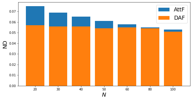
The results of the synthetic experiments on the cold-start and few-shot problems in Table 1 demonstrate that the performance of DAF is better than or on par with the baselines in all experiments. We also note the following observations to provide a better understanding into domain adaptation methods. First, we see that the cross-domain forecasters RDA and DAF that are jointly trained end-to-end using both source and target data are overall more accurate than the single-domain forecasters. This finding indicates that source data is helpful in forecasting the target data. Second, among the cross-domain forecasters DATSING is outperformed by RDA and DAF, indicating the importance of joint training on both domains. Third, on a majority of the experiments our attention-based DAF model is more accurate than or competitive to the RNN-based DA (RDA) method. We show the results for RDA-ADDA as the other DA variants, DANN and MMD, have similar performance. They are considered in the following real-world experiments (see Table 2). Finally, we observe in Figure 5 that DAF improves more significantly as the number of training samples becomes smaller.

5.3 Real-World Datasets

${\mathcal{D}}_{{\mathcal{T}}}$	${\mathcal{D}}_{{\mathcal{S}}}$	$\tau$	DAR	AttF	SASA	DATSING	RDA-DANN	RDA-ADDA	RDA-MMD	DAF
traf	elec	24	0.205 $\pm$ 0.015	0.182 $\pm$ 0.007	0.177 $\pm$ 0.004	0.184 $\pm$ 0.004	0.181 $\pm$ 0.009	0.174 $\pm$ 0.005	0.186 $\pm$ 0.004	0.169 $\pm$ 0.002
traf	wiki		0.205 $\pm$ 0.015	0.182 $\pm$ 0.007	0.197 $\pm$ 0.001	0.189 $\pm$ 0.005	0.180 $\pm$ 0.004	0.181 $\pm$ 0.003	0.179 $\pm$ 0.004	0.176 $\pm$ 0.004
elec	traf		0.141 $\pm$ 0.023	0.137 $\pm$ 0.005	0.164 $\pm$ 0.001	0.137 $\pm$ 0.003	0.133 $\pm$ 0.005	0.134 $\pm$ 0.002	0.140 $\pm$ 0.006	0.125 $\pm$ 0.008
elec	sales		0.141 $\pm$ 0.023	0.137 $\pm$ 0.005	0.160 $\pm$ 0.001	0.149 $\pm$ 0.009	0.135 $\pm$ 0.007	0.142 $\pm$ 0.003	0.144 $\pm$ 0.003	0.123 $\pm$ 0.005
wiki	traf	7	0.055 $\pm$ 0.010	0.050 $\pm$ 0.003	0.053 $\pm$ 0.001	0.049 $\pm$ 0.002	0.047 $\pm$ 0.005	0.045 $\pm$ 0.003	0.045 $\pm$ 0.003	0.042 $\pm$ 0.004
wiki	sales		0.055 $\pm$ 0.010	0.050 $\pm$ 0.003	0.053 $\pm$ 0.001	0.052 $\pm$ 0.004	0.053 $\pm$ 0.002	0.049 $\pm$ 0.003	0.052 $\pm$ 0.004	0.049 $\pm$ 0.003
sales	elec		0.305 $\pm$ 0.005	0.308 $\pm$ 0.002	0.451 $\pm$ 0.001	0.301 $\pm$ 0.008	0.297 $\pm$ 0.004	0.281 $\pm$ 0.001	0.291 $\pm$ 0.004	0.277 $\pm$ 0.005
sales	wiki		0.305 $\pm$ 0.005	0.308 $\pm$ 0.002	0.301 $\pm$ 0.001	0.305 $\pm$ 0.008	0.287 $\pm$ 0.009	0.287 $\pm$ 0.002	0.289 $\pm$ 0.003	0.280 $\pm$ 0.007

Table 2: Performance comparison of DAF on real-world benchmark datasets with prediction length

\tau

in the target domain in terms of the mean +/- standard deviation ND metric. The winners and the competitive followers (the gap is smaller than its standard deviation over 5 runs) are bolded for reference.

We perform experiments on four real benchmark datasets that are widely used in forecasting literature: elec and traf from the UCI data repository (Dua & Graff, 2017), sales (Kar, 2019) and wiki (Lai, 2017) from Kaggle. Notably, the elec and traf datasets present clear daily and weekly patterns while sales and wiki are less regular and more challenging. We use the following time features $\xi_{t}\in\mathbb{R}^{2}$ as covariates: the day of the week and hour of the day for the hourly datasets elec and traf, and the day of the month and day of the week for the daily datasets sales and wiki. For more dataset details, see appendix A.

To evaluate the performance of DAF, we consider cross-dataset adaptation, i.e., transferring between a pair of datasets. Since the original datasets are large enough to train a reasonably good forecaster, we only take a subset of each dataset as a target domain to simulate the data-scarce situation. Specifically, we take the last $30$ days of each time series in the hourly dataset elec and traf, and the last $60$ days from daily dataset sales and wiki. We partition the target datasets equally into training/validation/test splits, i.e. $10/10/10$ days for hourly datasets and $20/20/20$ days for daily datasets. The full datasets are used as source domains in adaptation. We follow the rolling window strategy from Flunkert et al. (2020), and split each window into historical and prediction time series of lengths $T$ and $T+\tau$ , respectively. In our experiments, we set $T=168,\tau=24$ for hourly datasets, and $T=28,\tau=7$ for the daily datasets. For DA methods, the splitting of the source data follows analogously.

Table 2 shows that the conclusions drawn from Table 1 on the synthetic experiments generally hold on the real-world datasets. In particular, we see the accuracy improvement by DAF over the baselines is more significant than that in the synthetic experiments. The real-world experiments also demonstrate that in general the success of DAF is agnostic of the source domain, and is even effective when transferring from a source domain of different frequency than that of the target domain. In addition, the cross-domain forecasters, DATSING, the RDA variants and our DAF outperform the three single-domain baselines in most cases. As in the synthetic cases, DATSING performs relatively worse than RDA and DAF. On the other hand, another cross-domain forecaster SASA is originally designed for regression tasks, where a fixed-sized window is used to predict a single exogeneous numerical label. While it can be extended to multi-horizon forecasting tasks by replacing the label with the next-step value and making autoregressive predictions, the performance is significantly worse than other cross-domain competitors and even some single-domain counterparts in some cases. The accuracy differences between DAF and RDA are larger than in the synthetic case, and in favor of DAF. This finding further demonstrates that our choice of an attention-based architecture is well-suited for real domain adaptation problems.

Remarkably, DAF manages to learn the different patterns between source and target domains under our setups. For instance, Figure 6 illustrates that DAF can successfully learn clear daily patterns in the traf dataset, and find irregular patterns in the sales dataset. A reason for its success is that the private encoders capture features at various scales in different domains, and the attention module captures domain-dependent patterns by context matching using domain-invariant queries and keys.

${\mathcal{D}}_{\mathcal{T}}$	${\mathcal{D}}_{\mathcal{S}}$	$\tau$	no-adv	no- $q$ -share	no- $k$ -share	$v$ -share	DAF
traf	elec	24	0.172	0.171	0.172	0.176	0.168
elec	traf	24	0.121	0.122	0.120	0.127	0.119
wiki	sales	7	0.042	0.042	0.044	0.049	0.041
sales	wiki	7	0.294	0.283	0.282	0.291	0.280

Table 3: Results of ablation studies of DAF variants on four adaptation tasks on real-world datasets.

5.4 Additional Experiments

In addition to the listed baselines in section 5.1, we also compare DAF with other single-domain forecasters, e.g. ConvTrans (Li et al., 2019), N-BEATS (Oreshkin et al., 2020b), and domain adaptation methods on time series tasks, e.g. MetaF (Oreshkin et al., 2020a). These methods are either similar to the baselines in Table 2 or designed for a different setting. We still adapt them to our setting to provide additional results in Tables 6-7 in appendix C.

5.5 Ablation Studies

In order to examine the effectiveness of our designs, we conduct ablation studies by adjusting each key component successively. Table 3 shows the improved performance of DAF over its variants on the target domain on four adaptation tasks. Equipped with a domain discriminator, DAF improves its effectiveness of adaptation compared to its non-adversarial variant (no-adv). We see that sharing both keys and queries in DAF results in performance gains over not sharing either (no- $k$ -share and no- $q$ -share). Furthermore, it is clear that our design choice of the values to be domain-specific for domain-dependent forecasts rather than shared ( $v$ -share) has the largest positive impact on the performance.

Figure 7 visualizes the distribution of queries and keys learned by DAF and no-adv, where the target data ${\mathcal{D}}_{{\mathcal{T}}}=\textit{traf}$ and the source data ${\mathcal{D}}_{{\mathcal{S}}}=\textit{elec}$ via a TSNE embedding. Empirically, we see the latent distributions are well aligned in DAF and not in no-adv. This can explain the improved performance of DAF over its variants. It also further verifies our intuition that DAF benefits from an aligned latent space of queries and keys across domains.

6 Conclusions

In this paper, we aim to apply domain adaptation to time series forecasting to solve the data scarcity problem. We identify the differences between the forecasting task and common domain adaptation scenarios, and accordingly propose the Domain Adaptation Forecaster (DAF) based on attention sharing. Through empirical experiments, we demonstrate that DAF outperforms state-of-the-art single-domain forecasters and various domain adaptation baselines on synthetic and real-world datasets. We further show the effectiveness of our designs via extensive ablation studies. In spite of empirical evidences, the theoretical justification of having domain-invariant features within attention models remains an open problem. Extension to multi-variate time series forecasting experiments is another direction of future work.

References

Alam et al. (2018) Alam, F., Joty, S., and Imran, M. Domain Adaptation with Adversarial Training and Graph Embeddings. In Proceedings of the 56th Annual Meeting of the Association for Computational Linguistics (Volume 1: Long Papers), pp. 1077–1087, Melbourne, Australia, 2018. Association for Computational Linguistics. doi: 10.18653/v1/P18-1099. URL http://aclweb.org/anthology/P18-1099.
Bartunov & Vetrov (2018) Bartunov, S. and Vetrov, D. P. Few-shot Generative Modelling with Generative Matching Networks. International Conference on Artificial Intelligence and Statistics, pp. 670–678, 2018.
Ben-David et al. (2010) Ben-David, S., Blitzer, J., Crammer, K., Kulesza, A., Pereira, F., and Vaughan, J. W. A theory of learning from different domains. Machine Learning, 79(1-2):151–175, May 2010. ISSN 0885-6125, 1573-0565. doi: 10.1007/s10994-009-5152-4. URL http://link.springer.com/10.1007/s10994-009-5152-4.
Borovykh et al. (2017) Borovykh, A., Bohte, S., and Oosterlee, C. W. Conditional time series forecasting with convolutional neural networks. arXiv preprint arXiv:1703.04691, 2017.
Böse et al. (2017) Böse, J.-H., Flunkert, V., Gasthaus, J., Januschowski, T., Lange, D., Salinas, D., Schelter, S., Seeger, M., and Wang, Y. Probabilistic demand forecasting at scale. Proceedings of the VLDB Endowment, 10(12):1694–1705, 2017.
Bousmalis et al. (2016) Bousmalis, K., Trigeorgis, G., Silberman, N., Krishnan, D., and Erhan, D. Domain Separation Networks. volume 29, pp. 345–351, 2016.
Cai et al. (2021) Cai, R., Chen, J., Li, Z., Chen, W., Zhang, K., Ye, J., Li, Z., Yang, X., and Zhang, Z. Time Series Domain Adaptation via Sparse Associative Structure Alignment. Proceedings of the AAAI Conference on Artificial Intelligence, 35:6859–6867, 2021.
Chen et al. (2020) Chen, W.-Y., Liu, Y.-C., Kira, Z., Wang, Y.-C. F., and Huang, J.-B. A Closer Look at Few-shot Classification. arXiv:1904.04232 [cs], January 2020. URL http://arxiv.org/abs/1904.04232. arXiv: 1904.04232.
Cortes & Mohri (2011) Cortes, C. and Mohri, M. Domain Adaptation in Regression. In Kivinen, J., Szepesvári, C., Ukkonen, E., and Zeugmann, T. (eds.), Algorithmic Learning Theory, volume 6925, pp. 308–323. Springer Berlin Heidelberg, Berlin, Heidelberg, 2011. ISBN 978-3-642-24411-7 978-3-642-24412-4. doi: 10.1007/978-3-642-24412-4˙25. URL http://link.springer.com/10.1007/978-3-642-24412-4_25. Series Title: Lecture Notes in Computer Science.
Cuturi & Blondel (2017) Cuturi, M. and Blondel, M. Soft-DTW: a Differentiable Loss Function for Time-Series. arXiv:1703.01541 [stat], March 2017. URL http://arxiv.org/abs/1703.01541. arXiv: 1703.01541.
Devlin et al. (2019) Devlin, J., Chang, M.-W., Lee, K., and Toutanova, K. BERT: Pre-training of Deep Bidirectional Transformers for Language Understanding. In Proceedings of the 2019 Conference of the North American Chapter of the Association for Computational Linguistics: Human Language Technologies, Volume 1 (Long and Short Papers), pp. 4171–4186, 2019. URL http://arxiv.org/abs/1810.04805. arXiv: 1810.04805.
Dua & Graff (2017) Dua, D. and Graff, C. UCI Machine Learning Repository. University of California, Irvine, School of Information and Computer Sciences, 2017. URL http://archive.ics.uci.edu/ml.
Flunkert et al. (2020) Flunkert, V., Salinas, D., and Gasthaus, J. DeepAR: Probabilistic Forecasting with Autoregressive Recurrent Networks. International Journal of Forecasting, 36:1181–1191, 2020. arXiv: 1704.04110.
Ganin & Lempitsky (2015) Ganin, Y. and Lempitsky, V. Unsupervised Domain Adaptation by Backpropagation. International conference on machine learning, pp. 1180–1189, 2015.
Ganin et al. (2016) Ganin, Y., Ustinova, E., Ajakan, H., Germain, P., Larochelle, H., Laviolette, F., Marchand, M., and Lempitsky, V. Domain-Adversarial Training of Neural Networks. The journal of machine learning research, 17:2096–2030, 2016.
Ghifary et al. (2016) Ghifary, M., Kleijn, W. B., Zhang, M., Balduzzi, D., and Li, W. Deep Reconstruction-Classification Networks for Unsupervised Domain Adaptation. In European conference on computer vision, pp. 597–613, 2016.
Guo et al. (2020) Guo, H., Pasunuru, R., and Bansal, M. Multi-Source Domain Adaptation for Text Classification via DistanceNet-Bandits. Proceedings of the AAAI Conference on Artificial Intelligence, 34(05):7830–7838, April 2020. ISSN 2374-3468, 2159-5399. doi: 10.1609/aaai.v34i05.6288. URL https://aaai.org/ojs/index.php/AAAI/article/view/6288.
Gururangan et al. (2020) Gururangan, S., Marasović, A., Swayamdipta, S., Lo, K., Beltagy, I., Downey, D., and Smith, N. A. Don’t Stop Pretraining: Adapt Language Models to Domains and Tasks. In Proceedings of the 58th Annual Meeting of the Association for Computational Linguistics, pp. 8342–8360, Online, 2020. Association for Computational Linguistics. doi: 10.18653/v1/2020.acl-main.740. URL https://www.aclweb.org/anthology/2020.acl-main.740.
Han & Eisenstein (2019) Han, X. and Eisenstein, J. Unsupervised Domain Adaptation of Contextualized Embeddings for Sequence Labeling. In Proceedings of the 2019 Conference on Empirical Methods in Natural Language Processing and the 9th International Joint Conference on Natural Language Processing (EMNLP-IJCNLP), pp. 4237–4247, Hong Kong, China, 2019. Association for Computational Linguistics. doi: 10.18653/v1/D19-1433. URL https://www.aclweb.org/anthology/D19-1433.
Hoffman et al. (2018) Hoffman, J., Tzeng, E., Park, T., Zhu, J.-Y., Isola, P., Saenko, K., Efros, A. A., and Darrell, T. CyCADA: Cycle-Consistent Adversarial Domain Adaptation. International conference on machine learning, pp. 1989–1998, 2018.
Hu et al. (2020) Hu, H., Tang, M., and Bai, C. DATSING: Data Augmented Time Series Forecasting with Adversarial Domain Adaptation. In Proceedings of the 29th ACM International Conference on Information & Knowledge Management, pp. 2061–2064, Virtual Event Ireland, October 2020. ACM. ISBN 978-1-4503-6859-9. doi: 10.1145/3340531.3412155. URL https://dl.acm.org/doi/10.1145/3340531.3412155.
Kan et al. (2022) Kan, K., Aubet, F.-X., Januschowski, T., Park, Y., Benidis, K., Ruthotto, L., and Gasthaus, J. Multivariate quantile function forecaster. In International Conference on Artificial Intelligence and Statistics, pp. 10603–10621. PMLR, 2022.
Kar (2019) Kar, P. Dataset of Kaggle Competition Rossmann Store Sales, version 2, January 2019. URL https://www.kaggle.com/pratyushakar/rossmann-store-sales.
Kim et al. (2020) Kim, J., Park, Y., Fox, J. D., Boyd, S. P., and Dally, W. Optimal operation of a plug-in hybrid vehicle with battery thermal and degradation model. In 2020 American Control Conference (ACC), pp. 3083–3090. IEEE, 2020.
Lai (2017) Lai. Dataset of Kaggle Competition Web Traffic Time Series Forecasting, Version 3, August 2017. URL https://www.kaggle.com/ymlai87416/wiktraffictimeseriesforecast/metadata.
Li et al. (2017) Li, C.-L., Chang, W.-C., Cheng, Y., Yang, Y., and Póczos, B. MMD GAN: towards deeper understanding of moment matching network. In Proceedings of the 31st International Conference on Neural Information Processing Systems, pp. 2200–2210, 2017.
Li et al. (2019) Li, S., Jin, X., Xuan, Y., Zhou, X., Chen, W., Wang, Y.-X., and Yan, X. Enhancing the Locality and Breaking the Memory Bottleneck of Transformer on Time Series Forecasting. Advances in Neural Information Processing Systems, pp. 5243–5253, 2019.
Liberty et al. (2020) Liberty, E., Karnin, Z., Xiang, B., Rouesnel, L., Coskun, B., Nallapati, R., Delgado, J., Sadoughi, A., Astashonok, Y., Das, P., Balioglu, C., Chakravarty, S., Jha, M., Gautier, P., Arpin, D., Januschowski, T., Flunkert, V., Wang, Y., Gasthaus, J., Stella, L., Rangapuram, S., Salinas, D., Schelter, S., and Smola, A. Elastic Machine Learning Algorithms in Amazon SageMaker. In Proceedings of the 2020 ACM SIGMOD International Conference on Management of Data, pp. 731–737, Portland OR USA, June 2020. ACM. ISBN 978-1-4503-6735-6. doi: 10.1145/3318464.3386126. URL https://dl.acm.org/doi/10.1145/3318464.3386126.
Lim et al. (2019) Lim, B., Arik, S. O., Loeff, N., and Pfister, T. Temporal Fusion Transformers for Interpretable Multi-horizon Time Series Forecasting. arXiv:1912.09363 [cs, stat], December 2019. URL http://arxiv.org/abs/1912.09363. arXiv: 1912.09363.
Long et al. (2015) Long, M., Cao, Y., Wang, J., and Jordan, M. I. Learning Transferable Features with Deep Adaptation Networks. pp. 97–105, 2015. URL http://arxiv.org/abs/1502.02791. arXiv: 1502.02791.
Motiian et al. (2017) Motiian, S., Jones, Q., Iranmanesh, S. M., and Doretto, G. Few-Shot Adversarial Domain Adaptation. Advances in Neural Information Processing Systems, pp. 6670–6680, 2017. URL http://arxiv.org/abs/1711.02536. arXiv: 1711.02536.
Oreshkin et al. (2020a) Oreshkin, B. N., Carpov, D., Chapados, N., and Bengio, Y. Meta-learning framework with applications to zero-shot time-series forecasting. arXiv:2002.02887 [cs, stat], February 2020a. URL http://arxiv.org/abs/2002.02887. arXiv: 2002.02887.
Oreshkin et al. (2020b) Oreshkin, B. N., Chapados, N., Carpov, D., and Bengio, Y. N-BEATS: Neural basis expansion analysis for interpretable time series forecasting. International Conference on Learning Representations, pp. 31, 2020b.
Park et al. (2019) Park, Y., Mahadik, K., Rossi, R. A., Wu, G., and Zhao, H. Linear quadratic regulator for resource-efficient cloud services. In Proceedings of the ACM Symposium on Cloud Computing, pp. 488–489, 2019.
Park et al. (2022) Park, Y., Maddix, D., Aubet, F.-X., Kan, K., Gasthaus, J., and Wang, Y. Learning quantile functions without quantile crossing for distribution-free time series forecasting. In International Conference on Artificial Intelligence and Statistics, pp. 8127–8150. PMLR, 2022.
Paszke et al. (2019) Paszke, A., Gross, S., Massa, F., Lerer, A., Bradbury, J., Chanan, G., Killeen, T., Lin, Z., Gimelshein, N., Antiga, L., Desmaison, A., Kopf, A., Yang, E., DeVito, Z., Raison, M., Tejani, A., Chilamkurthy, S., Steiner, B., Fang, L., Bai, J., and Chintala, S. PyTorch: An Imperative Style, High-Performance Deep Learning Library. Advances in neural information processing systems, pp. 8026–8037, 2019.
Purushotham et al. (2017) Purushotham, S., Carvalho, W., Nilanon, T., and Liu, Y. Variational Recurrent Adversarial Deep Domain Adaptation. In 5th International Conference on Learning Representations, ICLR 2017, Toulon, France, April 24-26, 2017, Conference Track Proceedings. OpenReview.net, 2017. URL https://openreview.net/forum?id=rk9eAFcxg.
Ramponi & Plank (2020) Ramponi, A. and Plank, B. Neural Unsupervised Domain Adaptation in NLP—A Survey. arXiv:2006.00632 [cs], May 2020. URL http://arxiv.org/abs/2006.00632. arXiv: 2006.00632.
Rangapuram et al. (2018) Rangapuram, S. S., Seeger, M., Gasthaus, J., Stella, L., Wang, Y., and Januschowski, T. Deep State Space Models for Time Series Forecasting. In Advances in neural information processing systems, pp. 7785–7794, 2018.
Rietzler et al. (2020) Rietzler, A., Stabinger, S., Opitz, P., and Engl, S. Adapt or Get Left Behind: Domain Adaptation through BERT Language Model Finetuning for Aspect-Target Sentiment Classification. Proceedings of The 12th Language Resources and Evaluation Conference, pp. 4933–4941, 2020.
Sen et al. (2019) Sen, R., Yu, H.-F., and Dhillon, I. Think Globally, Act Locally: A Deep Neural Network Approach to High-Dimensional Time Series Forecasting. Advances in Neural Information Processing Systems, 32, 2019.
Shi et al. (2018) Shi, G., Feng, C., Huang, L., Zhang, B., Ji, H., Liao, L., and Huang, H. Genre Separation Network with Adversarial Training for Cross-genre Relation Extraction. In Proceedings of the 2018 Conference on Empirical Methods in Natural Language Processing, pp. 1018–1023, Brussels, Belgium, 2018. Association for Computational Linguistics. doi: 10.18653/v1/D18-1125. URL http://aclweb.org/anthology/D18-1125.
Tzeng et al. (2017) Tzeng, E., Hoffman, J., Saenko, K., and Darrell, T. Adversarial Discriminative Domain Adaptation. In 2017 IEEE Conference on Computer Vision and Pattern Recognition (CVPR), pp. 2962–2971, Honolulu, HI, July 2017. IEEE. ISBN 978-1-5386-0457-1. doi: 10.1109/CVPR.2017.316. URL http://ieeexplore.ieee.org/document/8099799/.
Vaswani et al. (2017) Vaswani, A., Shazeer, N., Parmar, N., Uszkoreit, J., Jones, L., Gomez, A. N., Kaiser, L., and Polosukhin, I. Attention Is All You Need. In Advances in neural information processing systems, pp. 5998–6008, 2017.
Wang et al. (2020) Wang, H., He, H., and Katabi, D. Continuously indexed domain adaptation. In ICML, 2020.
Wang et al. (2021) Wang, R., Maddix, D., Faloutsos, C., Wang, Y., and Yu, R. Bridging Physics-based and Data-driven modeling for Learning Dynamical Systems. In Learning for Dynamics and Control, pp. 385–398, 2021.
Wang et al. (2005) Wang, W., Van Gelder, P. H., and Vrijling, J. Some issues about the generalization of neural networks for time series prediction. In International Conference on Artificial Neural Networks, pp. 559–564. Springer, 2005.
Wang et al. (2019) Wang, Y., Smola, A., Maddix, D. C., Gasthaus, J., Foster, D., and Januschowski, T. Deep Factors for Forecasting. In International conference on machine learning, pp. 6607–6617, 2019.
Wen et al. (2017) Wen, R., Torkkola, K., Narayanaswamy, B., and Madeka, D. A Multi-Horizon Quantile Recurrent Forecaster. arXiv:1711.11053 [stat], November 2017. URL http://arxiv.org/abs/1711.11053. arXiv: 1711.11053.
Wilson & Cook (2020) Wilson, G. and Cook, D. J. A Survey of Unsupervised Deep Domain Adaptation. arXiv:1812.02849 [cs, stat], February 2020. URL http://arxiv.org/abs/1812.02849. arXiv: 1812.02849.
Wilson et al. (2020) Wilson, G., Doppa, J. R., and Cook, D. J. Multi-Source Deep Domain Adaptation with Weak Supervision for Time-Series Sensor Data. In Proceedings of the 26th ACM SIGKDD International Conference on Knowledge Discovery & Data Mining, pp. 1768–1778, Virtual Event CA USA, August 2020. ACM. ISBN 978-1-4503-7998-4. doi: 10.1145/3394486.3403228. URL https://dl.acm.org/doi/10.1145/3394486.3403228.
Wright & Augenstein (2020) Wright, D. and Augenstein, I. Transformer Based Multi-Source Domain Adaptation. In Proceedings of the 2020 Conference on Empirical Methods in Natural Language Processing (EMNLP), pp. 7963–7974, Online, 2020. Association for Computational Linguistics. doi: 10.18653/v1/2020.emnlp-main.639. URL https://www.aclweb.org/anthology/2020.emnlp-main.639.
Wu et al. (2020) Wu, S., Xiao, X., Ding, Q., Zhao, P., Wei, Y., and Huang, J. Adversarial Sparse Transformer for Time Series Forecasting. Advances in Neural Information Processing Systems, 33:11, 2020.
Xu et al. (2021) Xu, J., Wang, J., Long, M., and others. Autoformer: Decomposition transformers with auto-correlation for long-term series forecasting. Advances in Neural Information Processing Systems, 34, 2021.
Xu et al. (2022) Xu, Z., Lee, G.-H., Wang, Y., Wang, H., et al. Graph-relational domain adaptation. ICLR, 2022.
Yao et al. (2020) Yao, Z., Wang, Y., Long, M., and Wang, J. Unsupervised transfer learning for spatiotemporal predictive networks. In International Conference on Machine Learning, pp. 10778–10788. PMLR, 2020.
Yoon et al. (2022) Yoon, T., Park, Y., Ryu, E. K., and Wang, Y. Robust probabilistic time series forecasting. arXiv preprint arXiv:2202.11910, 2022.
Yu et al. (2016) Yu, H.-F., Rao, N., and Dhillon, I. S. Temporal Regularized Matrix Factorization for High-dimensional Time Series Prediction. NIPS, pp. 847–855, 2016.
Zhao et al. (2018) Zhao, H., Zhang, S., Wu, G., Moura, J. M. F., Costeira, J. P., and Gordon, G. J. Adversarial Multiple Source Domain Adaptation. Advances in neural information processing systems, pp. 8559–8570, 2018.
Zhou et al. (2021) Zhou, H., Zhang, S., Peng, J., Zhang, S., Li, J., Xiong, H., and Zhang, W. Informer: Beyond Efficient Transformer for Long Sequence Time-Series Forecasting. In Proceedings of the AAAI Conference on Artificial Intelligence, 2021. URL http://arxiv.org/abs/2012.07436. arXiv: 2012.07436.

Appendix A Dataset Details

A.1 Synthetic Datasets

The synthetic datasets consist of sinusoidal signals with uniformly sampled parameters as follows:

	$\displaystyle z_{i,t}$	$\displaystyle=A_{i}\sin(2\pi\omega_{i}t+\phi_{i})+c_{i}+\epsilon_{i,t},\quad t\in[0,T+\tau],$
	$\displaystyle A_{i}$	$\displaystyle\sim\text{Unif}(A_{\min},A_{\max}),\quad c_{i}\sim\text{Unif}(c_{\min},c_{\max}),$
	$\displaystyle\omega_{i}$	$\displaystyle\sim\text{Unif}(\omega_{\min},\omega_{\max}),\quad\phi_{i}\sim\text{Unif}(-2\pi,2\pi),$

where $A_{\min},A_{\max}\in\mathbb{R}^{+}$ denote the amplitudes, $c_{\min},c_{\max}\in\mathbb{R}$ denote the levels, and $\omega_{\min},\omega_{\max}\in[\frac{1}{T},\frac{20}{T}]$ denote the frequencies. In addition, $\epsilon_{i,t}\sim{\mathcal{N}}(0,0.2)$ is a white noise term. In our experiments, we fix $T=144,\tau=18,A_{\min}=0.5,A_{\max}=5.0$ , $c_{\min}=-3.0,c_{\max}=3.0$ .

A.2 Real-World Datasets

Table 4 summarizes the four benchmark real-world datasets that we use to evaluate our DAF model.

Dataset

Freq

Value

# Time

Series

Average

Length

Comment

elec

hourly

\mathbb{R}^{+}

370

3304

Household

electricity

consumption

traf

hourly

[0,1]

963

360

Occupancy rate

of SF Bay Area

highways

sales

daily

\mathbb{N}^{+}

500

1106

Daily sales of

Rossmann

grocery stores

wiki

daily

\mathbb{N}^{+}

9906

Visit counts of

various Wikipedia

pages

Table 4: Benchmark dataset descriptions.

For evaluation, we follow Flunkert et al. (2020), and we take moving windows of length $T+\tau$ starting at different points from the original time series in the datasets. For an original time series $[z_{i,t}]_{t=1}^{L}$ of length $L$ , we obtain a set of moving windows:

\{[z_{i,t}]_{t=n}^{n+T+\tau-1},\qquad n=1,2,\dots,L-T-\tau+1\}.

This procedure results in a set of fixed-length trajectory samples. Each sample is further split into historical observations $X$ and forecasting targets $Y$ , where the lengths of $X$ and $Y$ are $T$ and $\tau$ , respectively. We randomly select samples from the population by uniform sampling for training, validation and test sets.

Appendix B Implementation Details

B.1 Baselines

In this subsection, we provide an overview of the following baseline models, including conventional single-domain forecasters trained only on the target domain:

•

DeepAR (DAR): auto-regressive RNN-based model with LSTM units (we directly call DeepAR implemented by Amazon Sagemaker);
•

Vanilla Transformer (VT): sequence-to-sequence model based on common transformer architecture;
•

ConvTrans (CT): attention-based forecaster that builds attention blocks on convolutional activations as DAF does. Unlike DAF, it does not reconstruct the input, and only fits the future. From a probabilistic perspective, it models the conditional distribution $P(Y|X)$ instead of the joint distribution $P(X,Y)$ as DAF does, where $X$ and $Y$ are history and future, respective. In addition, it directly uses the outputs of the convolution as queries and keys in the attention module;
•

AttF: single-domain version of DAF. It is equivalent to the branch of the sequence generator for the target domain in DAF. It has access to the attention module, but does not share it with another branch;
•

N-BEATS: MLP-based forecaster. Similar to DAF, it aims to forecast the future as well as to reconstruct the given history. N-BEATS only consumes univariate time series $z_{i,t}$ , and does not accept covariates $\xi_{i,t}$ as input. In the original paper Oreshkin et al. (2020b), it employs various objectives and ensembles to improve the results. In our implementation, we use the ND metric as the training objective, and do not use any ensembling techniques for a fair comparison;

and cross-domain forecasters trained on both source and target domain:

•

MetaF: method with the same architecture as N-BEATS. It trains a model on the source dataset, and applies it to the target dataset in a zero-shot setting, i.e. without any fine-tuning. Both MetaF and N-BEATS rely on given Fourier bases to fit seasonal patterns. For instance, bases of period 24 and 168 are included for hourly datasets, whereas bases of period 7 are included for daily datasets. The daily and weekly patterns are expected to be captured in all settings.
•

PreTrained Forecaster (PTF): method with the same architecture as AttF for the target data. Unlike AttF, PTF fits both source and target data. It is first pretrained on the source dataset, and then finetuned on the target dataset.
•

SASA: Cai et al. (2021) is another related work that we introduce in section 2, which focuses on time series classification and regression tasks, where a single exogenous label instead of a sequence of future values is predicted. We replace the original labels of the regression task with the next value of the respective time series, and autoregressively predicting the next step for multi-horizon forecasting. In the experiments, we revise the official code ¹¹1https://github.com/DMIRLAB-Group/SASA. accordingly and keep the provided default hyperparameters.
•

DATSING: a forecasting framework based on NBEATS (Oreshkin et al., 2020b) architecture. The model is first pre-trained on the source dataset. Then a subset of source data that includes nearest neighbors to a target sample in terms of soft-DTW (Cuturi & Blondel, 2017) is selected to fine-tune the pre-trained model before it is evaluated using the respective target sample. During fine-tuning, a domain discriminator is used to distinguish the nearest neighbors from the same number of source samples drawn from the complement set.
•
RDA has the same overall structure as DAF, but replaces the attention module in DAF with a LSTM module. The encoder module produces a single encoding, which is then consumed by the MLP-based decoder. We take three traditional methods for domain adaptation:
- –
  
  RDA-DANN: The encoder and decoder are shared across domains. The sequence generator is trained to fit data from both domains. Meanwhile, the gradient of domain discriminator will be reversed before back-propagated to the encoder.
- –
  
  RDA-ADDF: The encoder and decoder are not shared across domains. During training, the source encoder and decoder are first trained to fit source data. Then encodings from both encoders are discriminated by the domain discriminator with the source encoder parameters frozen. Finally, the target encoder and decoder are trained to fit target data with the target encoder parameters frozen.
- –
  
  RDA-MMD: Instead of a domain discriminators, the Maximum Mean Discrepancy between source and target encodings is optimized with the sequence generators.

B.2 Hyperparameters

The following hyperparameters of DAF and baseline models are selected by grid-search over the validation set:

•

the hidden dimension $h\in\{32,64,128,256\}$ of all models;
•

the number of MLP layers $l_{\text{MLP}}\in\{4\}$ for N-BEATS ²²2We set the other hyperparameters for N-BEATS as suggested in the original paper Oreshkin et al. (2020b)., $l_{\text{MLP}}\in\{1,2,3\}$ for AttF, DAF and its variants;
•

the number of RNN layers $l_{\text{RNN}}\in\{1,3\}$ in DAR and RDA;
•

the kernel sizes of convolutions $s\in\{3,13,(3,5),(3,17)\}$ in AttF, DAF and its variants; ³³3A single integer means a single convolution layer in the encoder module, while a tuple stands for multiple convolutions.
•

the learning rate $\gamma\in\{0.001,0.01,0.1\}$ for all models;
•

the trade-off coefficient $\lambda\in\{0.1,1,10\}$ in equation (2) for DAF, RDA-ADDA;
•

In RDA-MMD, the factor of the MMD item in the objective selected from $\{0.1,1.0,10.0\}$ .

For RDA-DANN, we set a schedule

\lambda=\frac{2}{1+\exp(-10e/E)}-1,

where $e$ denotes the current epoch and $E$ denotes the total number of epochs for the factor $\lambda$ of the reversed gradient from the domain discriminator according to Ganin et al. (2016).

Table 5 summarizes the specific configurations of the hyper-parameters for our proposed DAF model in the experiments.

	$h$	$l_{\text{MLP}}$	$s$	$\gamma$	$\lambda$
cold-start	64	1	(3,5)	1e-3	1.0
few-shot	64	1	(3,5)	1e-3	1.0
elec	128	1	13	1e-3	1.0
traf	64	1	(3,17)	1e-2	10.0
wiki	64	2	(3,5)	1e-3	1.0
sales	128	2	(3,5)	1e-3	1.0

Table 5: Hyperparameters of DAF models in various synthetic and real-world experiments.

The models are trained for at most $100K$ iterations, which we empirically find to be more than sufficient for the models to converge. We use early stopping with respect to the ND metric on the validation set.

Appendix C Detailed Experiment Results

Task	Cold-start			Few-shot
$N$	5000			20	50	100
$T$	36	45	54	144
$\tau$	18
DeepAR	0.053 $\pm$ 0.003	0.037 $\pm$ 0.002	0.031 $\pm$ 0.002	0.062 $\pm$ 0.003	0.059 $\pm$ 0.004	0.059 $\pm$ 0.003
N-BEATS	0.044 $\pm$ 0.001	0.044 $\pm$ 0.001	0.042 $\pm$ 0.001	0.079 $\pm$ 0.001	0.060 $\pm$ 0.001	0.054 $\pm$ 0.002
CT	0.042 $\pm$ 0.001	0.041 $\pm$ 0.004	0.038 $\pm$ 0.005	0.095 $\pm$ 0.003	0.074 $\pm$ 0.005	0.071 $\pm$ 0.002
AttF	0.042 $\pm$ 0.001	0.041 $\pm$ 0.004	0.038 $\pm$ 0.005	0.095 $\pm$ 0.003	0.074 $\pm$ 0.005	0.071 $\pm$ 0.002
MetaF	0.045 $\pm$ 0.005	0.043 $\pm$ 0.006	0.042 $\pm$ 0.002	0.071 $\pm$ 0.004	0.061 $\pm$ 0.003	0.053 $\pm$ 0.003
PTF	0.039 $\pm$ 0.006	0.037 $\pm$ 0.005	0.034 $\pm$ 0.008	0.086 $\pm$ 0.004	0.086 $\pm$ 0.003	0.081 $\pm$ 0.005
DATSING	0.039 $\pm$ 0.004	0.039 $\pm$ 0.002	0.037 $\pm$ 0.001	0.078 $\pm$ 0.005	0.076 $\pm$ 0.006	0.058 $\pm$ 0.005
RDA-ADDA	0.035 $\pm$ 0.002	0.034 $\pm$ 0.001	0.034 $\pm$ 0.001	0.059 $\pm$ 0.003	0.054 $\pm$ 0.003	0.053 $\pm$ 0.007
DAF	0.035 $\pm$ 0.003	0.030 $\pm$ 0.003	0.029 $\pm$ 0.003	0.057 $\pm$ 0.004	0.055 $\pm$ 0.001	0.051 $\pm$ 0.001

Table 6: Performance comparison of DAF to all baselines on synthetic datasets. The winners and the competitive followers (the gap is smaller than its standard deviation over 5 runs) are bolded for reference.

${\mathcal{D}}_{{\mathcal{T}}}$	traf		elec		wiki		sales
${\mathcal{D}}_{{\mathcal{S}}}$	elec	wiki	traf	sales	traf	sales	elec	wiki
DAR	0.205 $\pm$ 0.015		0.141 $\pm$ 0.023		0.055 $\pm$ 0.010		0.305 $\pm$ 0.005
N-BEATS	0.191 $\pm$ 0.003		0.147 $\pm$ 0.004		0.059 $\pm$ 0.008		0.299 $\pm$ 0.005
VT	0.187 $\pm$ 0.003		0.144 $\pm$ 0.004		0.061 $\pm$ 0.008		0.293 $\pm$ 0.005
CT	0.183 $\pm$ 0.013		0.131 $\pm$ 0.005		0.051 $\pm$ 0.006		0.324 $\pm$ 0.013
AttF	0.182 $\pm$ 0.007		0.137 $\pm$ 0.005		0.050 $\pm$ 0.003		0.308 $\pm$ 0.002
MetaF	0.190 $\pm$ 0.005	0.188 $\pm$ 0.002	0.151 $\pm$ 0.004	0.144 $\pm$ 0.004	0.061 $\pm$ 0.003	0.059 $\pm$ 0.005	0.311 $\pm$ 0.001	0.329 $\pm$ 0.002
PTF	0.184 $\pm$ 0.003	0.185 $\pm$ 0.004	0.144 $\pm$ 0.005	0.138 $\pm$ 0.007	0.044 $\pm$ 0.003	0.047 $\pm$ 0.002	0.287 $\pm$ 0.004	0.292 $\pm$ 0.007
DATSING	0.184 $\pm$ 0.004	0.189 $\pm$ 0.005	0.137 $\pm$ 0.003	0.149 $\pm$ 0.009	0.049 $\pm$ 0.002	0.052 $\pm$ 0.004	0.301 $\pm$ 0.008	0.305 $\pm$ 0.008
RDA-DANN	0.181 $\pm$ 0.009	0.180 $\pm$ 0.004	0.133 $\pm$ 0.005	0.135 $\pm$ 0.007	0.047 $\pm$ 0.005	0.053 $\pm$ 0.002	0.297 $\pm$ 0.004	0.287 $\pm$ 0.009
RDA-ADDA	0.174 $\pm$ 0.005	0.181 $\pm$ 0.003	0.134 $\pm$ 0.002	0.142 $\pm$ 0.003	0.045 $\pm$ 0.003	0.049 $\pm$ 0.003	0.281 $\pm$ 0.001	0.287 $\pm$ 0.002
RDA-MMD	0.186 $\pm$ 0.004	0.179 $\pm$ 0.004	0.140 $\pm$ 0.006	0.144 $\pm$ 0.003	0.045 $\pm$ 0.003	0.052 $\pm$ 0.004	0.291 $\pm$ 0.004	0.289 $\pm$ 0.003
DAF	0.169 $\pm$ 0.002	0.176 $\pm$ 0.004	0.125 $\pm$ 0.008	0.123 $\pm$ 0.005	0.042 $\pm$ 0.004	0.049 $\pm$ 0.003	0.277 $\pm$ 0.005	0.280 $\pm$ 0.007

Table 7: Performance comparison of DAF to all baselines on real-world benchmark datasets. The winners and the competitive followers (the gap is smaller than its standard deviation over 5 runs) are bolded for reference.

Tables 6-7 display a comprehensive comparison of DAF with all the aforementioned baselines on the synthetic and real-world data, respectively. As a conclusion, we see that DAF outperforms or is on par with the baselines in all cases with RDA-ADDA being the most competitive in some cases.

We also provide visualizations of forecasts for both synthetic and real-world experiments. Figure 8 provides more samples for the few-shot experiment where $N=20$ as a complement to Figure 4. We see that DAF is able to approximately capture the sinusoidal signals even if the input is contaminated by white noise in most cases, while AttF fails in many cases. Figure 9 illustrates the performance gap between DAF and AttF in the experiment with source data elec and target data traf as an example in real scenarios. While AttF generally captures daily patterns, DAF performs significantly better.