Does the structure of Pop III supernova ejecta affect the elemental abundance of extremely metal-poor stars?
Abstract
The first generation of metal-free (Pop III) stars are crucial for the production of heavy elements in the earliest phase of structure formation. Their mass scale can be derived from the elemental abundance pattern of extremely metal-poor (EMP) stars, which are assumed to inherit the abundances of uniformly mixed supernova (SN) ejecta. If the expanding ejecta maintains its initial stratified structure, the elemental abundance pattern of EMP stars might be different from that from uniform ejecta. In this work we perform numerical simulations of the metal enrichment from stratified ejecta for normal core-collapse SNe (CCSNe) with a progenitor mass and explosion energies 0.7–10 B (). We find that SN shells fall back into the central minihalo in all models. In the recollapsing clouds, the abundance ratio for stratified ejecta is different from the one for uniform ejecta only within dex for any element M. We also find that, for the largest explosion energy (10 B), a neighboring halo is also enriched. Only the outer layers containing Ca or lighter elements reach the halo, where . This means that C-enhanced metal-poor (CEMP) stars can form from the CCSN even with an average abundance ratio .
keywords:
galaxies: evolution — ISM: abundances — stars: formation — stars: low-mass — stars: Population III — stars: Population II1 INTRODUCTION
The first generation of metal-free (Population III; Pop III) stars enrich the early Universe with the first heavy elements, affecting later structure formation. Pop III stars form in dark matter halos with masses – (minihalos; MH) mainly at redshifts –30. If they are massive (), metals ejected from their supernova (SNe) can enhance star formation (e.g., Ritter et al., 2016). The efficiency of their feedback depends on stellar mass and SN explosion energy, which in turn change the luminosity and metal ejecta mass, respectively. Theoretical works suggest that Pop III stars are massive (–) because gas cooling caused by only molecular hydrogen is inefficient, and their parent clouds are stable against fragmentation (Bromm et al., 1999; Abel et al., 2002; Hirano et al., 2014; Susa et al., 2014). Although recent numerical studies have found that low-mass Pop III stars () can form through the fragmentation of accretion disks (e.g., Clark et al., 2011; Greif et al., 2012; Stacy & Bromm, 2014), we restrict our focus on massive stars to study their metal enrichment.
A number of previous works have attempted to constrain the mass of Pop III stars. One approach is to directly observe Pop III stars, but no metal-free stars have so far been found albeit the large survey programs of stars in the Milky Way and neighboring dwarf galaxies, such as the HK (Beers et al., 1985, 1992), Hamburg/ESO (Christlieb, 2003), SEGUE (Yanny et al., 2009), and LAMOST (Cui et al., 2012; Deng et al., 2012) surveys. The lower limit of iron abundance ,111The number abundance ratio of an element A to B is conventionally given with where is the absolute abundance defined as and is the number fraction of A relative to hydrogen nuclei. which is often used as a proxy to the stellar metallicity, of the stars ever observed is (; Caffau et al., 2011b) for carbon-normal stars. Some of the so-called carbon-enhanced metal-poor (CEMP) stars have even smaller fractions of Fe (), but they have enhanced carbon abundances (Beers & Christlieb, 2005; Aoki et al., 2007). Another approach is to measure the elemental abundance ratio of extremely metal-poor (EMP) stars with metallicities , which are considered to form from clouds enriched by a single or several Pop III SNe (Ryan et al., 1996; Cayrel et al., 2004). Ishigaki et al. (2018) showed that the elemental abundance ratios of EMP stars are best fit with the Pop III SN models with progenitor masses .
This reverse-engineering assumes that the expanding ejecta of Pop III SNe is uniformly mixed, and the averaged elemental abundance ratio in all layers of the ejecta is used when fitting the stellar abundances. According to stellar evolution models, the SN ejecta should be initially stratified, where heavier elements, such as Fe, are in the inner layers and lighter elements, such as C, are in the outer layers. If the expanding ejecta maintains its radial structure, it is expected that the abundance of star-forming clouds enriched by the SNe and stars that eventually form might be different from that from uniform ejecta. Supposing that these stars inherit the same abundance from their parent clouds, a bias is expected between the elemental abundances of observed EMP stars and monolithic SN ejecta.
In this work, we investigate the effect of stratified SN ejecta on the elemental abundance ratio of the succeeding generations of stars with cosmological simulations. In our previous work Chiaki et al. (2018, hereafter C18), we found that the three-dimensional density and velocity structures around the MHs have large effects on the dynamical evolution of SN shells. We also found that, SN shells fall back into MHs that originally hosted Pop III stars and collapse again when the smaller explosion energy is smaller than the halo binding energy. If the explosion energy is larger, neighboring MHs can also be enriched by Pop III SNe. These two distinctive enrichment modes are called internal enrichment (IE) and external enrichment (EE). The ratio of lighter to heavier elements is expected to be different between in the two cases where the SN ejecta is stratified and uniform.
The bias of an elemental abundance pattern in a recollapsing cloud from that of uniform ejecta was studied by Ritter et al. (2015) and Sluder et al. (2016) in the IE case. They performed a high-resolution simulation of metal enrichment from a Pop III SN, following the metal dispersion with tracer particles. They found that the mass fraction of metals originally in the innermost hotter layers escaping from the MH is three times larger relative to the metals in the outer layers. This would result in an enhancement of dex the abundance ratio of lighter elements to heavier elements. However, they only considered one explosion energy B (). The shell evolution and the resulting elemental abundance ratio of recollapsing clouds are expected to depend on . SNe with higher explosion energies ( B; hypernovae) have been observed, accompanied with long-duration gamma-ray bursts (Iwamoto et al., 1998). The elemental abundances of some EMP stars are best fit with hypernova moedels (Tominaga et al., 2014). This motivates us to consider higher explosion energies. In addition, they did not consider the radial distribution of individual heavy elements. To quantitatively predict the difference between the elemental abundances of clouds enriched by uniform and stratified ejecta, it is essential to consider radial distribution of each heavy element. Here we run simulations with a wide range of explosion energies – B with ejecta models taken from SN nucleosynthesis calculations that give an accurate radial distribution of heavy elements for each explosion energy.
Due to computational limits, we start the simulations at a time when the ejecta has expanded up to a radius pc. The corresponding elapsed time from the SN explosion is (McKee & Ostriker, 1977). Unfortunately, the mixing efficiency of ejecta in the early phase ( yr) is unknown. During the shock propagation in the stellar mantle, the layers in ejecta with different mean molecular weights can mix with each other between their boundaries because of Rayleigh-Taylor (RT) instabilities (Joggerst, Almgren & Woosley, 2010). Observations of the young ( yr) SN remnant (SNR) Cas A showed a knotty elemental distribution (Douvion et al., 2001), and X-ray/-ray observations also showed that the ejecta of SN 1987A is partially mixed (Dotani et al., 1987). These observations suggest that the mixing state is somewhere between fully stratified and mixed. We therefore run simulations in two extreme cases, stratified and uniform ejecta. Our results give the upper and lower limits of its effect on the elemental abundances of the clouds that host second-generation stars.
The structure of this paper is as follows. In Section 2, we describe our numerical methods. We present our results in Section 3 and compare them with the elemental abundance in EMP stars in Section 4. Finally, we conclude in Section 5. Throughout this paper, the simulations are performed in comoving coordinates, but we quote proper values unless otherwise specified.

2 Numerical models
In this work, we use basically the same numerical method as in C18. We briefly summarize our basic setup in Sections 2.1–2.2 and detail the updated methods in Section 2.3.
2.1 Simulation setup
We utilize the SPH/-body hydrodynamics code gadget-2 (Springel, 2005), while considering non-equilibrium chemistry and cooling. The hydrodynamics of the gas component is solved with the standard SPH scheme with a fixed number of neighboring particles . To alleviate spurious surface tension on contact discontinuities (Saitoh & Makino, 2013; Hopkins, 2013; Wadsley, Keller & Quinn, 2017), we adopt the shared timestep strategy, where the physical variables of all SPH particles are updated with a global timestep (Saitoh & Makino, 2009). The timestep is calculated as , where and are the acceleration and Courant timescales of a gas particle , respectively.
We solve the chemical networks of 53 reactions for 15 species, e-, H+, H, H-, H, H2, D+, D, D-, HD+, HD, He2+, He+, He, and HeH+. Our chemical model includes collisional ionization/recombination of H/He and the H--process, H-process, and three-body reactions for the formation of molecular hydrogen. We then calculate the cooling rates of inverse Compton, bremsstrahlung, ionization/recombination and collisional excitation of H/He, and ro-vibrational transition of H2/HD molecules. We here ignore C and O fine-structure cooling, which is dominated by HD cooling for metallicities (Omukai et al., 2005; Jappsen et al., 2007).
We follow the dispersion of metals with Lagrangian tracer particles. The velocity of a tracer particle are interpolated from the velocity of neighboring SPH particles as
| (1) |
where and are the mass and density of a gas particle , respectively, and is the cubic-spline kernel function of the distance between particles and (Springel, 2005). The smoothing length is estimated so that a sphere with the radius contains four neighboring SPH particles. The number of neighboring particles for the velocity evaluation is smaller than the density evaluation to capture steep velocity gradients around SN shocks.
2.2 Initial conditions
We create initial conditions for a cosmological zoom-in simulation with the music code (Hahn & Abel, 2011). We initialize the simulation at with cosmological parameters taken from Planck Collaboration et al. (2016). First, we run a dark matter simulation with particles in a Mpc (comoving) periodic box. We refine dark matter particles around MHs identified with a friends-of friends (FOF) algorithm. Then, we restart the simulation from including baryons. The minimum mass of dark matter and baryon particles are and , respectively. A MH forms at redshift with a virial radius pc and mass . We cut out a spherical region with a radius 2.5 kpc centered on the center-of-mass of the MH, which contains 9,994,502 dark matter particles and 9,972,070 gas particles.
When the maximum density reaches , we put a star particle with a mass at the center-of-mass of a region with densities . We solve radiation transport from the star with a scheme of Susa (2006). The emission rate of hydrogen ionization photons is set to (Schaerer, 2002). Fig. 1 shows the density, temperature, and radial velocity of the MH, and H ii abundance relative to hydrogen nuclei at the end of the lifetime of the star Myr, corresponding to a redshift . The virial mass and radius of the halo grow to and pc, respectively, through smooth mass accretion. The gas is partially ionized within pc from the star, where density, temperature, and H+ abundance are , K, and , respectively. The radius of the H ii region is smaller than the halo virial radius because the expansion of ionizing front is halted by the gas accretion onto the MH (see also Kitayama et al., 2004).222The simulation is the same as the MH1-C25 run in C18 until the SN explosion occurs.
Note that the radius of the ionized region in this simulation is smaller than the Strömgren radius because of the resolution limit as we discuss in Section 4.2.1. Also, we here consider the formation of a single Pop III star in the MH although the fragmentation of accretion disks can lead to multiple Pop III star formation (e.g., Turk et al., 2009; Clark et al., 2011; Greif et al., 2012). In addition, we prevent star formation in the other MHs by switching off gas cooling in dense regions with at distances pc from the central MH. Lastly, we do not consider a relative velocity offset between dark matter and baryons (“streaming velocity”). This would play an important role in the structure formation and star formation (Chiou et al., 2018, 2019; Druschke et al., 2019). The validity of these assumptions is discussed in Section 4.2.3.

| 1Run | 10[C/Fe]0 | ||||||||
|---|---|---|---|---|---|---|---|---|---|
| [ pc] | [ pc] | ||||||||
| E0.7 | |||||||||
| E1 | |||||||||
| E5 | |||||||||
| E10 |
Note — (1) ID of runs. (2) Explosion energy. (3–4) Mass of a compact remnant and CO core. (5–6) Radius of CO core and ejecta. (7–9) Mass of synthesized C, O, and Fe. (10) Average abundance ratio in the CO core.


2.3 Supernova models
From the snapshot at (Fig. 1), we run four simulations with explosion energies , , , and B (), hereafter called as E0.7, E1, E5, and E10, respectively. We replace the star particle with a Pop III remnant particle with a mass (Table 1) and uniformly inject the explosion energy to central 200 SPH particles in a sphere with a radius pc. We deposit all of the explosion energy as thermal energy.
In this region, we insert metal particles, and the elemental mass fractions of each particle are remapped from one-dimensional stellar evolution/nucleosynthesis models of Tominaga et al. (2014). In their models, heavier elements than He are contained in only a small part of the ejecta. The metal-rich region with (hereafter called “CO core”) lies only within the radius , at least % of entire ejecta radius (Table 1), where is the mass fraction of an element M. If we include the all part of ejecta, the velocity of metal particles in the CO core would be interpolated from only SPH particles (Table 1). Therefore, we consider only the CO core in our simulations. Fig. 2 shows the mass fractions of major elements in the CO core calculated by Tominaga et al. (2014).
We note that 2.34%, 13.1%, 13.1%, and 14.8% of C is produced in the outer region containing mainly primordial elements (called “hydrogen envelope”) for E0.7, E1, E5, and E10, respectively. This means 0.01–0.07 dex loss of carbon mass. We also note that only , , , and of N is produced in the CO core. Thus, even without the hydrogen envelope, the radial velocity of the CO core is not overestimated because of the deceleration from the swept up materials.
Table 1 shows the CO core mass and C, O, and Fe mass (, , and , respectively). The dominant element is O for all . The mass of lighter elements decreases while the mass of heavier elements increases with increasing . The elemental abundance ratio of the uniform ejecta, which is often used when fitting EMP stars, are calculated from the total mass of each element produced in the ejecta. We hereafter attach the index ‘0’ to depict the average elemental abundance ratios. In our normal CCSN model, the average carbon-to-iron abundance ratio increases from for E10 to for E0.7, below the definition of CEMP stars (). Note that 80% of EMP stars are C-enhanced stars with metallicities (Yoon et al., 2018; Norris & Yong, 2019). We discuss the metal enrichment scenario from a different SN model which can explain C-enhanced star formation in Section 4.2.4.
We terminate the simulations at the time when the maximum density of an enriched gas cloud reaches . We compare the elemental abundance within half of a Jeans length
| (2) |
with the abundances from uniformly mixed ejecta.


3 Results
3.1 Overview
Figs. 3 and 4 show the gas density at 0.1 and 1 Myr after the SN explosion for E0.7 and E10. The blue and red dots depict the distribution of metal particles with and , respectively. In all progenitor models, a part of ejecta falls back mainly along the cosmological filaments after the SN shells lose its thermal energy through radiative cooling in the dense contact surfaces with the filaments (Fig. 1). The gas falling back into the MH begins to collapse again, i.e., internal enrichment (IE) occurs at –37.2 Myr for different explosion energies (Table 2). The darker colors in Figs. 3 and 4 depict the particles which eventually fall back into the MH. These particles are confined in the contact surfaces.
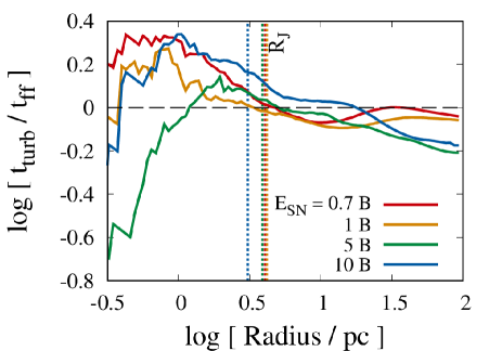
Fig. 5 shows the radial distribution of density, , , and of the gas particles as a function of distance from the density maximum of the enriched clouds. We also show half of the Jeans length (black dashed line) and the resolution limit defined as twice the smoothing length (red dotted line). The carbon and iron abundances show large deviations at distances pc because of the non-uniform metal mixing in the voids. Toward the higher density region at distances pc, the metal abundances converge. In Fig. 6 we compare the timescale for metal mixing due to turbulence, , with the free-fall timescale, , where and are the velocity dispersion and mean density within a radius , respectively. Within pc the mixing timescale becomes longer than the collapsing timescale, which indicates that further metal mixing does not occur as pointed out by earlier studies (Smith et al., 2015; Ritter et al., 2015; Chiaki & Wise, 2019).
We measure the average abundance of each element within pc, regarding it as the characteristic abundance of the clouds. The red and black curves in Fig. 7 show the elemental abundance ratios for the stratified and uniform ejecta, respectively. The difference of these abundances is within dex for all elements for all progenitor models (bottom panels of Fig. 7). We can conclude that the stratified structures of the ejecta hardly affect on the elemental abundance ratio of the internally enriched clouds, which we will further analyze in Section 3.2.1 (i).
For E10, metals reach the neighboring halo, and external enrichment (EE) occurs (Fig. 8) as well as IE. The blue curve of Fig. 9 shows that only the outer layers of ejecta with mass coordinates reach the neighboring halo. Since these layers mainly contain lighter elements (bottom panel of Fig. 7), the relative abundances of lighter elements () are enhanced more than . This indicates that stars with the C-enhanced abundance () can form in externally enriched clouds from normal CCSNe.


| 4enrich. | 11[C/Fe] | ||||||||||
|---|---|---|---|---|---|---|---|---|---|---|---|
| [Myr] | [] | [pc] | [] | [pc] | |||||||
| 5.69 | 26.4 | IE | 102 | ||||||||
| 7.30 | 26.2 | IE | 105 | ||||||||
| 24.7 | 23.9 | IE | 158 | ||||||||
| 37.2 | 22.5 | IE | 212 | ||||||||
| EE | 282 |
Note — (1) Explosion energy. (2) Time of recollapse from SN explosion. (3) Redshift of recollapse. (4) Enrichment mode. (5–6) Virial mass and radius of the MH at the time of recollapse. (7–8) Mass and half of the Jeans length of the recollapsing cloud. (9–11) Average carbon and iron abundances and relative abundance ratio of the recollapsing cloud. (12) Difference of between the stratified and uniform ejecta.
3.2 Evolution of SN shells
3.2.1 Internal enrichment
(i) General behavior
In the case of IE, there is only a slight difference ( dex) in the elemental abundance ratio between the clouds enriched by the stratified and uniform ejecta. Fig. 9 shows the mass fraction of metals falling back into the MH as a function of initial mass mass coordinate of the ejecta. For all , is almost constant against . Therefore, the ratio between lighter and heavier elements does not significantly deviate from that for the uniform ejecta.
In this section, we interpret this property by reviewing the evolution of SN shells. First, in the Sedov-Taylor (ST) phase, the shell evolves adiabatically because the timescale of radiative cooling is longer than the elapsed time. Then the shell enters the pressure-driven snowplough (PDS) phase, in which the dense cooling shell is pushed by the pressure in a hot inner cavity. Because of the inertial force from the decelerating shell to the ISM, RT instabilities develops and induces the mixing of materials between the shell and ISM. After the internal cavity cools down through radiative cooling, the shell continues to expand with its momentum being conserved in the phase called momentum-conserving snowplough (MCS) phase (Ostriker & McKee, 1988). The shell eventually either dissolves into the ISM if the explosion energy is enough high or otherwise falls back into the MH (Ritter et al., 2012; Sluder et al., 2016; Smith et al., 2015; Chiaki & Wise, 2019)
Figs. 3 and 4 show that lighter and heavier elements are both concentrated and partly mixed in the dense cooling shells which have developed in the PDS phase. As depicted by the dots with darker colors, both lighter and heavier elements that eventually fall back into the MH are confined in the same region where the SN shell interacts with the dense cosmological filaments. Using the radius of the filaments and the radius of the SN shell , we can estimate the fall back fraction as the ratio of the solid angles (Ritter et al., 2015). From this, the abundances of C and Fe which fall back can be estimated as
| (3) | |||||
| (4) |
where is the molecular weight of an element M (, ) and is the solar abundance of Fe (Asplund et al., 2009). The mass is defined as the Jeans mass of the recollapsing clouds. From these equations, the abundance ratio
| (5) |
is the same as that for the uniform ejecta
| (6) |
because the factor is canceled out. Since the factor depends only on the geometry of the circumstellar medium, the fall back fraction of each elements is almost the same.
For E0.7 and E5, the shell radius in the direction of filaments is pc and 60 pc, and the radius of the dense part of the filaments is pc and pc, respectively. Then, the enrichment fraction is and . This is consistent with the average fall back fraction estimated from our simulations ( and ; dotted lines in Fig. 9). With the typical mass of recollapsing clouds (Table 2), the abundances can be estimated to be (, ) = (, ) and (, ) for E0.7 and E5, respectively. These estimates are also consistent with the simulation results.
(ii) Dependency of elemental abundance on
The difference of the abundance ratio of lighter to heavier elements between the stratified and uniform ejecta depends slightly on . The bottom panels of Fig. 7 show that the ratio is higher than that from the uniform ejecta for lower explosion energies B () while similar or smaller for higher B (). The shell evolution and elemental abundances in the enriched clouds mostly differ between the two cases with explosion energies B and B, hereafter called low and high , respectively. We compare these two cases in this section.
For low , the MCS phase begins at Myr after the SN explosion. In the MCS phase, the contact surface of the shell in the direction of filaments is decelerated from the pressure of infalling gas along the filaments with a radial velocity (Fig. 1). In comparison, the hot inner part of the shell containing the heavier elements circumvents the dense contact surface and continues to expand in the direction of voids. Therefore, the abundance of Fe falling back into the cloud is slightly lower than the simple estimation of Eq. (4). As a result, the abundance ratio of lighter to heavier elements from the stratified ejecta becomes slightly larger than that from the uniform ejecta (). This is the consistent result with the high-resolution simulation of Ritter et al. (2015) and Sluder et al. (2016).
For high , the shell reaches a larger distance ( pc) and propagates into the less dense region () than for low (Fig. 4). The pressure from the filaments on the contact surface is smaller and the outer part of the shell is decelerated less efficiently. The inner part of the shell moves radially without circumventing the contact surface. Therefore, the deviation of the abundance ratio between lighter and heavier elements falling back into the MH is smaller than with lower . For E10, the elemental abundance ratio in the recollapsing cloud is consistent with that from the uniform ejecta (). However, for E5, the iron abundances are enhanced by dex. A part of the innermost layers that is initially in the direction to the void moves to the contact surface between the shell and filament because of the turbulence driven by the energetic explosion. This region contains 40.6% of the total iron mass that eventually falls back into the central MH. This results in the enhancement of iron relative to the elemental abundance of the uniform ejecta (), suggesting that the hydrodynamics in the shell can induce a dex of variation in the elemental abundance ratio.
3.2.2 External enrichment
For the EE case, in general, although metals reach a neighboring halo, they are hardly mixed with the gas in the central star-forming core (Chen et al., 2017; Chiaki et al., 2018). If gas density in the halo already exceeds a threshold value , the metals only superficially enrich the envelope of the cloud due to the pressure gradient. The metals can penetrate into the cloud center only if the SN energy is sufficiently strong (Chen et al., 2017) or if the halo merges with other halos (Chiaki et al., 2018). For E10, metals reach a neighboring halo initially at a distance pc from the central MH. The halo merges with two other halos (cyan circles in Fig. 1) at Myr after the SN explosion and then EE occurs. At Myr, the merged cloud becomes closer to the central MH with pc (Fig. 8). The radius of the region with densities above , which can trap metals, is pc (Fig. 5).
Only the outer layers of the ejecta with initial mass coordinates reach the neighboring halo. The fraction of the materials incorporated into the cloud is at (the blue curve in Fig. 9). This fraction can be explained with the simple estimation used in Section 3.2.1 as . With the mass of the enriched cloud , we can estimate the C abundance of the enriched cloud to be from Eq. (3), consistent with the simulation result (Table 2). The abundance is much smaller than those in the case with IE by dex because the metals are diluted by the larger mass of pristine gas by two orders of magnitude than the typical cloud mass (). The cloud mass is much larger because the halo hosting the cloud grows through a set of mergers before EE occurs.

4 Discussion
4.1 Prediction of observations
If low-mass stars () form in the enriched clouds, they can survive for the Hubble time (Smith et al., 2015; Chiaki & Wise, 2019). Then, if some of the stars are accreted onto our Milky Way halo or local dwarf galaxies through cosmic structure formation, they can be observed as EMP stars (Frebel & Norris, 2015, and references therein). The colored symbols in Fig. 10 show the distribution of the stars on the - plane. The closed and open symbols depict the abundances of stars forming in the internally and externally enriched clouds (hereafter called IE-stars and EE-stars), respectively. The small and large symbols depict the abundances for the uniform and stratified ejecta, respectively. Interestingly, the Fe abundances are shifted while C abundances hardly change. The mass of the outer layers is larger than that of the inner layers, where the fall back fraction fluctuates, and the mass-weighted average fraction is closer to the fraction in the outer layers (Fig. 9).
For comparison, we also plot the C and Fe abundances of observed C-normal and C-enhanced stars with blue and red dots, respectively (taken from the SAGA database; Suda et al., 2008). The stars with below and above (dashed line) are defined as C-normal stars and CEMP stars, respectively (Aoki et al., 2007). C-normal stars are distributed around the line (dot-dashed line). CEMP stars with are classified into two sub-groups according to their distributions (Yoon et al., 2016). Group III stars are distributed around the horizontal line with a constant while Group II stars are distributed along the line with a constant and just above the region where C-normal stars are distributed. The show the large star-to-star scatter of dex with a fixed metallicity for all groups. This can be considered to reflect the variation of mass and explosion energy of few progenitor stars in the early stage of galactic chemical evolution (Ryan et al., 1996; Cayrel et al., 2004).
From our simulations, the IE-stars are distributed around the line (dot-dashed line) with dex deviation. This is consistent with the distribution of observed C-normal and Group II stars. For B (green circle and blue square), the IE-stars have low values (bottom right in Fig. 10) because for a uniform ejecta ( and ) is smaller than the solar abundance ratio, and is unchanged or depleted by the effect of the stratified ejecta. For B (red diamond and orange triangle), is larger (0.48 and 0.31) for the uniform ejecta and further enhanced for the stratified ejecta (see Section 3.2.1 ii). The stars are distributed around the critical line for CEMP stars (dashed line). For B, the stars would be classified as CEMP stars (red diamond). In this work, we fix the progenitor mass to , but the range of explosion energies (0.7–10 B) can explain the distribution of observed C-normal and CEMP Group II stars with a scatter of dex.
For EE-stars, both and are smaller than the ones of IE-stars by two orders of magnitude because metals are mixed with a large mass of pristine gas during a merger of three host halo progenitors which induces EE (Section 3.2.2). As a result, and of the EE-stars exist in the low metallicity region where stars have not been observed (grey shaded region in Fig. 10). We can consider several reasons why these EE-stars with extremely small metallicities have not been observed. First, because the metallicity for IE is larger than that for EE, the C-enhanced abundance pattern resulting from EE may be washed out by the IE of the neighboring cloud itself. Halos only externally enriched may be so rare that EE-stars have not so far been observed among the current samples of EMP stars (Hartwig et al., 2018). Second, clouds with insufficient metal content () should contain a negligible amount of dust grains, which is the main coolant that can induce cloud fragmentation. Chiaki et al. (2017) estimate the elemental abundances below which dust cooling works inefficiently as (purple curve in Fig. 10). The EE-stars are plotted below this curve, where clouds can collapse stably against fragmentation, and a single massive star () is likely to form. Such massive stars can not be observed because they will not survive for 13.6 Gyr between the recollapsing redshift and the present day.
4.2 Caveats
In this work, we perform numerical simulations of the transition from Pop III stars to Pop II stars, considering the non-uniform structure of SN ejecta with realistic nucleosynthesis models. Because of computational limits, there are several caveats in the simulations.
4.2.1 Resolution of simulations
In the simulations, the SPH particle mass is , and the number of neighboring particles is . The number of particles that resolve half of the Jeans length of the collapsing clouds with a density and temperature K is
| (7) |
where is the smoothing length. This resolution is lower than adaptive mesh refinement (AMR) simulations of chemical enrichment (Ritter et al., 2012; Smith et al., 2015; Chiaki & Wise, 2019).
The Strömgren radius is not properly resolved just before the SN explosion (Section 2.2). In an AMR simulation of Ritter et al. (2012), the region within a few pc is fully ionized by a Pop III star with a mass , and the density of the H ii region decreases down to a few . To resolve the H ii region, we could use refinement techniques, such as particle splitting. Also, de-refinement of the particles are required just before the SN explosion to follow the expansion of SN shells for the reason stated below. The refinement and de-refinement procedures would induce numerical errors (Chiaki & Yoshida, 2015). Eitherway, at the time of the SN, we inject metals and thermal energy in a sphere with a radius pc comparable to the expected radius of the H ii region. Therefore, in this work, we do not refine or de-refine particles for the formation of H ii region.
| 2enrich. | 6[C/Fe] | [C/Fe] | ||||
|---|---|---|---|---|---|---|
| [pc] | ||||||
| IE | ||||||
| IE | ||||||
| IE | ||||||
| IE | ||||||
| EE |
Note — (1) Explosion energy. (2) Enrichment mode. (3) Half of the Jeans radius. (4–6) Average carbon and iron abundances and relative abundance ratio within . (12) Difference of between the stratified and uniform ejecta.
We cannot use particle splitting after a SN explosion to resolve a cooling shell and a recollapsing cloud because particles in the dense regions such as ejecta and shocked shell would be refined and blown away by SN blastwaves to the outer region filled with coarse particles. In the interacting regions between particles with different masses, spurious surface tension would affect the estimation of hydrodynamic force (Saitoh & Makino, 2013). Although we barely resolve the Jeans length of the recollapsing clouds, the elemental abundance ratio for E1 is consistent with the results of higher-resolution simulations of Ritter et al. (2015) and Sluder et al. (2016) for the same . Also, the low-resolution simulations enable us to investigate the metal enrichment for the wide range of explosion energies – B.
4.2.2 Abundance in inner region of enriched clouds
Fig. 5 shows that the elemental abundance still has dex deviation at half of the Jeans length from the collapse center (black dashed line). Further, systematically decreases or increases toward the center within for E0.7 and E5, respectively. In the succeeding run-away collapse phase, the mass of the cloud core decreases as the maximum density increases (Larson, 1969). Therefore, the stars that finally form might have the elemental abundance of the innermost region of the cloud. We estimate the average abundance of the cloud within (red dotted lines). As Table 3 shows, the difference of abundance ratio becomes larger ( dex for IE) than that within (Table 2). The region within is resolved only two smoothing lengths of SPH particles (Eq. 7), and thus we can hardly conclude that the abundances would reflect this value. Simulations with higher resolution are thus required to determine the elemental abundances of stars that would eventually form. We will perform AMR simulations to clarify the metal mixing in higher density regions in forthcoming papers.
4.2.3 Mass and multiplicity of Pop III
In this paper, we fix the Pop III stellar mass to . This assumption is justified from some numerical simulations showing that the peak of the Pop III mass distribution is around (Susa et al., 2014; Hirano et al., 2014, 2015). Also, Ishigaki et al. (2018) find that elemental abundances of most EMP stars are best fit with a Pop III hypernova model with a progenitor mass . However, these studies also suggest a range of stellar mass (–), which can yield a variety of elemental abundance patterns. We need to study metal enrichment with different Pop III stellar masses to understand the full abundance distribution of EMP stars (Fig. 10). Further, we assume that the MH hosts only a single Pop III star. Recent numerical simulations show that multiple Pop III stars form through the fragmentation of the accretion disk (Turk et al., 2009; Clark et al., 2011; Greif et al., 2012; Susa et al., 2014; Hirano & Bromm, 2017). The elemental abundance of enriched clouds will be the superposition of elemental abundances of multiple progenitor stars (Feng & Krumholz, 2014; Ritter et al., 2015).
We consider a single MH with a mass . Although this is the typical mass of Pop III hosting MHs (Fig. 12 of Chiaki et al., 2018), MHs have a wide mass range from to . For low-mass MHs (), a massive Pop III star () can create the H ii region with radii larger than the virial radius, and the SN shell can expand without losing its thermal and kinetic energy. Metals can reach neighboring MHs, and EE mainly occurs. On the other hand, for Pop III stars with masses and explosion energies B, IE is the main enrichment channel. For high-mass MHs (), IE mainly occurs even for massive Pop III stars and energetic SNe (Chiaki et al., 2018).
We do not include the effect of streaming velocity, which in general occurs due to the different evolution of dark matter and baryon density fluctuations before the recombination (Tseliakhovich & Hirata, 2010). This results in the delayed star formation caused by the offset of dense gas clumps from dark matter potential wells (Chiou et al., 2018, 2019; Druschke et al., 2019). Star formation occurs in more massive halos () than zero-streaming velocity cases, where EE hardly occur even for high (Chiaki et al., 2018). Previous studies also predict that clouds with surpersonic turbulence may fragment to massive Pop III star clusters (Hirano et al., 2018), indicating that the mixing of metals from multiple sources may be more significant.
4.2.4 Stars with peculiar elemental abundance
We use SN models that reproduce the elemental abundances of C-normal EMP stars with . However, % of EMP stars with metallicities show C-enhanced abundance pattern (Yoon et al., 2018; Norris & Yong, 2019). Several scenarios have been proposed to explain the CEMP star formation. One is the intrinsic enrichment scenario in which parent clouds of the stars are enriched by C-enhanced interstellar gas. The source of C-rich gas is considered to be SNe with a large fallback of Fe-rich innermost layers into the central remnant and ejection of C-rich outer layers into the ISM (faint SNe; Umeda & Nomoto, 2003). The other is the extrinsic enrichment scenario in which C-rich gas accretes onto the surface of stars from their binary companion in the asymptotic giant branch (AGB) phase (Suda et al., 2004; Komiya et al., 2020).
We can simply apply this work to the faint SN model by assigning the corresponding radial distribution of elemental mass fraction to the metal tracer particles. As Fig. 9 shows, the fraction of metals incorporated into the enriched ejecta is almost constant in the outer layers but deviated from this constant value in the innermost layers. Since elements lighter than Fe are dominant in the innermost region of faint SN ejecta, the slight deviation of their abundances might be seen for faint SNe.
Stellar rotation can also modify the elemental abundance in the final phase of stellar evolution. The elemental abundance of materials blown away from the ensuing SN explosion shows C, N, and s-process element enhancement (Meynet et al., 2006; Choplin et al., 2017). In addition, the rotating stars are considered to explode as jet-like SNe. This model is introduced to explain Si-deficient of the star HE and Zn-enhancement of the star HE (Tominaga, 2009; Ezzeddine et al., 2019). The elemental abundance of clouds enriched from this type of SNe should strongly depend on the direction of the jets against the three-dimensional structure of the intergalactic medium. We will see the enrichment process of jet-like SNe in forthcoming papers.
5 Conclusion
We perform numerical simulations focusing on the metal enrichment from Pop III SNe, considering a stratified structure of ejecta. Here we consider normal core-collapse supernova (CCSN) models with . We find that SN shells fall back into the central minihalo in all models. The abundance ratio in the recollapsing clouds deviates from that from the uniform ejecta by at most dex for any element M. Overall, the fraction of metals falling back into the recollapsing clouds is almost constant regardless of the initial mass coordinate of the ejecta. The slight deviation from the average abundance of the ejecta is mainly from the turbulent motion of the hot innermost layers. The metallicity range of these clouds is and resulting C to Fe abundance ratio is . If the stars directly inherit the elemental abundance of their host clouds, the abundances of the stars are consistent with those of the observed C-normal and Group II CEMP stars.
In addition, for the largest explosion energy (10 B), a neighboring halo is also enriched. Only the outer layers rich with Ca or lighter elements reach the halo, where the abundance ratio of C to Fe is . This means that C-enhanced metal-poor (CEMP) stars can form from the CCSN with the average abundances ratio . However, the metallicity of this cloud is smaller than in the IE cases by two orders of magnitude because the halo contains a large mass of pristine gas () before it is enriched. In the low-metallicity region, no low-mass stars have so far been observed. With a statistic analysis, the hypothesis that these stars escape the detection is ruled out at a 99.9% confidence level with samples of EMP stars observed so far (Magg et al., 2019). An explanation of the non-detection is that such a low-metallicity cloud will collapse stably without fragmentation because of a lack of cooling from dust grains. Massive stars are likely to form and not be observed due to their short lifetime compared to the Hubble time (Chiaki et al., 2017).
In this paper, we have studied the metal enrichment from normal CCSNe with a fixed progenitor mass. Nowadays stars have been observed with large survey campaigns, and EMP stars have been identified with follow-up spectroscopic measurements. These observations have revealed that there are various classifications of EMP stars with an enhancement or depletion of specific elements. We will extend our numerical methods to the other types of SN models such as rotating stars, faint SN models and jet-like SN models (Section 4.2.4) to construct the comprehensive formation models of statistical samples of EMP stars. These studies will uncover the general process of chemical enrichment in the ISM and the origins of elements that compose the Universe.
ACKNOWLEDGMENTS
We thank John H. Wise for fruitful discussions and comments. GC is supported by Overseas Research Fellowships of the Japan Society for the Promotion of Science (JSPS) for Young Scientists. The numerical simulations and analyses in this work are carried out on XC40 in Yukawa Institute of Theoretical Physics (Kyoto University), Comet in SDSC, Stampede2 in TACC on NSF’s XSEDE allocation AST-120046, and PACE/HIVE clusters in the Georgia Institute of Technology. The figures in this paper are constructed with the plotting library gnuplot and matplotlib (Hunter, 2007).
Data availability
The data underlying this article will be shared on reasonable request to the authors.
References
- Abel et al. (2002) Abel, T., Bryan, G. L., & Norman, M. L. 2002, Science, 295, 93
- Aoki et al. (2007) Aoki, W., Beers, T. C., Christlieb, N., et al. 2007, ApJ, 655, 492
- Asplund (2005) Asplund M., 2005, ARA&A, 43, 481
- Asplund et al. (2009) Asplund, M., Grevesse, N., Sauval, A. J., & Scott, P. 2009, ARA&A, 47, 481
- Beers et al. (1985) Beers, T. C., Preston, G. W., & Shectman, S. A. 1985, AJ, 90, 2089
- Beers et al. (1992) Beers, T. C., Preston, G. W., & Shectman, S. A. 1992, AJ, 103, 1987
- Beers & Christlieb (2005) Beers, T. C., & Christlieb, N. 2005, ARA&A, 43, 531
- Belczynski et al. (2010) Belczynski K., Bulik T., Fryer C. L., Ruiter A., Valsecchi F., Vink J. S., Hurley J. R., 2010, ApJ, 714, 1217
- Bromm et al. (1999) Bromm, V., Coppi, P. S., & Larson, R. B. 1999, ApJ, 527, L5
- Caffau et al. (2011b) Caffau, E., Bonifacio, P., François, P., et al. 2011, Nature, 477, 67
- Cayrel et al. (2004) Cayrel, R., Depagne, E., Spite, M., et al. 2004, A&A, 416, 1117
- Clark et al. (2011) Clark, P. C., Glover, S. C. O., Smith, R. J., et al. 2011, Science, 331, 1040
- Chen et al. (2017) Chen, K.-J., Whalen, D. J., Wollenberg, K. M. J., Glover, S. C. O., & Klessen, R. S. 2017, ApJ, 844, 111
- Chiaki & Yoshida (2015) Chiaki, G., & Yoshida, N. 2015, MNRAS, 451, 3955
- Chiaki et al. (2017) Chiaki, G., Tominaga, N., & Nozawa, T. 2017, MNRAS, 472, L115
- Chiaki et al. (2018) Chiaki, G., Susa, H., & Hirano, S. 2018, MNRAS, 475, 4378
- Chiaki & Wise (2019) Chiaki, G., & Wise, J. H. 2019, MNRAS, 482, 3933
- Chiou et al. (2018) Chiou Y. S., Naoz S., Marinacci F., Vogelsberger M., 2018, MNRAS, 481, 3108
- Chiou et al. (2019) Chiou Y. S., Naoz S., Burkhart B., Marinacci F., Vogelsberger M., 2019, ApJL, 878, L23
- Choplin et al. (2017) Choplin A., Ekström S., Meynet G., Maeder A., Georgy C., Hirschi R., 2017, A&A, 605, A63
- Christlieb (2003) Christlieb, N. 2003, in Reviews in Modern Astronomy, Vol. 16, Reviews in Modern Astronomy, ed. R. E. Schielicke, 191
- Cui et al. (2012) Cui, X.-Q., Zhao, Y.-H., Chu, Y.-Q., et al. 2012, Research in Astronomy and Astrophysics, 12, 1197
- Deng et al. (2012) Deng, L.-C., Newberg, H. J., Liu, C., et al. 2012, Research in Astronomy and Astrophysics, 12, 735
- Dotani et al. (1987) Dotani T., et al., 1987, Natur, 330, 230
- Douvion et al. (2001) Douvion T., Lagage P. O., Cesarsky C. J., Dwek E., 2001, A&A, 373, 281
- Druschke et al. (2019) Druschke M., Schauer A. T. P., Glover S. C. O., Klessen R. S., 2019, arXiv, arXiv:1906.09845
- Ezzeddine et al. (2019) Ezzeddine R., et al., 2019, ApJ, 876, 97
- Feng & Krumholz (2014) Feng Y., Krumholz M. R., 2014, Natur, 513, 523
- Frebel & Norris (2015) Frebel A., Norris J. E., 2015, ARA&A, 53, 631
- Gratton et al. (2000) Gratton R. G., Sneden C., Carretta E., Bragaglia A., 2000, A&A, 354, 169
- Greif et al. (2012) Greif, T. H., Bromm, V., Clark, P. C., et al. 2012, MNRAS, 424, 399
- Hartwig et al. (2018) Hartwig, T., Yoshida, N., Magg, M., et al. 2018, MNRAS, 478, 1795
- Hahn & Abel (2011) Hahn, O., & Abel, T. 2011, MNRAS, 415, 2101
- Hirano et al. (2014) Hirano, S., Hosokawa, T., Yoshida, N., et al. 2014, ApJ, 781, 60
- Hirano et al. (2015) Hirano, S., Hosokawa, T., Yoshida, N., Omukai, K., & Yorke, H. W. 2015, MNRAS, 448, 568
- Hirano & Bromm (2017) Hirano, S., & Bromm, V. 2017, MNRAS, 470, 898
- Hirano et al. (2018) Hirano S., Yoshida N., Sakurai Y., Fujii M. S., 2018, ApJ, 855, 17
- Hopkins (2013) Hopkins, P. F. 2013, MNRAS, 428, 2840
- Hunter (2007) Hunter J. D., 2007, CSE, 9, 90
- Ishigaki et al. (2018) Ishigaki, M. N., Tominaga, N., Kobayashi, C., & Nomoto, K. 2018, arXiv:1801.07763
- Iwamoto et al. (1998) Iwamoto K., et al., 1998, Natur, 395, 672
- Jappsen et al. (2007) Jappsen, A.-K., Glover, S. C. O., Klessen, R. S., & Mac Low, M.-M. 2007, ApJ, 660, 1332
- Joggerst, Almgren & Woosley (2010) Joggerst C. C., Almgren A., Woosley S. E., 2010, ApJ, 723, 353
- Keller et al. (2014) Keller, S. C., Bessell, M. S., Frebel, A., et al. 2014, Nature, 506, 463
- Kitayama et al. (2004) Kitayama, T., Yoshida, N., Susa, H., & Umemura, M. 2004, ApJ, 613, 631
- Kitayama & Yoshida (2005) Kitayama, T., & Yoshida, N. 2005, ApJ, 630, 675
- Komiya et al. (2020) Komiya Y., Suda T., Yamada S., Fujimoto M. Y., 2020, ApJ, 890, 66
- Larson (1969) Larson, R. B. 1969, MNRAS, 145, 271
- Magg et al. (2017) Magg, M., Hartwig, T., Agarwal, B., et al. 2017, arXiv:1706.07054
- Magg et al. (2019) Magg M., Klessen R. S., Glover S. C. O., Li H., 2019, MNRAS, 487, 486
- McKee & Ostriker (1977) McKee C. F., Ostriker J. P., 1977, ApJ, 218, 148
- Meynet et al. (2006) Meynet G., Ekström S., Maeder A., 2006, A&A, 447, 623
- Norris & Yong (2019) Norris J. E., Yong D., 2019, ApJ, 879, 37
- Omukai (2000) Omukai, K. 2000, ApJ, 534, 809
- Omukai et al. (2005) Omukai, K., Tsuribe, T., Schneider, R., & Ferrara, A. 2005, ApJ, 626, 627
- Ostriker & McKee (1988) Ostriker J. P., McKee C. F., 1988, RvMP, 60, 1
- Planck Collaboration et al. (2016) Planck Collaboration, Ade, P. A. R., Aghanim, N., et al. 2016, A&A, 594, A13
- Placco et al. (2014) Placco V. M., Frebel A., Beers T. C., Stancliffe R. J., 2014, ApJ, 797, 21
- Ritter et al. (2012) Ritter, J. S., Safranek-Shrader, C., Gnat, O., Milosavljević, M., & Bromm, V. 2012, ApJ, 761, 56
- Ritter et al. (2015) Ritter, J. S., Sluder, A., Safranek-Shrader, C., Milosavljević, M., & Bromm, V. 2015, MNRAS, 451, 1190
- Ritter et al. (2016) Ritter, J. S., Safranek-Shrader, C., Milosavljević, M., & Bromm, V. 2016, MNRAS, 463, 3354
- Ryan et al. (1996) Ryan, S. G., Norris, J. E., & Beers, T. C. 1996, ApJ, 471, 254
- Saitoh & Makino (2009) Saitoh, T. R., & Makino, J. 2009, ApJ, 697, L99
- Saitoh & Makino (2013) Saitoh, T. R., & Makino, J. 2013, ApJ, 768, 44
- Schaerer (2002) Schaerer, D. 2002, A&A, 382, 28
- Schneider et al. (2003) Schneider, R., Ferrara, A., Salvaterra, R., Omukai, K., & Bromm, V. 2003, Nature, 422, 869
- Sluder et al. (2016) Sluder, A., Ritter, J. S., Safranek-Shrader, C., Milosavljević, M., & Bromm, V. 2016, MNRAS, 456, 1410
- Smith et al. (2008) Smith, B., Sigurdsson, S., & Abel, T. 2008, MNRAS, 385, 1443
- Smith et al. (2015) Smith, B. D., Wise, J. H., O’Shea, B. W., Norman, M. L., & Khochfar, S. 2015, MNRAS, 452, 2822
- Springel (2005) Springel, V. 2005, MNRAS, 364, 1105
- Stacy & Bromm (2014) Stacy, A., & Bromm, V. 2014, ApJ, 785, 73
- Suda et al. (2004) Suda, T., Aikawa, M., Machida, M. N., Fujimoto, M. Y., & Iben, I., Jr. 2004, ApJ, 611, 476
- Suda et al. (2008) Suda, T., Katsuta, Y., Yamada, S., et al. 2008, PASJ, 60, 1159
- Susa (2006) Susa, H. 2006, PASJ, 58, 445
- Susa et al. (2014) Susa, H., Hasegawa, K., & Tominaga, N. 2014, ApJ, 792, 32
- Tanaka et al. (2017) Tanaka, S. J., Chiaki, G., Tominaga, N., & Susa, H. 2017, ApJ, 844, 137
- Tominaga (2009) Tominaga N., 2009, ApJ, 690, 526
- Tominaga et al. (2014) Tominaga, N., Iwamoto, N., & Nomoto, K. 2014, ApJ, 785, 98
- Truelove et al. (1997) Truelove, J. K., Klein, R. I., McKee, C. F., et al. 1997, ApJ, 489, L179
- Tseliakhovich & Hirata (2010) Tseliakhovich D., Hirata C., 2010, PhRvD, 82, 083520
- Turk et al. (2009) Turk, M. J., Abel, T., & O’Shea, B. 2009, Science, 325, 601
- Umeda & Nomoto (2003) Umeda, H., & Nomoto, K. 2003, Nature, 422, 871
- Wadsley, Keller & Quinn (2017) Wadsley J. W., Keller B. W., Quinn T. R., 2017, MNRAS, 471, 2357
- Yanny et al. (2009) Yanny, B., Rockosi, C., Newberg, H. J., et al. 2009, AJ, 137, 4377-4399
- Yoon et al. (2016) Yoon, J., Beers, T. C., Placco, V. M., et al. 2016, ApJ, 833, 20
- Yoon et al. (2018) Yoon, J., Beers, T. C., Dietz, S., et al. 2018, arXiv:1806.04738