Diversity-Promoting Ensemble for Medical Image Segmentation

Mariana-Iuliana Georgescu University of BucharestRomania , Radu Tudor Ionescu University of BucharestRomania [email protected] and Andreea-Iuliana Miron “Carol Davila” University of Medicine and Pharmacy, Colţea HospitalRomania

(2023)

Abstract.

Medical image segmentation is an actively studied task in medical imaging, where the precision of the annotations is of utter importance towards accurate diagnosis and treatment. In recent years, the task has been approached with various deep learning systems, among the most popular models being U-Net. In this work, we propose a novel strategy to generate ensembles of different architectures for medical image segmentation, by leveraging the diversity (decorrelation) of the models forming the ensemble. More specifically, we utilize the Dice score among model pairs to estimate the correlation between the outputs of the two models forming each pair. To promote diversity, we select models with low Dice scores among each other. We carry out gastro-intestinal tract image segmentation experiments to compare our diversity-promoting ensemble (DiPE) with another strategy to create ensembles based on selecting the top scoring U-Net models. Our empirical results show that DiPE surpasses both individual models as well as the ensemble creation strategy based on selecting the top scoring models.

medical imaging; medical image segmentation; model ensemble; neural network ensemble; deep learning; neural networks; voting-based ensemble; plurality voting.

^†^†journalyear: 2023^†^†copyright: acmlicensed^†^†conference: The 37th ACM/SIGAPP Symposium on Applied Computing; March 27-April 2, 2023; Tallinn, Estonia^†^†booktitle: The 37th ACM/SIGAPP Symposium on Applied Computing (SAC ’23), March 27-April 2, 2023, Tallinn, Estonia^†^†price: 15.00^†^†doi: 10.1145/3555776.3577682^†^†isbn: 978-1-4503-9517-5/23/03^†^†article: 12927.99^†^†ccs: Computing methodologies Supervised learning^†^†ccs: Computing methodologies Image processing^†^†ccs: Computing methodologies Image segmentation^†^†ccs: Applied computing Health informatics

1. Introduction

Physicians extensively use medical imaging techniques, e.g. Computed Tomography (CT), Magnetic Resonance Imaging (MRI) and Optical Coherence Tomography (OCT) (Verga et al., 2014), as one of the least invasive investigation alternatives to diagnose lesions inside the human body. Segmenting (delimiting) regions of interest, such as organs or tumors, is often required for precise diagnosis and treatment. For example, a precise segmentation of a malignant tumor can lead to an accurate calibration of the radiation dosage in radiotherapy (Jin et al., 2021; Wang et al., 2018; Men et al., 2018; Seo et al., 2020). In recent years, the medical image segmentation task has been approached with various deep learning systems, ranging from convolutional neural networks (CNNs) (Ronneberger et al., 2015; Seo et al., 2020; Alom et al., 2019) to transformers (Chen et al., 2021; Gao et al., 2021; Hatamizadeh et al., 2022). Among these, U-Net (Ronneberger et al., 2015) remains one of the most popular methods. Although U-Net was introduced in 2015, it consistently received updates (Siddique et al., 2021; Zhou et al., 2018; Alom et al., 2019; Oktay et al., 2018), keeping its performance at a competitive level. However, using a single neural network to perform segmentation is not always the best solution. Indeed, constructing ensembles of multiple neural networks is an extensively validated method (Lyksborg et al., 2015; Baldeon Calisto and Lai-Yuen, 2020; Zhao et al., 2019; Ganaie et al., 2022) to boost accuracy.

Since the precision of the medical image segmentation output is of utter importance towards accurate diagnosis and treatment, we focus on combining multiple U-Net architectures to address the task. We conjecture that decorrelated models lead to a superior ensemble, since decorrelated models can better complement each other’s decisions. To this end, we propose a novel strategy to construct ensembles of different models for medical image segmentation by promoting the diversity (decorrelation) of the models comprising the ensemble, while also giving equal importance to accuracy. To measure the correlation among two models, we compute the Dice score between the outputs of the respective models. We then construct the ensemble in a bottom-up fashion, starting from the best model and gradually adding the least correlated models with those already included, one by one. At the same time, our ensemble creation strategy assigns equal importance to the performance level of the model to be added at each step. Since we select models with lower Dice scores at each step, our strategy promotes the diversity among the models comprising the ensemble, hence bearing the name Diversity-Promoting Ensemble (DiPE).

We conduct image segmentation experiments on the gastro-intestinal tract data set provided by the UW-Madison Carbone Cancer Center (Lee et al., 2022). We evaluate nine individual U-Net models based on three different backbones (ResNet-34 (He et al., 2016), EfficientNet-B0 (Tan and Le, 2019), EfficientNet-B1 (Tan and Le, 2019)) with or without multi-head convolutional attention (Georgescu et al., 2023). Along with the individual models, we evaluate two strategies to create voting-based ensembles, namely $(i)$ a baseline (conventional) strategy selecting the top scoring models and $(ii)$ our strategy promoting diversity among the selected models. The empirical results indicate that our strategy, DiPE, outperforms both individual models, as well as the baseline ensemble.

In summary, our contribution is twofold:

•

We introduce a diversity-promoting strategy to create an ensemble of medical image segmentation models that are low correlated among each other, by leveraging the Dice score between the outputs of various models.
•

We provide empirical evidence showing that our diversity-promoting ensemble leads to superior performance levels compared with individual models and the conventional strategy selecting the top scoring models.

2. Related Work

Medical image segmentation can be divided into two tasks, with respect to the input image. Indeed, there are works that tackle the segmentation task on 2D images (Ronneberger et al., 2015; Luo et al., 2021; Zhao et al., 2022; Wang et al., 2018), while others rely on 3D images (Chen et al., 2018; Kamnitsas et al., 2017; Gibson et al., 2018; Luo et al., 2021; Zhao et al., 2022; Chen et al., 2022a; Wolz et al., 2013; Lyksborg et al., 2015; Baldeon Calisto and Lai-Yuen, 2020; Seo et al., 2020; Jin et al., 2021). The works using 2D images as input naturally produce 2D slices as output, while the works using entire 3D volumes as input produce 3D volumes as output.

Perhaps the most popular architecture for 2D segmentation is U-Net (Ronneberger et al., 2015). U-Net is a fully convolutional (conv) network designed for medical image segmentation. The architecture follows a “U” shape and is composed of a contracting and an expansive path. Each step of the expansive path is composed of an upsampling operation, a convolution layer which halves the number of feature maps, and a concatenation with the corresponding cropped feature maps from the contracting path. Seo et al. (Seo et al., 2020) proposed the mU-Net model, a modified version of the U-Net architecture. mU-Net (Seo et al., 2020) adds a residual path to the deconvolution operations, and an additional convolutional layer to the skip connections in order to extract high-level global features of small objects.

Chen et al. (Chen et al., 2018) proposed the voxel-wise residual network (VoxResNet), a 3D CNN formed of 25 layers with residual connections. Multimodal and multi-level contextual information is introduced into the VoxResNet model. The multimodal information is added by concatenating multimodal data before giving it as input to the model. To improve the 3D segmentation performance of brain lesions, Kamnitsas et al. (Kamnitsas et al., 2017) employed a 3D CNN comprising 11 layers with parallel convolutional pathways for multi-scale processing. Rather than modifying the layers of their architecture, Zhao et al. (Zhao et al., 2022) inserted a lesion-related spatial attention mechanism into the network.

In order to help physicians obtain better segmentation results, Luo et al. (Luo et al., 2021) proposed interactive segmentation to further improve the performance of CNN models, even to unseen objects.

Closer to our study, the work of Gibson et al. (Gibson et al., 2018) shares the same target task, being focused on multi-organ abdominal segmentation. Gibson et al. (Gibson et al., 2018) presented a registration-free approach based on Dense V-Networks for multi-organ abdominal segmentation of 3D images. They also proposed a batch-wise spatial dropout to lower the memory usage and processing time of dropout.

Different from the aforementioned works, which are trained in a fully-supervised learning setting, there are several works (Zhou et al., 2019; Chen et al., 2022b) proposing weakly-supervised learning frameworks. Zhou et al. (Zhou et al., 2019) found that data sets having only one organ annotated as the positive class, leaving the other organs as part of the background, attain misleading results in multi-organ segmentation, since the background class contains many organs. In order to alleviate this problem, Zhou et al. (Zhou et al., 2019) proposed a prior-aware neural network, incorporating anatomical priors on abdominal organ sizes into the training objective.

Similar to our approach proposing an ensemble of multiple networks to improve the segmentation results, Lyksborg (Lyksborg et al., 2015) proposed to use a model for each of the axial, sagittal and coronal planes, fusing the corresponding segmentations into a single 3D segmentation. Baldeon et al. (Baldeon Calisto and Lai-Yuen, 2020) proposed AdaEn-Net, an ensemble of networks that boosts the segmentation performance. AdaEn-Net (Baldeon Calisto and Lai-Yuen, 2020) firstly employs an ensemble of 2D and 3D models to predict the output segmentation. Then, it trains the 2D-3D ensemble on $k$ -folds, obtaining $k$ models. The final segmentation mask is the average of the $k$ models forming the final ensemble.

Different from previous works, such as (Lyksborg et al., 2015; Baldeon Calisto and Lai-Yuen, 2020), which directly combined models into ensembles without taking into account their output correlation, we propose a novel ensemble creation algorithm which promotes the diversity among the models comprising the ensemble.

3. Method

3.1. Neural Architectures

To address our medical image segmentation task, we employ the well known U-Net architecture (Ronneberger et al., 2015). The U-Net architecture is a fully convolutional network that belongs to the family of encoder-decoder neural networks. In the encoding part, the spatial information is downsampled through convolution and pooling operations. In the decoding part, the spatial information is upsampled back to the original size via convolution transpose. High-resolution features from the encoder are passed through skip connections and concatenated to the corresponding features from the decoder, thus infusing high-resolution information into the decoder. The introduction of skip connections gives the network its “U” shape. We further present our changes to the U-Net model, leading to a total of nine distinct model variants forming the basis of our ensemble.

Refer to caption — Figure 1. Correlation matrix based on paired Dice coefficients between the individual U-Net models included in our study.

3.1.1. Backbone Variations

To build an ensemble of a diverse set of models, we first introduce variations in terms of the backbone architecture. Therefore, we try the following three encoder architectures: ResNet-34 (He et al., 2016), EfficientNet-B0 (Tan and Le, 2019), and EfficientNet-B1 (Tan and Le, 2019). We choose ResNet-34 due to its fairly good trade-off between running time and accuracy level. The reason behind adding EfficientNet-B0 and EfficientNet-B1 into our study is the superior performance levels of these models compared to ResNet-34.

The residual network (ResNet) architecture was proposed by He et al. (He et al., 2016). ResNet models are composed of residual blocks. A residual block consists of a few stacked conv layers and a skip connection from the first layer to the last layer of the block. Skip connections allow the training of very deep neural networks, alleviating the vanishing gradient problem. He et al. (He et al., 2016) proposed five ResNet variants of different depth, namely ResNet-18, ResNet-34, ResNet-50, ResNet-101 and ResNet-152. Among these, we select ResNet-34 to serve as backbone for some of our U-Net models.

The EfficientNet architecture was introduced by Tan et al. (Tan and Le, 2019) to efficiently scale convolutional neural networks. Tan et al. (Tan and Le, 2019) demonstrated that, in order to obtain better performance under a certain computational budget, all three components of the network, namely the depth, the width and the resolution, should be uniformly scaled. Based on this finding, the EfficientNet family of models (from B1 to B7) was created starting from the EfficientNet-B0 architecture and scaling the depth, width and resolution of each network version by a certain factor. EfficientNets generally obtain better performance than the previous state-of-the-art convolutional networks under the same computational resources.

We employ the same decoder architecture, regardless of the encoder type. More specifically, the decoder is formed of five successive convolutional blocks with the following number of filters: $512$ , $256$ , $128$ , $64$ and $64$ . Inside the decoder, we use nearest neighbor interpolation as the upsampling operation.

3.1.2. Integrating Attention

In order to further increase the variability of the studied models, we add a newly introduced multi-head convolutional attention (MHCA) (Georgescu et al., 2023) mechanism. MHCA performs both channel and spatial attention by applying multiple convolutional attention heads. Each convolutional head has a distinct receptive field size corresponding to a particular reduction rate for the spatial attention. At the same time, the number of filters is used to control the channel reduction rate. The MHCA (Georgescu et al., 2023) block can be introduced at any layer of any neural architecture.

We underline that the MHCA (Georgescu et al., 2023) block was originally introduced for medical image super-resolution. We opt for introducing the MHCA module instead of other popular attention mechanisms, e.g. Squeeze-and-Excitation (Hu et al., 2018) or CBAM (Woo et al., 2018), because the former is specifically tailored for medical images.

3.1.3. Loss Variations

When performing semantic segmentation, especially in medical images, there is a high risk of class imbalance due to the prevalence of the background class. In order to alleviate the class imbalance problem, we propose a modification to the loss function that assigns higher weights to the positive classes.

The loss function that we employ to optimize the models is:

(1)

\mathcal{L}_{\scriptsize{\mbox{total}}}(Y,\hat{Y})=0.5\cdot\mathcal{L}_{\scriptsize{\mbox{BCE}}}(Y,\hat{Y})+0.5\cdot\mathcal{L}_{\scriptsize{\mbox{Tversky}}}(Y,\hat{Y}).

The binary cross entropy (BCE) loss function is defined as:

(2)

\mathcal{L}_{\scriptsize{\mbox{BCE}}}(Y,\hat{Y})=-(\lambda\cdot Y\cdot log(\sigma(\hat{Y}))+(1-Y)\cdot log(1-\sigma(\hat{Y}))),

where $\lambda=1$ . The Tversky loss function (Salehi et al., 2017) is defined as follows:

(3)

\mathcal{L}_{\scriptsize{\mbox{Tversky}}}(Y,\hat{Y})\!=\!\frac{\sum_{i=1}^{m}{\hat{y}_{0,i}\!\cdot\!y_{0,i}}}{\sum_{i=1}^{m}{\hat{y}_{0,i}\!\cdot\!y_{0,i}}\!+\!\alpha\!\cdot\!\sum_{i=1}^{m}{\hat{y}_{0,i}\!\cdot\!y_{1,i}}\!+\!\beta\!\cdot\!\sum_{i=1}^{m}{\hat{y}_{1,i}\!\cdot\!y_{0,i}}},

where $Y$ is the ground-truth label, $\hat{Y}$ is the predicted value, $y_{0,i}$ is a ground-truth background (negative) voxel, $y_{1,i}$ is a ground-truth organ (positive) voxel, $\hat{y}_{0,i}$ is a predicted background voxel, $\hat{y}_{1,i}$ is a predicted organ voxel, and $m$ is the number of voxels. We use the default values of $\alpha=0.5$ and $\beta=0.5$ .

We consider two configurations for the loss defined in Eq. (2), one where $\lambda=1$ and another where $\lambda=10$ . When using the default value of $1$ for $\lambda$ , the positive and the negative examples have an equal influence on the loss function. This is known as the standard BCE loss. By assigning a higher weight ( $\lambda=10$ ) to the positive classes, the network will receive a higher penalty when it classifies a non-background pixel as background. In other words, our positively-biased BCE loss (based on $\lambda=10$ ) reduces the number of false negative pixels.

3.2. Diversity-Promoting Ensemble

We consider the case when a processing budget is imposed for the ensemble, specifically by limiting the number of models that can enter the ensemble. Perhaps the most straightforward solution to create an ensemble with a limited number of models is to simply select the models with the highest performance from a pool of models. We consider this ensemble creation strategy as a competitive and representative baseline for our own strategy.

We conjecture that in order to have a more accurate ensemble, the output of individual models forming the ensemble should not be correlated. If the models in the ensemble are correlated, the aggregated output will likely not be very different from the output of a single model. As mentioned earlier, our first step is to train a diverse set of U-Net models with the scope of creating a strong ensemble, promoting diversity of the included models. More specifically, we propose a new strategy to create an ensemble by taking into account the correlation between the outputs of individual networks. We provide empirical evidence showing that promoting the decorrelation, i.e. reducing the correlation, of the outputs of multiple networks can lead to more accurate ensembles.

As an upper bound for the ensembles with a limited budget, we lift any budget limitation, considering an ensemble that puts all the available models together.

All ensembles, including our own, are based on predicting the final output by computing the average of the softmax activations of the individual models. This is known in literature as soft plurality voting.

We further present our diversity-promoting ensemble (DiPE) creation strategy, which is based on an algorithm that relies on the correlation matrix between pairs of models.

1 Input:

n

– the total number of models.

k,1\leq k\leq n

– the maximum number of models for the ensemble.

\mathcal{M}=\{M_{1},M_{2},...,M_{n}\}

– the set of segmentation models.

5Initialization:

C\leftarrow

compute the correlation matrix between the

n

models via Eq. (6).

D=\{d_{1},d_{2},....,d_{n}\}\leftarrow

compute the Dice coefficients of the

n

models with respect to the ground-truth validation labels.

8Computation:

s\leftarrow\operatorname*{argmax}_{i}(d_{i})

(get index of the best individual model)

\mathcal{E}\leftarrow\{M_{s}\}

(select the best individual model)

11for $\;j\in\{1,2,...,k-1\}$ do

s\leftarrow 0

(initialize index of model to be added)

c\leftarrow\infty

(initialize correlation of model to be added)

p\leftarrow 0

(initialize performance of model to be added)

15 for $\;i\in\{1,2,...,n\}$ do

16 if $M_{i}\in\mathcal{M}\setminus\mathcal{E}$ then

C_{i,\mathcal{E}}\leftarrow

compute the average correlation via Eq. (7).

18 if $C_{i,\mathcal{E}}<c\;\mbox{{or}}\;\left(C_{i,\mathcal{E}}=c\;\mbox{{and}}\;d_{i}>p\right)$ then

s\leftarrow i

c\leftarrow C_{i,\mathcal{E}}

p\leftarrow d_{i}

\mathcal{E}\leftarrow\mathcal{E}\cup\{M_{s}\}

27Output:

\mathcal{E}

– the ensemble consisting of

k

models.

Algorithm 1 Diversity-Promoting Ensemble Creation Algorithm

3.2.1. Correlation Matrix

Before applying our algorithm, we need to compute the pairwise correlation matrix between the outputs of different models. To determine the correlation score between two models $M_{i}$ and $M_{j}$ , we employ the Dice coefficient computed between the output segmentations provided by the respective networks for the entire validation set $\mathcal{X}=\{X_{1},X_{2},...,X_{t}\}$ , where $t$ is the number of validation samples. We underline that the Dice score is a commonly used measure to evaluate how close the output of a model is to the ground-truth segmentation. In our case, we propose to simply assume that the output of one model is regarded as the ground-truth and the output of the other model is regarded as the prediction. Since the Dice coefficient is symmetric, it does not matter which model is regarded as ground-truth. For some medical image $X_{r}\in\mathcal{X}$ , let $\hat{Y}_{i,r}$ and $\hat{Y}_{j,r}$ denote the segmentations given as output by the models $M_{i}$ and $M_{j}$ , i.e.:

(4)

\hat{Y}_{i,r}=M_{i}(X_{r}),\hat{Y}_{j,r}=M_{j}(X_{r}).

With the above notations, the Dice coefficient between $\hat{Y}_{i,r}$ and $\hat{Y}_{j,r}$ is defined as:

(5)

\mbox{Dice}(\hat{Y}_{i,r},\hat{Y}_{j,r})=\frac{2\cdot\lvert\hat{Y}_{i,r}\cap\hat{Y}_{j,r}\rvert}{\lvert\hat{Y}_{i,r}\rvert+\lvert\hat{Y}_{j,r}\rvert}.

Next, we define the correlation $C_{i,j}$ between $M_{i}$ and $M_{j}$ as follows:

(6)

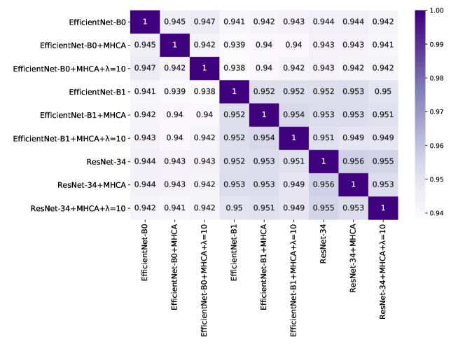
C_{i,j}=\frac{1}{t}\sum_{r=1}^{t}\mbox{Dice}(\hat{Y}_{i,r},\hat{Y}_{j,r}).

By applying Eq. (6) to all possible model pairs formed from $n$ models, we obtain a symmetric correlation matrix $C$ of size $n\times n$ . We illustrate an example of a correlation matrix in Figure 1. The highest correlation is naturally obtained between a model $M_{i}$ and itself. Hence, the values on the diagonal of $C$ are equal to $1$ .

3.2.2. Ensemble Construction Algorithm

Given a set of $n$ models $\mathcal{M}=\{M_{1},M_{2},...,M_{n}\}$ , and the Dice coefficients $D=\{d_{1},d_{2},....,d_{n}\}$ of the $n$ models with respect to the ground-truth validation labels, we start building the ensemble $\mathcal{E}$ by choosing the best available model. Then, in order to add a new model from $\mathcal{M}\setminus\mathcal{E}$ to $\mathcal{E}$ , we select the best model which is also the least correlated with the models currently added to $\mathcal{E}$ . For each remaining model $M_{i}\in\mathcal{M}\setminus\mathcal{E}$ , we determine the correlation score between $M_{i}$ and $\mathcal{E}$ by taking the average of the correlation scores between $M_{i}$ and the models from $\mathcal{E}$ . In addition, we sum up the Dice error $1-d_{i}$ of the model $M_{i}$ to each correlation $C_{i,j}$ , thus giving equal importance to the performance level of $M_{i}$ and the correlation score between $M_{i}$ and $M_{j}$ . Finally, the average score for adding $M_{i}$ to $\mathcal{E}$ is computed as follows:

(7)

C_{i,\mathcal{E}}=\operatorname*{avg}\left((1-d_{i})+C_{i,j}\right),\forall j\;\mbox{such that}\;M_{j}\in\mathcal{E}.

If there are multiple models with an average score equal to the minimum average score at a certain step, we select the best performing model among them and add it to $\mathcal{E}$ . We perform this operation for $k$ steps, where $k$ ( $1\leq k\leq n$ ) is the maximum number of models to be added to the ensemble, i.e. $k$ represents the budget limitation for the ensemble. The whole process is formally described in Algorithm 1.

We emphasize that our ensemble creation strategy does not require any additional learning steps. Moreover, it does not add any running time overhead during inference. Hence, its computational cost at test time is similar to that of the baseline ensemble creation strategy.

4. Experiments

4.1. Data Set

The UW-Madison GI Tract Image Segmentation data set (Lee et al., 2022) contains MRI scans of the abdominal area. The data set comprises a total of $38,496$ slices. There are three annotated organs, namely the stomach, the small bowel and the large bowel. Only $21,906$ out of $38,496$ slices have annotated organs, the rest of the slices showing abdominal regions where these three organs are not seen, thus being completely annotated as background. The size of each slice varies between $234\times 234$ and $384\times 384$ pixels. We split the data set into $80\%$ for training and $20\%$ for testing. We keep $10\%$ of the training data for validation purposes.

4.2. Evaluation Metrics

In order to evaluate the models, we employ two evaluation metrics. Both metrics measure the overlap between the ground-truth and the predicted segmentations. The first measure is the Intersection over Union (IoU). The IoU score between a ground-truth segmentation mask $Y$ and a predicted mask $\hat{Y}$ is defined as:

(8)

\mbox{IoU}(Y,\hat{Y})=\frac{\lvert Y\cap\hat{Y}\rvert}{\lvert Y\cup\hat{Y}\rvert}.

The second evaluation metric is the Dice coefficient between the ground-truth segmentation and the predicted mask, defined as:

(9)

\mbox{Dice}(Y,\hat{Y})=\frac{2\cdot\lvert Y\cap\hat{Y}\rvert}{\lvert Y\rvert+\lvert\hat{Y}\rvert}.

4.3. Implementation Details

We implement the models in PyTorch. Before training the models, we initialize the weights of the backbones with the values pre-trained on ImageNet (Russakovsky et al., 2015). We set the input size to $320\times 384$ , regardless of the chosen encoder. We train each network for $20$ epochs, setting the batch size to $32$ and the learning rate to $10^{-3}$ . We optimize the networks using the loss defined in Eq. (1), employing the Adam optimizer (Kingma and Ba, 2015) to update the parameters of the models.

When integrating the MHCA modules (Georgescu et al., 2023), we keep the optimal hyperparameters specified by the authors, namely the reduction ratio equal to $0.5$ and the number of heads set to $3$ . We add MHCA to the skip connections of the U-Net model. Based on a preliminary evaluation conducted on the validation set, we decided to add MHCA only to the last two skip connection layers. This can be motivated by the fact that the early skip connection feature maps have very few channels.

4.4. Results

Table 1. Dice and IoU scores obtained by individual U-Net model variants based on different backbones (ResNet-34, EfficientNet-B0, EfficientNet-B1), with and without MHCA modules (Georgescu et al., 2023), and alternating between the standard BCE loss and our positively-biased BCE loss with

\mathbf{\boldsymbol{\lambda}=10}

Backbone	MHCA (Georgescu et al., 2023)	$\mathbf{\boldsymbol{\lambda}=10}$	Dice	IoU
ResNet-34	✗	✗	$0.9051$	$0.8774$
	✓	✗	$0.9045$	$0.8769$
	✓	✓	$0.9054$	$0.8780$
EfficientNet-B0	✗	✗	$0.9111$	$0.8836$
	✓	✗	$0.9087$	$0.8814$
	✓	✓	$0.9103$	$0.8830$
EfficientNet-B1	✗	✗	$0.9110$	$0.8843$
	✓	✗	$0.9112$	$0.8844$
	✓	✓	$0.9130$	$0.8860$

Table 2. Comparing the baseline ensemble formed of the top

\mathbf{k}

models with our diversity-promoting ensemble (DiPE), for

\mathbf{k\in\{2,3,...,9\}}

. The last row shows the results when including all nine U-Nets into the ensemble (no budget limitation on the number of models). When

\mathbf{k=9}

, DiPE becomes equivalent with the ensemble based on all models. Best overall scores are highlighted in bold.

#models	Baseline		DiPE (ours)
$\mathbf{(k)}$	Dice	IoU	Dice	IoU
2	$0.9151$	$0.8886$	$0.9125$	$0.8856$
3	$0.9168$	$0.8903$	$0.9175$	$0.8911$
4	$0.9182$	$0.8920$	$0.9185$	$0.8922$
5	$0.9186$	$0.8923$	$0.9188$	$0.8927$
6	$0.9187$	$0.8924$	$0.9196$	$0.8936$
7	$0.9192$	$0.8931$	$0.9196$	$0.8935$
8	$0.9199$	$0.8938$	$\mathbf{0.9201}$	$\mathbf{0.8940}$
All (9)	$0.9199$	$0.8938$	$0.9199$	$0.8938$

4.4.1. Quantitative Results of Individual U-Net Models

We show the results obtained by individual models on the UW-Madison GI Tract Image Segmentation data set in Table 1. We observe that the best performance of $0.9130$ in terms of the Dice coefficient is obtained when the EfficientNet-B1 architecture is used as backbone for the encoder. When using the ResNet-34 encoder, the Dice coefficient drops to $0.9051$ , showing that the encoder capacity can have a significant impact on the results.

When adding the MHCA modules, only the model based on the EfficientNet-B1 backbone obtains an improvement in terms of the IoU and Dice scores. For the other two models, namely EfficientNet-B0 and ResNet-34, the performance drops by a small margin. When introducing the positively-biased BCE loss (with $\lambda=10$ in Eq. (2)), we observe considerable performance gains for the ResNet-34 and EfficientNet-B1 backbones.

4.4.2. Quantitative Results of Ensembles

Starting from the nine individual U-Net models, we evaluate two ensemble creation strategies which have a restricted computational budget. The budget limitation is introduced in terms of the number of models forming each ensemble. In Table 2, we present the results of the baseline ensemble creation strategy (based on selecting the models with the best performance) versus the results of our DiPE strategy. We observe that our method generally surpasses the baseline method, the only exception being when the number of models $k$ is equal to $2$ . We also note that DiPE obtains slightly better results when using only $k=8$ models in the ensemble than the baseline that combines all models ( $0.9201$ versus $0.9199$ in terms of the Dice coefficient). We can also visualize the performance of our approach versus the performance of the baseline method in Figure 2. The figure clearly shows that DiPE produces superior results, for all ${k\in\{3,...,8\}}$ .

Table 3. Ablation results obtained by removing the Dice error (

\mathbf{1-d_{i}}

) with respect to the ground-truth validation labels from Eq. (7).

#models	DiPE w/o $\mathbf{d_{i}}$ (ours)		DiPE (ours)
$\mathbf{(k)}$	Dice	IoU	Dice	IoU
2	$0.9125$	$0.8856$	$0.9125$	$0.8856$
3	$0.9152$	$0.8886$	$0.9175$	$0.8911$
4	$0.9170$	$0.8906$	$0.9185$	$0.8922$
5	$0.9180$	$0.8917$	$0.9188$	$0.8927$
6	$0.9194$	$0.8933$	$0.9196$	$0.8936$
7	$0.9198$	$0.8937$	$0.9196$	$0.8935$
8	$0.9198$	$0.8937$	$0.9201$	$0.8940$

4.4.3. Ablation Results

We perform an ablation study to prove the necessity of adding the Dice error of the model when computing the average correlation score in Eq. (7). We present the corresponding results in Table 3. If we do not take into account the performance of the models with respect to the ground-truth when creating the ensemble, the performance levels of the ensembles with various budgets drop considerably, e.g. from $0.9188$ to $0.9180$ in terms of the Dice coefficient when using $k=5$ models. This can be explained by the fact that a model which is not correlated with the models already included in the ensemble, might also be less correlated with the ground-truth. In other words, its low correlation score with the previously included models is caused by the poor performance level of the respective model. Hence, we observe that the best strategy when creating an ensemble is to take both aspects into account, namely the performance of the new model and its correlation with the models comprising the current ensemble.

4.4.4. Qualitative Results of Ensembles

In Figure 3, we illustrate some qualitative results to compare the baseline ensemble strategy with our DiPE strategy. We show the segmentation masks of the ensembles consisting of $k=5$ models. We notice that DiPE creates an ensemble which produces better segmentation masks than the baseline strategy. From a medical point of view, the comparison between our DiPE method and the ground-truth (produced by physicians specialized in radiology) exhibits very few differences. For example, we particularly observe that DiPE obtains a segmentation of the stomach (second row of Figure 3) that is much closer to the ground-truth segmentation than the baseline method. In fact, the first two rows exemplify the ability of DiPE to identify and differentiate between the stomach and the transverse colon with a better accuracy than the baseline strategy, producing a result close to what the radiologists have annotated. In general, the stomach region is well identified by both methods, with a slight upper hand for our technique. Furthermore, we underline that our method especially excels on the tissues surrounded by larger amounts of fat, such as the small bowel and the mesentery, as seen in the bottom images. We consider that the ability of DiPE to distinguish between the small bowel and the colon is outstanding, being an almost one-to-one match with the ground-truth. Remarkably, the example shown on the fourth row illustrates that our technique does not mistake the loop of small bowel on the right (or the patient’s left) with gastric structures. In summary, our new method offers significantly better results in comparison with the baseline method, but we believe there is still room for improvement in order to reach the full precision of the experimented human eye.

5. Conclusion

In this work, we studied the task of medical image segmentation, specifically focusing our experiments on the segmentation of the stomach, the small bowel and the large bowel. Towards improving the segmentation accuracy, we proposed a bottom-up diversity-promoting ensemble creation strategy that gives equal importance to the accuracy level and the correlation with other models, when adding a new model to the ensemble. Our ablation results showed that using solely the correlation with other models is suboptimal.

In future work, we aim to extend our empirical analysis to more segmentation tasks from the medical domain. We also aim to replace plurality voting with a meta-learner, which could further improve performance.

Acknowledgements

The research leading to these results has received funding from the NO Grants 2014-2021, under project ELO-Hyp contract no. 24/2020.

References

(1)
Alom et al. (2019) Md Zahangir Alom, Chris Yakopcic, Mahmudul Hasan, Tarek M. Taha, and Vijayan K. Asari. 2019. Recurrent residual U-Net for medical image segmentation. Journal of Medical Imaging 6, 1 (2019), 014006.
Baldeon Calisto and Lai-Yuen (2020) Maria Baldeon Calisto and Susana K. Lai-Yuen. 2020. AdaEn-Net: An ensemble of adaptive 2D–3D Fully Convolutional Networks for medical image segmentation. Neural Networks 126 (2020), 76–94.
Chen et al. (2018) Hao Chen, Qi Dou, Lequan Yu, Jing Qin, and Pheng-Ann Heng. 2018. VoxResNet: Deep voxel-wise residual networks for brain segmentation from 3D MR images. NeuroImage 170 (2018), 446–455.
Chen et al. (2021) Jieneng Chen, Yongyi Lu, Qihang Yu, Xiangde Luo, Ehsan Adeli, Yan Wang, Le Lu, Alan L. Yuille, and Yuyin Zhou. 2021. TransUNet: Transformers Make Strong Encoders for Medical Image Segmentation. arXiv preprint arXiv:2102.04306 (2021).
Chen et al. (2022a) Shuai Chen, Zahra Sedghi Gamechi, Florian Dubost, Gijs van Tulder, and Marleen de Bruijne. 2022a. An end-to-end approach to segmentation in medical images with CNN and posterior-CRF. Medical Image Analysis 76 (2022), 102311.
Chen et al. (2022b) Zhang Chen, Zhiqiang Tian, Jihua Zhu, Ce Li, and Shaoyi Du. 2022b. C-CAM: Causal CAM for Weakly Supervised Semantic Segmentation on Medical Image. In Proceedings CVPR. IEEE, 11676–11685.
Ganaie et al. (2022) M.A. Ganaie, Minghui Hu, A.K. Malik, M. Tanveer, and P.N. Suganthan. 2022. Ensemble deep learning: A review. Engineering Applications of Artificial Intelligence 115 (2022), 105151.
Gao et al. (2021) Yunhe Gao, Mu Zhou, and Dimitris Metaxas. 2021. UTNet: A Hybrid Transformer Architecture for Medical Image Segmentation. In Proceedings of MICCAI. Springer, Cham, 61–71.
Georgescu et al. (2023) Mariana-Iuliana Georgescu, Radu Tudor Ionescu, Andreea-Iuliana Miron, Olivian Savencu, Nicolae-Catalin Ristea, Nicolae Verga, and Fahad Shahbaz Khan. 2023. Multimodal Multi-Head Convolutional Attention with Various Kernel Sizes for Medical Image Super-Resolution. In Proceedings of WACV. IEEE.
Gibson et al. (2018) Eli Gibson, Francesco Giganti, Yipeng Hu, Ester Bonmati, Steve Bandula, Kurinchi Gurusamy, Brian Davidson, Stephen P. Pereira, Matthew J. Clarkson, and Dean C. Barratt. 2018. Automatic Multi-Organ Segmentation on Abdominal CT With Dense V-Networks. IEEE Transactions on Medical Imaging 37, 8 (2018), 1822–1834.
Hatamizadeh et al. (2022) Ali Hatamizadeh, Dong Yang, Holger Roth, and Daguang Xu. 2022. UNETR: Transformers for 3D Medical Image Segmentation. In Proceedings of WACV. IEEE, 574–584.
He et al. (2016) Kaiming He, Xiangyu Zhang, Shaoqing Ren, and Jian Sun. 2016. Deep Residual Learning for Image Recognition. In Proceedings of CVPR. IEEE, 770–778.
Hu et al. (2018) Jie Hu, Li Shen, and Gang Sun. 2018. Squeeze-and-Excitation Networks. In Proceedings of CVPR. IEEE, 7132–7141.
Jin et al. (2021) Dakai Jin, Dazhou Guo, Tsung-Ying Ho, Adam P. Harrison, Jing Xiao, Chen-Kan Tseng, and Le Lu. 2021. DeepTarget: Gross tumor and clinical target volume segmentation in esophageal cancer radiotherapy. Medical Image Analysis 68 (2021), 101909.
Kamnitsas et al. (2017) Konstantinos Kamnitsas, Christian Ledig, Virginia F.J. Newcombe, Joanna P. Simpson, Andrew D. Kane, David K. Menon, Daniel Rueckert, and Ben Glocker. 2017. Efficient multi-scale 3D CNN with fully connected CRF for accurate brain lesion segmentation. Medical Image Analysis 36 (2017), 61–78.
Kingma and Ba (2015) Diederik P. Kingma and Jimmy Ba. 2015. Adam: A method for stochastic optimization. In Proceedings of ICLR. arXiv.
Lee et al. (2022) Sangjune Laurence Lee, Poonam Yadav, Yin Li, Jason J. Meudt, Jessica Strang, Dustin Hebel, Alyx Alfson, Stephanie J. Olson, Tera R. Kruser, Jennifer B. Smilowitz, Kailee Borchert, Brianne Loritz, John Bayouth, and Michael Bassetti. 2022. UW-Madison GI Tract Image Segmentation Data Set. https://www.kaggle.com/competitions/uw-madison-gi-tract-image-segmentation/. Accessed: 2022-10-10.
Luo et al. (2021) Xiangde Luo, Guotai Wang, Tao Song, Jingyang Zhang, Michael Aertsen, Jan Deprest, Sebastien Ourselin, Tom Vercauteren, and Shaoting Zhang. 2021. MIDeepSeg: Minimally interactive segmentation of unseen objects from medical images using deep learning. Medical Image Analysis 72 (2021), 102102.
Lyksborg et al. (2015) Mark Lyksborg, Oula Puonti, Mikael Agn, and Rasmus Larsen. 2015. An ensemble of 2D convolutional neural networks for tumor segmentation. In Proceedings of SCIA. Springer, 201–211.
Men et al. (2018) Kuo Men, Pamela Boimel, James Janopaul-Naylor, Haoyu Zhong, Mi Huang, Huaizhi Geng, Chingyun Cheng, Yong Fan, John P. Plastaras, Edgar Ben-Josef, and Ying Xiao. 2018. Cascaded atrous convolution and spatial pyramid pooling for more accurate tumor target segmentation for rectal cancer radiotherapy. Physics in Medicine and Biology 63 (2018), 185016.
Oktay et al. (2018) Ozan Oktay, Jo Schlemper, Loic Le Folgoc, Matthew Lee, Mattias Heinrich, Kazunari Misawa, Kensaku Mori, Steven McDonagh, Nils Y. Hammerla, Bernhard Kainz, et al. 2018. Attention U-Net: Learning where to look for the pancreas. In MIDL. arXiv.
Ronneberger et al. (2015) Olaf Ronneberger, Philipp Fischer, and Thomas Brox. 2015. U-Net: Convolutional Networks for Biomedical Image Segmentation. In Proceedings of MICCAI. Springer, Cham, 234–241.
Russakovsky et al. (2015) Olga Russakovsky, Jia Deng, Hao Su, Jonathan Krause, Sanjeev Satheesh, Sean Ma, Zhiheng Huang, Andrej Karpathy, Aditya Khosla, Michael Bernstein, Alexander C. Berg, and Li Fei-Fei. 2015. ImageNet Large Scale Visual Recognition Challenge. International Journal of Computer Vision 115, 3 (2015), 211–252.
Salehi et al. (2017) Seyed Sadegh Mohseni Salehi, Deniz Erdogmus, and Ali Gholipour. 2017. Tversky Loss Function for Image Segmentation Using 3D Fully Convolutional Deep Networks. In Proceedings of MLMI. Springer, Cham, 379–387.
Seo et al. (2020) Hyunseok Seo, Charles Huang, Maxime Bassenne, Ruoxiu Xiao, and Lei Xing. 2020. Modified U-Net (mU-Net) With Incorporation of Object-Dependent High Level Features for Improved Liver and Liver-Tumor Segmentation in CT Images. IEEE Transactions on Medical Imaging 39, 5 (2020), 1316–1325.
Siddique et al. (2021) Nahian Siddique, Sidike Paheding, Colin P. Elkin, and Vijay Devabhaktuni. 2021. U-Net and Its Variants for Medical Image Segmentation: A Review of Theory and Applications. IEEE Access 9 (2021), 82031–82057.
Tan and Le (2019) Mingxing Tan and Quoc Le. 2019. EfficientNet: Rethinking Model Scaling for Convolutional Neural Networks. In Proceedings of ICML, Vol. 97. PMLR, 6105–6114.
Verga et al. (2014) N. Verga, D.A. Mirea, I. Busca, M.N. Poroschianu, S.F. Zarma, L. Grinisteanu, A. Anica, C.A. Gheorghe, C.A. Stan, M. Verga, and R. Vasilache. 2014. Optical coherence tomography in oncological imaging. Romanian Reports in Physics 66, 1 (2014), 75–86.
Wang et al. (2018) Yan Wang, Chen Zu, Guangliang Hu, Yong Luo, Zongqing Ma, Kun He, Xi Wu, and Jiliu Zhou. 2018. Automatic Tumor Segmentation with Deep Convolutional Neural Networks for Radiotherapy Applications. Neural Processing Letters 48 (2018), 1323–1334.
Wolz et al. (2013) Robin Wolz, Chengwen Chu, Kazunari Misawa, Michitaka Fujiwara, Kensaku Mori, and Daniel Rueckert. 2013. Automated Abdominal Multi-Organ Segmentation With Subject-Specific Atlas Generation. IEEE Transactions on Medical Imaging 32, 9 (2013), 1723–1730.
Woo et al. (2018) Sanghyun Woo, Jongchan Park, Joon-Young Lee, and In-So Kweon. 2018. CBAM: Convolutional Block Attention Module. In Proceedings of ECCV. Springer, Cham, 3–19.
Zhao et al. (2022) Xiangyu Zhao, Peng Zhang, Fan Song, Chenbin Ma, Guangda Fan, Yangyang Sun, Youdan Feng, and Guanglei Zhang. 2022. Prior Attention Network for Multi-Lesion Segmentation in Medical Images. IEEE Transactions on Medical Imaging 41, 12 (2022), 3812–3823.
Zhao et al. (2019) Yuan-Xing Zhao, Yan-Ming Zhang, Ming Song, and Cheng-Lin Liu. 2019. Multi-view Semi-supervised 3D Whole Brain Segmentation with a Self-ensemble Network. In Proceedings of MICCAI. Springer, Cham, 256–265.
Zhou et al. (2019) Yuyin Zhou, Zhe Li, Song Bai, Xinlei Chen, Mei Han, Chong Wang, Elliot Fishman, and Alan L. Yuille. 2019. Prior-aware neural network for partially-supervised multi-organ segmentation. In Proceedings of ICCV. IEEE, 10671–10680.
Zhou et al. (2018) Zongwei Zhou, Md Mahfuzur Rahman Siddiquee, Nima Tajbakhsh, and Jianming Liang. 2018. UNet++: A Nested U-Net Architecture for Medical Image Segmentation. In Proceedings of DLMIA. Springer, Cham, 3–11.