Distributional regression models for Extended Generalized Pareto distributions
Abstract
The Extended Generalized Pareto Distribution (EGPD) (Naveau et al. 2016) is a family of distribution that has been introduced to model the full range of a positive random variable but with the lower and the upper tails distributed according the peaks-over-threshold methodology. The aim of this article is to augment the scope of application of EGPD allowing the analyst to incorporate the effect of covariates on the model. In particular we introduce a specification where the parameters of EGPD can be modeled as additive functions of the covariates, e.g. space or time. As a related product we provide an add-on code written in R that it is flexible enough to implement the EGPD in a generic way, allowing to introduce new parametric forms. We show the potential of our add-on on the modeling of hourly rainfalls over the North-West region of France and discuss modeling strategies.
Keywords: Extreme events, Statistical modeling, Statistical software, Rainfall simulation, Geostatistics
1 Introduction
The Peak Over Threshold (POT) method, described in details by Coles (2001, Chapter 4), has been used in many fields to identify extremal events such as loads, wave heights, floods, wind velocities, etc. This method provides a model for independent exceedances over a high threshold. According the Pickands-Balkema-de Haan theorem (Balkema and De Haan, 1974; Pickands III, 1975) for a threshold sufficiently high, the unnormalized conditional tail distribution of a random variable can be approximated as
where
| (1) |
and .
The limiting distribution (1) is referred to as the Generalized Pareto distribution (GPD) and the parameters and are respectively the shape and the scale parameters. The scale parameter depend on the threshold , but in remainder of the paper the subscript is dropped in the notation.
Modeling using GPD has become very popular since the paper of Davison and Smith (1990) where estimation and model-checking procedures for univariate and regression data are developed. Such procedure have then been extended by allowing the GPD parameters to be represented as smooth functions of covariates (Chavez-Demoulin and Davison, 2005).
Since then several R packages have been developed to fit GPDs and contributed to the Comprehensive R Archive Network (CRAN) in the field of extreme value analysis (R Core Team, 2022). Among them, ismev (Heffernan et al., 2018), providing tools for the extreme value analyses presented in Coles (2001), evd (Stephenson, 2002), evir (Pfaff and McNeil, 2018), extRemes (Gilleland and Katz, 2016) and mev (Belzile et al., 2020), have offered various approaches for fitting univariate and multivariate GPDs. Gilleland et al. (2013) and, more recently, Belzile et al. (2022) review them while the Dutang and Jaunatre (2022)’s CRAN Task View provides an up-to-date list of the R packages in this field. In particular, some of them offer regression-based models for extreme distributions, where GPD parameters are allowed to vary with covariates. Beyond the linear forms introduced in the packages ismev and evd, a few R packages allow to fit GPDs with parameters following additive forms i.e. when the parameters or their transformations can be modelled as additive smooth functions of the covariates. In the sequel we term this form a Generalized Additive Model (GAM) (Hastie and Tibshirani, 1990; Wood, 2017). Thus VGAM (Yee and Stephenson, 2007), gamlss (Rigby and Stasinopoulos, 2005) and evgam (Youngman, 2020) provide this functionality for GPDs, as reviewed among other alternatives in Youngman (2020).
It is clear that GPD needs the determination of a threshold which is neither too high. The choice of an appropriate threshold is challenging because the stability plots and the mean residual life (Coles, 2001, Chapter 4) plot do not give an obvious value of a suitable threshold. The problem is tackled in a regression setting by Eastoe and Tawn (2009). However the question of the threshold choice and then simulation of the whole spectrum of the random variable considered remains problematic.
Forming mixtures of Exponential distributions (Wilks, 1998; Keller et al., 2015) or conditional Gamma distributions (Kenabatho et al., 2012; Chen et al., 2014) remains a competitive alternative e.g. for heavy-tailed precipitation modeling and simulation. Approaches of this type are implemented in the package GSM, that uses a Bayesian approach for estimating a mixture of Gamma distributions in which the mixing occurs over the shape parameter and the procedure only requires to specify a prior distribution for a single parameter. The package evmix fits an extreme value mixture model with normal behavior for the bulk distribution up to the threshold and conditional GPD above the threshold. Options for profile likelihood estimation for threshold and fixed threshold approach are provided. Finally, distributionsrd provides the double Pareto-lognormal distribution.
Although interesting, in practice these packages do not allow to fit nonlinear models as flexible as the GAM options allowed for the GPD alone. Besides, the mixture approaches tend to quickly inflate the number of parameters and the inference of the latter may be problematical operationally (Naveau et al., 2016).
Papastathopoulos and Tawn (2013) opened another route in the field of heavy-tail distribution modeling by replacing the uniform draws in the inverse cumulative distribution function (CDF) transform to generate simulations of the GPD, by draws from a richer distribution e.g. type Beta distribution. Using this approach, Naveau et al. (2016) presented a concise parametric formulation (later extended to a semi-parametric formulation (Tencaliec et al., 2020)) for simulating the whole range of a positive random variable (namely precipitations), that makes use of GPD to model not only the high quantiles but the smallest ones as well and bypass the issue of threshold selection. The main idea rooted from composing a cumulative distribution function with the GPD (see section 2 for more details). Very recently, a similar idea was taken up by Stein (2021a, b).
In the sequel, we refer to the extension of GPD in the sense of Naveau et al. (2016) as Extended Generalized Pareto distribution (EGPD). An implementation of EGPD with four parametric families, together with the fitting procedure, can be found in the R package mev.
The aim of this work is to extend the applicability of the EGPD in the presence of covariates that can modify the parameters of the distribution. The extension takes place in the same spirit as GAM. We also want to present an add-on to the gamlss package that allows to make inference on the parameter.
We have chosen the gamlss package because it provides univariate distributional regression models, where parameters of the assumed distribution for the response can be modeled as additive functions of the covariates. It is flexible enough to allow the encoding of novel families of distribution, as long as their density, cumulative, quantile and random generative function and, optionally, first and second (cross-) derivatives of the likelihood can be computed. We seize this potential to implement the parametric EGPD family in a generic way, allowing to introduce new parametric forms, up to 4 parameters so far (due to limitations of gamlss), satisfying the requirement of the EGPD family.
The remaining of this article will first introduce the EGPD and the distribution regression model (Section 2), followed by the key commands to use the EGPD within the gamlss package and our add-on in Section 3. Section 4 implements them to perform an analysis of hourly positive rainfalls on the North-west of France and discuss specific advantages and limitations of distributional regression modeling and its implementation in R, while Section 5 concludes the paper.
2 A distributional regression model
2.1 Extended-GPD
The EGPD (Naveau et al., 2016) accounts simultaneously and in a parsimonious way for both extreme and non extreme values of a random variable . Its cumulative distribution function (CDF) reads:
| (2) |
The function is a continuous CDF on the unit interval. It is constrained by several assumptions: 1) we need to ensure that the upper-tail behavior of follows a GPD; 2) the low values of , seen as the upper tail of when , follows a GPD as well.
This leads to the following consequences for any candidate CDF :
-
a.
the upper-tail behavior of is equivalent to the original GPD tail used to build ;
-
b.
when , where is positive and finite for some real .
Four parametric families, , , that satisfies the above-mentioned constraints are proposed in Naveau et al. (2016).
-
1.
,
-
2.
, and
-
3.
, where is the CDF of a Beta random variable with parameters and , that is:
-
4.
,
In model 1, controls the rate of upper tail decay, the shape of the lower tail and is a scale parameter. allows us to recover the GPD model, while varying it gives flexibility in the description of the lower tail.
Model 2, as a mixture of power laws, allows to increase the flexibility provided by model 1. Therein, controls the lower tail behavior while modifies the shape of the density in its central part.
Model 3 is connected to the work of Falk et al. (2010). keeps controlling the upper extreme tail, the central part of the distribution in a threshold tuning way. However, this model imposes a behavior type for the lower tail (null density at ) instead of allowing the data to constrain it.
Hence Model 4, which adds an extra parameter to circumvent this limitation. In this last model, control respectively the lower, moderate and upper parts of the distribution. By construction, the lower and upper tails are GPD of shape parameters and respectively.
In the sequel we denote the vector of parameters with and the density of a parametrized EGPD with . To simulate from Equation (2), the user randomly draws a uniform variable in and then applies the quantile function , given for by:
| (3) |
2.2 Additive model specification
In practice, the parameters of the distribution of may depend on some covariates , i.e.
| (4) |
where . The previous specification is an instance of a distributional regression model (Stasinopoulos et al., 2018).
For relating the different distributional parameters to the covariates, we rely on additive predictors of the form
| (5) |
where are smooth functions of the covariates .
The representation (5) is particularly flexible and allows to capture complex dependence patterns between distribution parameters and covariates . For instance a semiparametric model with two covariates can be written as
Another example is when we want to model space-time data observed at site and at time . In this case
In analogy to Generalized Linear Model the predictors are linked to the distributional parameters via known monotonic and twice differentiable link functions .
In the case of model 1, i.e. , common link functions are
| (6) |
The functions in (5) are approximated in terms of basis function expansions
| (7) |
where are the basis functions and denote the corresponding basis coefficients. These basis can be of different types, thoroughly presented e.g. in Stasinopoulos et al. (2017) or Wood (2017).
The basis function expansions can be written as
where is still a vector of transformed covariates that depends on the basis functions. and is a parameter vector to be estimated.
To ensure regularization of the functions so-called penalty terms are added to the objective log-likelihood function. Usually, the penalty for each function are quadratic penalty where is a known semi-definite matrix and the vector regulates the amount of smoothing needed for the fit. A special case is when . Therefore the type and properties of the smoothing functions are controlled by the vectors and the matrices .
The penalized log-likelihood function for the latter models reads:
| (8) |
where represents the log-likelihood function for the model (4).
3 Distributional regression model for EGPD within the R package gamlss
In this section we introduce an add-on script in R that implements the EGPD regression model described in the previous section. The script, available in github.com/noemielc/egpd4gamlss, is flexible enough as it only requires the specification of a parametric CDF .
The Generalized Additive Model for Location, Scale and Shape (GAMLSS) is an example of distributional regression model and the companion package in R gamlss (Stasinopoulos et al., 2017) allows a straightforward fitting of multiple built-in and well-known family distributions with parameters that vary flexibly with as in (5)-(6).
An interesting feature is the possibility to extend the family of distributions described in Rigby et al. (2019). The only limitation is the dimension of the parameter vector , , where the four parameters are denoted with , , and in gamlss.
Due to the restriction on the number of parameters, our code allows the implementation of parametric distributions for with only 2 parameters, namely . In the following, the parameters of the EGPD distribution are identified with .
The generic implementation of a EGPD is provided in the file GenericEGPDg.R. The MakeEGPD function assembles a new EGPD family distribution exploiting an user-built as a function of and (at most) two parameters and . The required first, second and cross derivatives of the density in (4), necessary for the fitting procedure in gamlss, are obtained by the symbolic derivation using the R package Deriv. Moreover the inverse function is computed numerically.
In the following, we exemplify the use of MakeEGPD by assembling Model 1, .
The last command is necessary and allows to create the object EGPDModel1 (name concatenating EGPD and Gname) from the EGPD1Family function.
For given values and , the R functions of density, cumulative distribution function, quantile function and random generation are ready to use.
The reserved names for the distribution parameters in gamlss are mu (), sigma (), nu (), and tau (). To change the link functions by means of which each EGPD parameter (here or ) is indirectly optimised, or the default starting values for the parameters to fit, or to print these links, we use the commands:
It is possible to create an original link function ”own”, by gathering the expressions of the link function , its inverse, the derivative of the latter w.r.t. parameter and its area of validity. For instance to create a log-link function shifted to the right for :
For more details on link function definition, we refer to Stasinopoulos et al. (2017, pag. 179).
4 Application to a hourly rainfall dataset in France
4.1 Data
We illustrate our add-on to package gamlss with the analysis of the hourly precipitations recorded over the north-west area of France from 2016 to 2018 both included. This database, containing precipitations as well as other meteorological variables whose values are registered every 6 minutes over the 3 years of interest for each of the 274 stations of the network (see Figure 1), is freely accessible (see Larvor et al., 2020, fro more details).
Let us note the random variable for strictly positive hourly precipitations (dry and wet events are traditionally treated separately when it comes to rainfall simulation (Ailliot et al., 2015)), with covariates , where and represents the position in space (longitude, latitude) and a cyclic time index, namely the day or the month of the year. The work of Naveau et al. (2016) and our tests show that EGPD fitting is improved by censoring the data, so in practice we remove values (mm). Other thresholds ( and mm) have been tested but (mm) gives the best results, in particular for the upper tails. Besides, as noted in Evin et al. (2018); Naveau et al. (2016), negative shape parameters are not expected for rainfall distributions at these time scales, so we use a link function constraining the parameter to positive values. Finally, as performed in Naveau et al. (2016), we only keep one every three hourly records of precipitation so as to ensure independency between samples.
4.2 Model fitting
We fit different specifications of EGPD-based models, where EGPD takes form 1, 3 or 4, and compare them with equivalently specified Gamma-based models. The Gamma (GA) distribution is a classical choice that works well for modeling the bulk of precipitations at a given site (Katz, 1977; Vrac and Naveau, 2007; Vlček and Huth, 2009). However non-negligible deviations are observed when one is interested in capturing extreme rainfalls (Katz et al., 2002), typically underestimated due to the lightness of the GA tail. For a marginal model M=EGPD1,EGPD3,EGPD4,GA, the different specifications read:
-
M.0 where
i.e. the parameters do not depend on the covariates ;
-
M.t where
uses cyclic cubic splines to model the nonlinear dependency in time while considering no variation in space ;
-
M.tnomu where
does the same as before but considers as constant the parameter ;
-
M.st where
uses smooth surface fitting (thin-plate splines) to model the dependency in space as well as cyclic cubic splines for the dependency in time ;
-
M.st2mu where
does the same as before but considers constant in space the parameters that are not or ;
-
M.st2nomu where
does the same as before but considers constant in space the parameters and ;
-
M.st3nomu where
does the same as before but applies to M=EGPD4 only and considers parameter as a constant over space.
These variations within each model class will allow us to assess whether the smooth regression of distribution parameters over covariates is justified or not. Below we reproduce the code to fit megpd1.0, megpd1.tnomu and mga.st on the training set (training), that contains 60 % of the stations, as reported on Figure 1. The dataset consisting of the remaining stations form the validation set (validation). The gamlss() function reads:
4.3 Model assessment
In order to evaluate the goodness of fit on the training set, we use summary statistics: Global Deviance (GD), Akaike Information Criterion (AIC) and Bayesian Information Criterion (BIC). The GAIC(modelName,k=a) function allows to compute GD (minus twice the fitted log-likelihood, ), the AIC () and the BIC () for each fitted model modelName and to compare them as performed on Figure 2. Besides, Table 1 indicates the effective degree of freedom (df) computed for each model. The function call is reproduced below for the models of class EGPD1.

| Model | df |
|---|---|
| megpd4.st | 242.0 |
| megpd4.st3nomu | 199.3 |
| megpd4.st2nomu | 138.3 |
| megpd4.st2mu | 122.5 |
| megpd4.t | 72.0 |
| megpd4.tnomu | 38.0 |
| megpd4.0 | 4 |
| megpd1.st | 183.0 |
| megpd1.st2nomu | 139.3 |
| megpd1.st2mu | 121.3 |
| megpd1.t | 54.0 |
| megpd1.tnomu | 37.0 |
| megpd1.0 | 3 |
| megpd3.st | 181.6 |
| megpd3.st2nomu | 137.3 |
| megpd3.st2mu | 122.9 |
| megpd3.t | 54.0 |
| megpd3.tnomu | 37.0 |
| megpd3.0 | 3 |
| mga.st | 120.2 |
| mga.stnomu | 78.0 |
| mga.t | 36.0 |
| mga.0 | 2 |


From Figure 2, we can see that, as could be expected, for each classes of models (where EGPD1-based models represent one class, EGPD3-based ones another, etc) the GD ranks first models with the full space-time description M.st. All other variations are rather close in fitting performance, at the exception of the constant-parameters one M.0, that is largely behind. This shows the clear interest of allowing a smooth variation of distribution parameters as a function of the chosen covariates. However, when it comes to modeling efficiency, where the trade-off between number of parameters and performances is taken into account (through the AIC and BIC), the full space-time model M.st becomes much less desirable, falling just above and occasionally behind the constant parameter models M.0. This is all the more through that we consider the BIC indice, that penalizes more the number of parameters than the AIC, and a model with a large number of parameters (EGPD4 versus GA). The best trade-off, according to the BIC, are the time-only full model M.t for the GA class and the time-only without the shape parameter otherwise. This may also be an indication that the seasonal variation of distribution parameters is more important than their spatial variation over the area of interest.
The ranking of model variations within a same model class allows us to draw conclusions w.r.t. the advantages or challenges of each class. Thus, for EGPD4 the GD ranks model variations following decreasing complexity: megpd4.st followed by megpd4.st3nomu, etc. We can deduce that the estimation of is not that sensitive when it comes to the fitting set (at least with enough data). On the contrary, megpd1.st2nomu is preferred to megpd1.st and megpd1.st2mu which can be interpreted as being a rather sensitive parameter to estimate for EGPD1. Considering it constant in space consequently improves the global fitting.
Performances on the validation set are obtained by means of the getTGD() and TGD() functions, providing the validation global deviance (GD-v), that is the GD evaluated using predictive values for the parameters at the validation sample.
Thus, when it comes to extrapolating parameters for new covariate values, the GD-v ranking displayed in Figure 2 reveals that models considering only the dependence in time (M.t, M.tnomu) are systematically preferred, followed by space-time models not considering (M.st2nomu), before the full space-time models (M.st). This supports the fact that the rainfall distributions are relatively close over the studied geographical area, compared to their time evolution that shows stronger variations. Consequently, given the limited size of the dataset, keeping low the number of parameters to regress on covariates (by considering the seasonality only) and in particular avoiding in this category the shape parameter , makes estimations more robust. This agrees with observations from Evin et al. (2018), who noted that fitting the shape parameter is the most challenging part of (extended)-GPD modeling. They concluded that mono-site fitting is not robust, leading e.g. to negative shape parameters that do not match observations on rainfall intensities. To circumvent this issue, the authors use constant parameters within regions of influence defined by homogeneity tests.
4.3.1 Model verification and comparison


Now that it is admitted that regressing distributional parameters over time and possibly space is justified for the case study at hand, we want to assess how good is the modeling and compare model classes at hand. A way to verify whether the fitted models actually represents well the empirical distribution is to draw so-called P-P plots. A simple result in probability states if then is uniformly distributed on the unit interval.
Therefore we can consider the residuals where are the parameters of the fitted model and, after having ordered them, compare them with . Here is the number of observations at hand. The closer points are to the diagonal, the better the model fit. Results are broken down at each season for model variations M.st2nomu on the verification set in Figure 3. They show that at all seasons, EGPD4 outperforms the other models. This is all the more true that we consider not too small rainfalls, namely hourly amounts mm. Below, we keep wiggly artefacts of the discrete sampling scale of observations. Indeed, rainfall amounts are sampled with a precision of mm, which makes the distribution of small values more discrete than continuous. Behind, come models GA, EGPD3 and finally EGPD1. EGPD3 is often better than GA for small hourly rain amounts (below around mm) however it may be outperformed for larger ones, especially in winter. EGPD1 performs as EGPD3 for intermediate and large amounts of rain, but is significantly behind all other models for small amounts.
4.3.2 Visualisation of the fitted functions


Figure 4 represents the fitted functions for the variations megpd4.0 (constant parameters), megpd4.t (smooth time dependence only), and megpd4.st (full smooth space time dependence) of the EGPD4 model in two a priori rather different stations when it comes to the rainfall regime: the north-west coast of Brittany ( ) and the south-east countryside of our area of interest ( ).
The functions predict() or predictAll() are used to provide fitted values of the functions of the covariates. Standard errors can be extracted for fitted values by means of the argument se.fit=TRUE. However this option is not supported by gamlss for parameter estimates on new covariate values at the moment of writing this paper.
We observe rather similar temporal behaviors of the parameters estimated in both stations, highlighting the relative spatial homogeneity of distributions compared to their seasonal dependence. The standard errors decrease with the simplicity of the model ; they are generally negligible for for parameters and but can become significant for parameters and when we are dealing with space-time models. Beyond that, the estimations for the three different versions of the EGPD4-based model are consistent. We note (second station) that a shift between megpd4.t and megpd4.st’s estimates of parameter is compensated by an opposite shift between the associated estimates of parameter . From our observations and experience on EGPD fitting, a given EGPD-based distribution is matched by several local optima (i.e. parameter combinations). Along this ”Pareto front”, is increasing for EGPD1 when decreases. Similarly is increasing for EGPD4 when decreases.


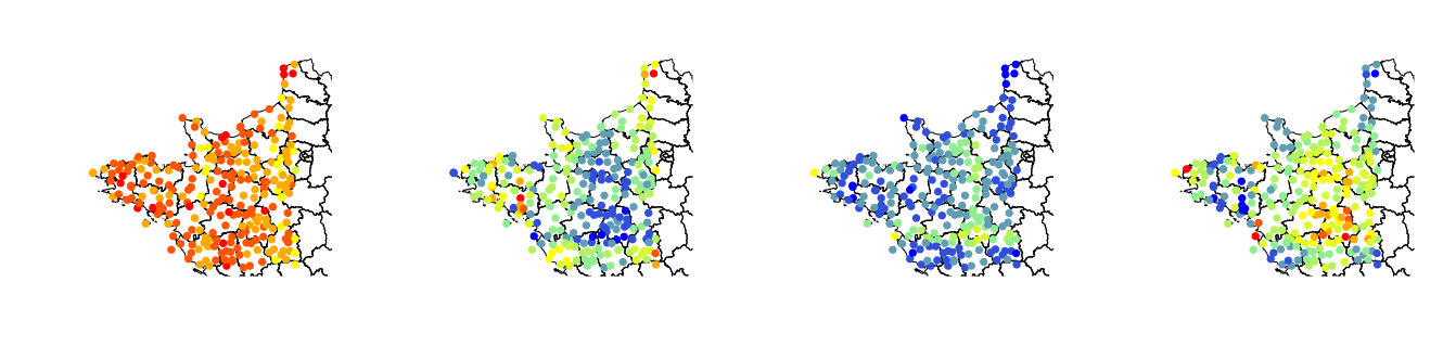
Finally, Figure 5 represents the spatial distribution of the median of the EGPD4 parameters estimated from megpd4.st at three different times of the year: december, april and august. We indeed observe spatial variations of the parameter values, in addition to the monthly changes already discussed. the most spatially homogeneous parameter, which goes in line with previous observations that favored spatially constant -models over non-constant ones. We also note that the map follows an opposite trend w.r.t. ’s map: the larger , the smaller , which follows the general idea of parameter Pareto front developed earlier.
4.3.3 Goodness-of-fit w.r.t. the upper tail
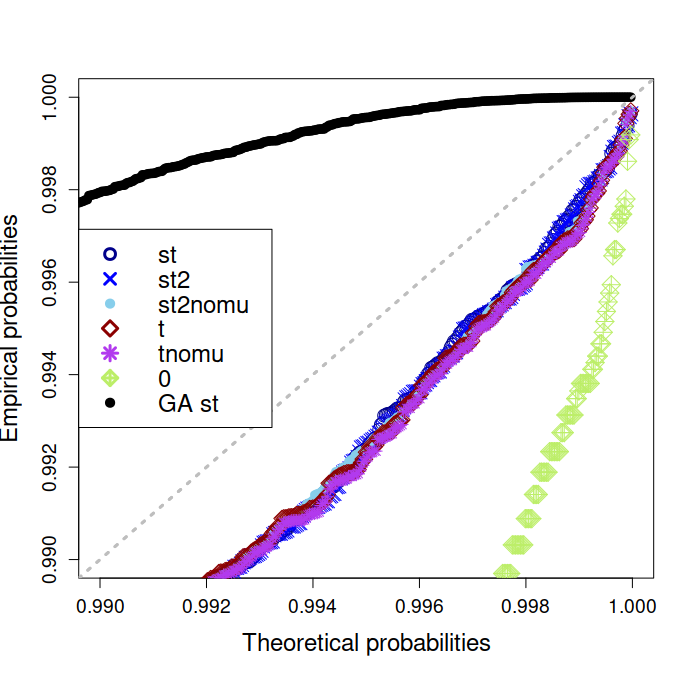


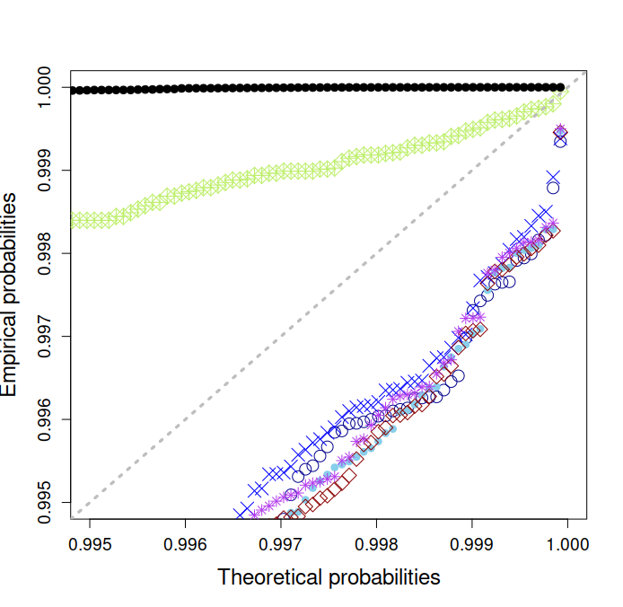


We finish the presentation of the results by comparing in Figure 6 the EGPD4 model to a GA fit, for all stations of the validation set and for each season. We want to check the added value of the EGPD4 model over the GA when it comes to extremes, as well as to assess the best modeling option for the EGPD4 shape parameter in order to ensure a correct representation of extremes. The series of P-P plots presented on Figure 6 focus on the upper tail of the distribution (above the quantiles 0.99 and 0.995 respectively) and allow us to do that. We first note that whatever the season, EGPD4 performs significantly better than GA when it comes to extremes. Most often, the constant parameter model megpd4.0 is enough to outperform the GA, and sometimes is clearly the best option as in spring and autumn. In winter and summer, it is not enough to capture correctly the upper tail of the empirical distribution. Making EGPD4 parameters dependent on time only is sufficient to obtain correct upper tail representations, whether is considered constant (megpd4.tnomu) or not (megpd4.t). The difference between the last two models is very small however using the constant shape parameter option can slightly improve results, especially for larger quantiles (0.995 and above versus 0.99). Adding spatial dependence to the temporal one improves even more the accuracy of the EGPD4 upper tail modeling. Making spatially dependent only two parameters usually performs better. However needs to be included in these two parameters (megpd4.st2 versus megpd4.st2nomu). This highlights the fact that a smooth space-time estimation of the shape parameter is important to capture correctly the non-stationary behavior of the upper tail of the rainfall distributions. However, due to limited data and numerical sensitivity of that estimation, it may be preferable to only limit the smooth spatial dependence to two parameters instead of four, including , in order to make it more robust for extrapolation.
5 Conclusions
This article introduced an add-on to the R-package gamlss, to model non-stationary fields whose margins are EGPD distributed. A number of R packages target the modeling of heavy-tailed distributions. Yet, although some allow distributional regression models, for which distribution parameters can be modeled as additive functions of covariates, none of these packages address the extended-GPD distribution nor another form of unique and closed-form formulation for heavy-tailed distributions that models small, intermediate and large values in a synthetic manner. This add-on implements the EGPD family in a generic way in the gamlss package, allowing to test any new parametric form, up to 4 parameters so far, satisfying the requirement of the EGPD family. Applications include space-time modeling of rainfall marginal distributions. The example developed in this paper shows 1) that modeling hourly rainfall amounts is significantly improved when distribution parameters are non-stationary in space and time; and that 2) the EGPD class clearly improves the modeling of intermediate values and upper tail compared to a classical Gamma option. This illustrates the benefits of our add-on with respect to existing GAM forms for modeling non-stationary margins (typically the Gamma model for our application). We compare three parametric EGPD models and discuss the modeling strategies to best capture non stationary upper tails with limited datasets. This case study also reveals the added-value of EGPD4 (and to a less extent EGPD3) over EGPD1 to correctly model hourly rainfall distributions in a space-time context, while previous works Naveau et al. (2016); Evin et al. (2018); Bertolacci et al. (2018) restricted themselves to EGPD1 as the best option.
Software and data availability
The add-on to the R-package gamlss (Stasinopoulos et al., 2022) presented here for the generic implementation of EGPD consists in the script GenericEGPDg.R, available at https://github.com/noemielc/egpd4gamlss. On this same webpage, supplementary material consisting in a reproducible tutorial with code is presented.
The data used in this paper is freely accessible on the MeteoNet French database (Larvor et al., 2020): https://meteofrance.github.io/meteonet/english/data/summary/
Acknowledgement
Scientific activity was performed as part of the research program Venezia2021, coordinated by CORILA, with the contribution of the Provveditorato for the Public Works of Veneto, Trentino Alto Adige and Friuli Venezia Giulia (Italy). The authors thank Nicolas Berthier for helpful R suggestions.
References
- Ailliot et al. (2015) Ailliot, P., Allard, D., Monbet, V., Naveau, P., 2015. Stochastic weather generators: an overview of weather type models. Journal de la Société Française de Statistique 156, 101–113.
- Balkema and De Haan (1974) Balkema, A.A., De Haan, L., 1974. Residual life time at great age. The Annals of Probability 2, 792–804.
- Belzile et al. (2020) Belzile, L., Wadsworth, J.L., Northrop, P.J., Grimshaw, S.D., Huser, R., 2020. mev: Multivariate Extreme Value Distributions. URL: https://CRAN.R-project.org/package=mev. r package version 1.13.1.
- Belzile et al. (2022) Belzile, L.R., Dutang, C., Northrop, P.J., Opitz, T., 2022. A modeler’s guide to extreme value software. URL: https://arxiv.org/abs/2205.07714.
- Bertolacci et al. (2018) Bertolacci, M., Cripps, E., Rosen, O., Cripps, S., 2018. A comparison of methods for modeling marginal non-zero daily rainfall across the Australian continent. arXiv preprint arXiv:1804.08807 .
- Chavez-Demoulin and Davison (2005) Chavez-Demoulin, V., Davison, A.C., 2005. Generalized additive modelling of sample extremes. Journal of the Royal Statistical Society: Series C (Applied Statistics) 54, 207–222.
- Chen et al. (2014) Chen, J., Brissette, F.P., Zhang, X.J., 2014. A multi-site stochastic weather generator for daily precipitation and temperature. Transactions of the ASABE 57, 1375–1391.
- Coles (2001) Coles, S., 2001. An Introduction to Statistical Modeling of Extreme Values. Springer, New York.
- Davison and Smith (1990) Davison, A.C., Smith, R.L., 1990. Models for exceedances over high thresholds. Journal of the Royal Statistical Society: Series B (Methodological) 52, 393–425.
- Dutang and Jaunatre (2022) Dutang, C., Jaunatre, K., 2022. CRAN task view: extreme value analysis. Technical Report. Version 2022-02-08, URL https://CRAN. R-project. org/view= ExtremeValue.
- Eastoe and Tawn (2009) Eastoe, E., Tawn, J., 2009. Modelling non-stationary extremes with application to surface-level ozone. Journal of the Royal Statistical Society: Series C (Applied Statistics) 58, 25–45.
- Evin et al. (2018) Evin, G., Favre, A.C., Hingray, B., 2018. Stochastic generation of multi-site daily precipitation focusing on extreme events. Hydrology and Earth System Sciences 22, 655–672.
- Falk et al. (2010) Falk, M., Hüsler, J., Reiss, R.D., 2010. Laws of Small Numbers: Extremes and Rare Events. Springer, Basel.
- Gilleland and Katz (2016) Gilleland, E., Katz, R.W., 2016. extRemes 2.0: an extreme value analysis package in R. Journal of Statistical Software 72, 1–39.
- Gilleland et al. (2013) Gilleland, E., Ribatet, M., Stephenson, A.G., 2013. A software review for extreme value analysis. Extremes 16, 103–119.
- Hastie and Tibshirani (1990) Hastie, T.J., Tibshirani, R.J., 1990. Generalized Additive Models. Chapman & Hall/CRC.
- Heffernan et al. (2018) Heffernan, J.E., Stephenson, A.G., Gilleland, E., 2018. ismev: An introduction to statistical modeling of extreme values. URL: https://CRAN.R-project.org/package=ismev. r package version 1.42.
- Katz (1977) Katz, R.W., 1977. Precipitation as a chain-dependent process. Journal of Applied Meteorology 16, 671–676.
- Katz et al. (2002) Katz, R.W., Parlange, M.B., Naveau, P., 2002. Statistics of extremes in hydrology. Advances in Water Resources 25, 1287–1304.
- Keller et al. (2015) Keller, D.E., Fischer, A.M., Frei, C., Liniger, M.A., Appenzeller, C., Knutti, R., 2015. Implementation and validation of a wilks-type multi-site daily precipitation generator over a typical alpine river catchment. Hydrology and Earth System Sciences 19, 2163–2177.
- Kenabatho et al. (2012) Kenabatho, P.K., McIntyre, N., Chandler, R., Wheater, H., 2012. Stochastic simulation of rainfall in the semi-arid Limpopo basin, Botswana. International Journal of Climatology 32, 1113–1127.
- Larvor et al. (2020) Larvor, G., Berthomier, L., Chabot, V., Le Pape, B., Pradel, B., Perez, L., 2020. MeteoNet, an open reference weather dataset by METEO FRANCE. https://meteofrance.github.io/meteonet/english/data/summary/. Accessed: 2022-02-16.
- Naveau et al. (2016) Naveau, P., Huser, R., Ribereau, P., Hannart, A., 2016. Modeling jointly low, moderate, and heavy rainfall intensities without a threshold selection. Water Resources Research 52, 2753–2769.
- Papastathopoulos and Tawn (2013) Papastathopoulos, I., Tawn, J.A., 2013. Extended generalised Pareto models for tail estimation. Journal of Statistical Planning and Inference 143, 131–143.
- Pfaff and McNeil (2018) Pfaff, B., McNeil, A., 2018. evir: Extreme Values in R. URL: https://CRAN.R-project.org/package=evir. r package version 1.7-4.
- Pickands III (1975) Pickands III, J., 1975. Statistical inference using extreme order statistics. The Annals of Statistics , 119–131.
- R Core Team (2022) R Core Team, 2022. R: A Language and Environment for Statistical Computing. R Foundation for Statistical Computing. Vienna, Austria. URL: https://www.R-project.org/.
- Rigby and Stasinopoulos (2005) Rigby, R.A., Stasinopoulos, D.M., 2005. Generalized additive models for location, scale and shape. Journal of the Royal Statistical Society: Series C (Applied Statistics) 54, 507–554.
- Rigby et al. (2019) Rigby, R.A., Stasinopoulos, M.D., Heller, G.Z., De Bastiani, F., 2019. Distributions for modeling location, scale, and shape: Using GAMLSS in R. CRC press.
- Stasinopoulos et al. (2022) Stasinopoulos, M., Rigby, B., Voudouris, V., Akantziliotou, C., Enea, M., Kiose, D., 2022. gamlss: Generalised additive models for location scale and shape. https://cran.r-project.org/web/packages/gamlss/index.html. Accessed: 2022-07-12.
- Stasinopoulos et al. (2018) Stasinopoulos, M.D., Rigby, R.A., Bastiani, F.D., 2018. GAMLSS: A distributional regression approach. Statistical Modelling 18, 248–273.
- Stasinopoulos et al. (2017) Stasinopoulos, M.D., Rigby, R.A., Heller, G.Z., Voudouris, V., De Bastiani, F., 2017. Flexible regression and smoothing: using GAMLSS in R. CRC Press.
- Stein (2021a) Stein, M.L., 2021a. A parametric model for distributions with flexible behavior in both tails. Environmetrics 32, e2658.
- Stein (2021b) Stein, M.L., 2021b. Parametric models for distributions when interest is in extremes with an application to daily temperature. Extremes 24, 293–323.
- Stephenson (2002) Stephenson, A.G., 2002. evd: Extreme value distributions. R news 2, 31–32.
- Tencaliec et al. (2020) Tencaliec, P., Favre, A.C., Naveau, P., Prieur, C., Nicolet, G., 2020. Flexible semiparametric generalized pareto modeling of the entire range of rainfall amount. Environmetrics 31, e2582.
- Vlček and Huth (2009) Vlček, O., Huth, R., 2009. Is daily precipitation Gamma-distributed ?: Adverse effects of an incorrect use of the Kolmogorov–Smirnov test. Atmospheric Research 93, 759–766.
- Vrac and Naveau (2007) Vrac, M., Naveau, P., 2007. Stochastic downscaling of precipitation: From dry events to heavy rainfalls. Water Resources Research 43.
- Wilks (1998) Wilks, D., 1998. Multisite generalization of a daily stochastic precipitation generation model. journal of Hydrology 210, 178–191.
- Wood (2017) Wood, S.N., 2017. Generalized Additive Models: An Introduction with R. CRC press.
- Yee and Stephenson (2007) Yee, T.W., Stephenson, A.G., 2007. Vector generalized linear and additive extreme value models. Extremes 10, 1–19.
- Youngman (2020) Youngman, B.D., 2020. evgam: An R package for Generalized Additive extreme value models. URL: https://arxiv.org/abs/2003.04067.