Distribution-free inference with hierarchical data
Abstract
This paper studies distribution-free inference in settings where the data set has a hierarchical structure—for example, groups of observations, or repeated measurements. In such settings, standard notions of exchangeability may not hold. To address this challenge, a hierarchical form of exchangeability is derived, facilitating extensions of distribution-free methods, including conformal prediction and jackknife+. While the standard theoretical guarantee obtained by the conformal prediction framework is a marginal predictive coverage guarantee, in the special case of independent repeated measurements, it is possible to achieve a stronger form of coverage—the “second-moment coverage” property—to provide better control of conditional miscoverage rates, and distribution-free prediction sets that achieve this property are constructed. Simulations illustrate that this guarantee indeed leads to uniformly small conditional miscoverage rates. Empirically, this stronger guarantee comes at the cost of a larger width of the prediction set in scenarios where the fitted model is poorly calibrated, but this cost is very mild in cases where the fitted model is accurate.
1 Introduction
Consider a prediction problem where we have training data , and a new observation for which we need to predict its response, . The task of distribution-free prediction is to construct a prediction band satisfying
| (1) |
with respect to data , for any distribution . Methods such as conformal prediction (Vovk et al., 2005) provide an answer to this problem whose validity does not depend on any assumptions on —and indeed, validity holds more generally for any exchangeable data distribution (with i.i.d. data points being an important special case).
Though the marginal coverage guarantee (1) guarantees an overall quality of the prediction set, it is often more desired to have a useful guarantee with conditional coverage
to ensure that the prediction is accurate conditional on the specific feature values of the test point. However, achieving distribution-free conditional coverage is a much more challenging problem. In case of nonatomic features (i.e., where the distribution of has no point masses, such as a continuous distribution), Vovk et al. (2005); Lei and Wasserman (2014); Barber et al. (2021a) prove fundamental limits on the possibility of constructing this stronger type of prediction interval—indeed, in the case of a real-valued response , any such cannot have finite width.
In this work, we study a different setting where the data sampling mechanism is hierarchical, rather than i.i.d.—this builds on the work of Dunn et al. (2022) (detailed below), who also studied conformal prediction in the hierarchical setting. We develop an extension of conformal prediction that works for such data structure, which we denote as hierarchical conformal prediction (HCP), to provide distribution-free marginal predictive coverage in this non-i.i.d. setting. Furthermore, we also explore an important special case, where our data set contains multiple observations (multiple draws of ) for each individual (for each draw of ); in this setting, we propose a variant of our method, HCP2, that moves towards conditional coverage via a stronger “second-moment coverage” guarantee.
1.1 Problem setting: hierarchical sampling
In an i.i.d. setting, we would work with data points that are sampled as for some distribution . For example, each data point might correspond to a randomly sampled individual; we would like to ask how features can be used to predict a response —for instance, if we are studying academic performance for a sample of children, might reflect features such as age, school quality rating, parents’ income level, etc, for the th child in the sample, and is the child’s test score.
In a hierarchical setting, we instead assume that the data are drawn via a hierarchical sampling procedure. For example, if our procedure for recruiting subjects in our study involves sampling classrooms within a city, and then sampling multiple children within each classroom, then we would expect some amount of dependence between subjects that are in the same classroom. Can we still use this training data set to build a model for predicting from , for a new child that comes from a new (previously unsampled) classroom? In this setting, statistical procedures that rely on an i.i.d. sample may no longer be valid. Parametric approaches might address this issue by, e.g., adding a random effects component to the parametric model. In this work, we instead seek to adapt to hierarchically sampled data within the framework of distribution-free inference.
Hierarchical i.i.d. sampling.
To generalize the example above, suppose the training sample consists of many groups of observations, where group contains many data points . We can consider a hierarchical version of the i.i.d. sampling assumption: first we sample the distributions and sample sizes that characterize each group,
where is some distribution over the space of distributions on , while is a conditional distribution on the within-group sample size . Then conditional on this draw, we sample observations within each group,
In this setting, we aim to provide a prediction interval111In general, predictive inference can provide a prediction set that may or may not be an interval—and indeed, if the response is not real-valued, it may not be meaningful to ask for an interval of values. However, we continue to refer to the “prediction interval” for simplicity. for a data point that is sampled from a new group, for a test point sampled as
drawn independently of the training data—that is, based on the test features , we need to construct a prediction interval for .
A key observation is that this prediction task can equivalently be characterized as follows. Imagine that we instead sample a collection of data points from , rather than , many groups:
| (2) |
independently for each . Here groups correspond to training data. Then our prediction task can equivalently be characterized as the task of predictive inference for (that is, writing , then based on features we need to construct a prediction interval for )—we can simply ignore the remaining test points .
Defining hierarchical exchangeability.
We can generalize the above construction to a hierarchical notion of exchangeability, which we formalize as follows. First, let (where and denote the spaces in which the features and responses lie, respectively), and define
the set of all sequences of any finite length with entries lying in . With this definition in place, we can define , the th group of observations within our sample. For any , we also define as the length of the finite sequence .
Definition 1 (Hierarchical exchangeability).
Let be a sequence of random variables with a joint distribution. We say that this sequence (or equivalently, its distribution) satisfies hierarchical exchangeability if, first,
for all , and, second,
for all , all for which , and all .
(Here denotes the set of permutations on , for any .) In other words, hierarchical exchangeability requires that, first, the groups are exchangeable with each other, and second, the observations within each group are exchangeable as well. We can compare this to the ordinary definition of exchangeability for a data set , which requires
| (3) |
Special case: repeated measurements.
A special case is the setting where we have data with repeated measurements. In this setting, given an unknown distribution on , writing and as the corresponding marginal and conditional distribution, if for example we assume each batch of measurements has a common fixed size , we draw the training data as
| (4) |
independently for each . The test point is then given by an independent draw . Equivalently, we can formulate the problem as sampling , rather than , many groups from the distribution (4), with groups comprising the training data, and with determining the test point. By defining , we can see that this construction satisfies the hierarchical exchangeability property given in Definition 1 (and indeed, can be viewed as a special case of the hierarchical-i.i.d. construction given in (2), by taking to be the distribution of conditional on ).
Contributions.
The main contributions of the present work can be summarized as follows. First, for hierarchical data satisfying the hierarchical exchangeability condition in Definition 1, with comprising the training data while is the target test point, we provide a predictive inference method (HCP) that offers a marginal coverage guarantee. Moreover, for the special case of repeated measurements, we provide a predictive inference method (HCP2) that offers a stronger notion of distribution-free validity (moving towards conditional, rather than marginal, coverage).
1.2 Related work
Distribution-free inference has received much attention recently in the statistics and machine learning literature, with many methodological advances but also many results examining the limits of the distribution-free framework.
In the standard setting with exchangeable (e.g., i.i.d.) data, conformal prediction (see Vovk et al. (2005); Lei et al. (2018) for background) provides a universal framework for distribution-free prediction. Split conformal prediction (Vovk et al., 2005; Papadopoulos et al., 2002) offers a variant of conformal prediction that relies on data splitting to reduce the computational cost, but with some loss of statistical accuracy. Barber et al. (2021b) introduces the jackknife+, which provides a valid distribution-free prediction set without data splitting while having a more moderate computational cost than full conformal prediction.
Applications of the conformal prediction framework to settings beyond the framework of exchangeability have also been studied in the recent literature. For example, Tibshirani et al. (2019) and Podkopaev and Ramdas (2021) introduce extensions of conformal prediction that deal with covariate shift and label shift, respectively, while Barber et al. (2022) allow for unknown deviations from exchangeability. Xu and Xie (2021) considers applications to time series data, and Lei et al. (2015) considers functional data.
For the goal of having a useful bound for conditional coverage in the distribution-free setting, Vovk (2012) and Barber et al. (2021a) show impossibility results for coverage conditional on in the case that the feature distribution is nonatomic. Izbicki et al. (2019) and Chernozhukov et al. (2021) propose methods that provide conditional coverage guarantees under strong additional assumptions. Conformalized quantile regression, introduced by Romano et al. (2019), can provide improved control of conditional miscoverage rates empirically, by accounting for heterogeneous spread of given .
Problems other than prediction have been studied as well in the distribution-free framework. Barber (2020) and Medarametla and Candès (2021) discuss limits on having a useful inference on conditional mean and median, respectively. Lee and Barber (2021) prove that for discrete feature distributions, we can make use of repeated feature observations to attain meaningful inference for the conditional mean.
Distribution-free inference for the hierarchical data setting was previously studied by (Dunn et al., 2022), proposing a range of different methods for the hierarchical setting. We describe their methods and results in detail in Section 2.3. (Dunn et al. (2022) also study the problem of prediction for a new data point observed within one of the groups in the training sample—e.g., a new child, sampled from a classroom that is already present in the study—but this is a fundamentally different inference problem and we do not consider it in this work.) The setting of repeated measurements is explored by Cheng et al. (2022), who contrast empirical risk minimization when the repeated measurements are aggregated prior to estimation and when they are kept separate. Our contributions complement their work with a framework for conformal prediction. Like Cheng et al. (2022), we find that non-aggregated repeated measurements can enable a more informative statistical analysis.
1.3 Outline
The remainder of this paper is organized as follows. In Section 2, we first give background on existing methods for the hierarchical setting (Dunn et al., 2022), and then present our proposed method, Hierarchical Conformal Prediction (HCP), and compare HCP with the existing methods on simulated data. In Section 3, we turn to the special case of data with repeated measurements; we examine the problem of conditionally valid coverage in this setting, and propose a variant of our method, HCP2, that offers a stronger coverage guarantee, which we verify with simulations. Section 5 offers a short discussion of our findings and of open questions raised by this work. The proofs of our theorems, together with some additional methods and theoretical results, are deferred to the Appendix.
2 Hierarchical conformal prediction
In this section, we give a short introduction to the well-known split conformal method for i.i.d. (or exchangeable) data, and then propose our new method, hierarchical conformal prediction (HCP), which adapts split conformal to the setting of hierarchically structured data.
2.1 Background: split conformal
First, for background, consider the setting of i.i.d. or exchangeable data, , where for each . Here is the training data, while is the test point. The split conformal prediction method (Vovk et al., 2005) constructs a distribution-free prediction interval as follows. As a preliminary step, we split the training data into two data sets of size , with the first data points used for training, and the remaining data points used for calibration. Once the data is split, the first step is to use the training portion of the data (i.e., ), we fit a score function
where measures the extent to which a data point conforms to the trends observed in the training data, with large values indicating a more unusual value of the data point. For example, if the response variables lie in , one mechanism for defining this function is to first run a regression on the labeled data set , to produce a fitted model , and then define , the absolute value of the residual. Next, the second step is to use the calibration set (i.e., ) to determine a cutoff threshold for the score, and construct the corresponding prediction interval:
| (5) |
where denotes the point mass at , while denotes the -quantile of a distribution.222Formally, for a distribution on , the quantile is defined as .
Vovk et al. (2005) establish marginal coverage for the split conformal method: if the data satisfies exchangeability (that is, if the property (3) holds when we take ), then
We note that this guarantee is marginal—in particular, it does not hold if we were to condition on the test features (and also, holds only on average over the draw of the training and calibration data ).
In the setting of i.i.d. or exchangeable data, the full conformal prediction method (Vovk et al., 2005) provides an alternative method that avoids the loss of accuracy incurred by sample splitting, at the cost of a greater computational burden. As a compromise between split and full conformal, cross-validation type methods are proposed by Vovk (2015); Vovk et al. (2018); Barber et al. (2021b). We give background on these alternative methods in Appendix A.
2.2 Proposed method: HCP
Now we return to the hierarchical data setting that is the problem of interest in this paper. Can split conformal prediction be applied to this setting? That is, given the observed data points , can we simply apply split conformal to this training data set to obtain a valid prediction interval? In fact, the hierarchical exchangeability property (Definition 1) is not sufficient. In general, the data may satisfy hierarchical exchangeability without satisfying the (ordinary, non-hierarchical) exchangeability property (3) that is needed for split conformal to have theoretical validity—for example, if the data consists of students sampled from many classrooms, then there may be higher correlation between students in the same classroom. (An exception is the trivial special case where , i.e., all groups contain exactly one observation, in which case hierarchical exchangeability simply reduces to ordinary exchangeability.)
We now introduce our extension of split conformal prediction for the hierarchical data setting. Given training data , we split it into many groups, with groups used for training and groups for calibration. First, using data , we fit a score function (as before, a canonical choice is to use the absolute value of the residual for some fitted model, for some fitted model ). Next, we use the calibration set to set a threshold for the prediction interval, as follows:
| (6) |
Compared to the original split conformal interval constructed in (5), we see that the constructions follow the same format, but the score threshold for HCP in general is different, since this new construction places different amounts of weight on different training data points, depending on the sizes of the various groups. However, as a special case, if for all (i.e., one observation in each group), then HCP simply reduces to the split conformal method.
The HCP prediction interval offers the following distribution-free guarantee:
Theorem 1 (Marginal coverage for HCP).
Suppose that satisfies the hierarchical exchangeability property (Definition 1), and suppose we run HCP with training data and test point . Then
Moreover, if the scores are distinct almost surely,333In fact, we see in the proof that it suffices to assume that for all , almost surely—in other words, we can allow non-distinct scores within a group , as long as scores from different groups are always distinct. it additionally holds that
In Appendix A, we provide analogous hierarchical versions of the jackknife+ and full conformal methods, to avoid the loss of accuracy incurred by sample splitting.
2.3 Comparison with Dunn et al. (2022)’s methods
In this section, we summarize the work of Dunn et al. (2022) for the hierarchical data setting and compare to our proposed HCP method. Dunn et al. (2022) introduce four approaches for distribution-free inference with hierarchical data, which they refer to as Pooling CDFs, Double Conformal, Subsampling Once, and Repeated Subsampling. Here we only consider the split conformal versions of their methods, in the context of the supervised learning problem (i.e., predicting from ), to be directly comparable to the setting of our work.
In the remainder of this section, we rewrite their methods to be consistent with our notation and problem setting for ease of comparison. As we detail below, the comparison between HCP and Dunn et al. (2022)’s four methods reveals:
- •
-
•
Double Conformal was shown by Dunn et al. (2022) to have finite-sample coverage at level , but in practice is substantially overly conservative.
-
•
Subsampling Once was also shown by Dunn et al. (2022) to have finite-sample coverage at level , but in practice can lead to more variable performance due to discarding most of the calibration data.
-
•
Dunn et al. (2022)’s theoretical guarantee for Repeated Subsampling establishes coverage at the weaker level , even though empirical performance shows that undercoverage does not occur. In our work (Proposition 2), we establish that Repeated Subsampling is equivalent to running HCP on a bootstrapped version of the original calibration data set, and consequently, obtain a novel guarantee of finite-sample coverage at level .
Overall, our proposed framework of hierarchical exchangeability allows us to build a new understanding of the finite-sample performance of two of Dunn et al. (2022)’s methods, Pooling CDFs and Repeated Subsampling—that is, the two whose empirical performance was observed to be the best, without high variance or overcoverage.
As for HCP, for all of Dunn et al. (2022)’s methods the first step is to use the training portion of the data (groups ) to train a score function , and the next step is to define a prediction interval , for some threshold determined by the calibration set. We next give details for how is selected for each of their proposed methods.
2.3.1 Pooling CDFs
This method estimates the conditional cumulative distribution function (CDF) of the scores within each group in the calibration set, and then averages these CDFs to estimate the distribution of the test point score. For each calibration group , write the empirical CDF for group by
and then define the pooled (or averaged) CDF as
The threshold is then taken to be the -quantile of this pooled CDF,
Dunn et al. (2022) show that this method provides an asymptotic coverage guarantee as , but there is no finite-sample guarantee. Here, we show that our HCP framework allows for a stronger, finite-sample guarantee, simply by reinterpreting the method as a version of HCP.
Proposition 1.
Proof.
Examining the definition of , we can see that the threshold for Pooling CDFs can equivalently be written as
where the second equality holds since . Note that the last expression coincides with the definition of HCP with in place of . The remaining results follow directly from Theorem 1. ∎
This result implies the asymptotic result of Dunn et al. (2022) (since as , this coverage guarantee approaches ), and so this strengthens the existing result. Note, however, that the asymptotic result for Pooling CDFs does not require exchangeability of the group sizes , so Dunn et al. (2022)’s assumptions are slightly weaker than for the finite-sample guarantee of HCP.
2.3.2 Double Conformal
Dunn et al. (2022)’s second approach, Double Conformal, is designed for the special case where all group sizes are equal, . It works by quantifying the within-group uncertainties for each group and then combining them to calculate a threshold for the prediction set. Specifically, define
as the -quantile of the scores within group (with a small weight placed on to act as a correction for finite sample size—note that this is equivalent to running split conformal (5) at coverage level for the data in the th group). Then define for a threshold defined as
Dunn et al. (2022) show that the Double Conformal method provides finite-sample marginal coverage at level (unlike Pooling CDFs which offers only asymptotic coverage). However, in practice, the method is often substantially overly conservative—this is because the coverage guarantee is proven via a union bound, with total error rate obtained by summing an within-group error bound plus an across-group error bound.
2.3.3 Subsampling Once
Next, Dunn et al. (2022) propose Subsampling Once, an approach that avoids the issue of hierarchical exchangeability by subsampling a single observation from each group, thus yielding a data set that satisfies (ordinary, non-hierarchical) exchangeability.444While Dunn et al. (2022) present this method as a modification of full conformal, here for consistency of the comparison across different methods, we use its split conformal version. Specifically, let be drawn uniformly from , for each . Then the subset of the calibration data given by , together with the test point , now forms an exchangeable data set, and thus ordinary split conformal can be applied. Tthe prediction set is then defined with the threshold
Dunn et al. (2022) show that, due to the exchangeability of this data subset, this procedure again offers finite-sample marginal coverage at level . Moreover, unlike the Double Conformal method, this last method is no longer overly conservative in practice. As for Pooling CDFs, we note that this method does not require exchangeability of the group sizes , so the assumptions are slightly weaker than for the finite-sample guarantee of HCP. However, the prediction interval constructed by the Subsampling Once method may be highly variable because much of the available calibration data is discarded.
2.3.4 Repeated Subsampling
To alleviate the problem of discarding data in the Subsampling Once method, Dunn et al. (2022) also provide an alternative method that makes use of multiple repeats of this procedure (Repeated Subsampling), and aggregating the outputs to provide a single prediction interval. For each , randomly choose a data point for each group , so that is the subsampled calibration data set for the th run of Subsampling Once. To aggregate the many runs together, Dunn et al. (2022) reformulate the Subsampling Once procedure in terms of a p-value, rather than a quantile, and then average the p-values. To do this, define the p-value for the th run of Subsampling Once as
Then it holds that the prediction interval for the th run of Subsampling Once can equivalently be defined as , the set of values whose p-value is not sufficiently small to be rejected at level .
With this equivalent formulation in place, we are now ready to define the aggregation: the prediction interval for Repeated Subsampling is given by
This averaging strategy avoids the loss of information incurred by taking only a single subsample; however, Dunn et al. (2022)’s finite-sample theory for the Repeated Subsampling method only ensures , rather than , as the marginal coverage level. (The factor of 2 arises from the fact that an average of valid p-values is, up to a factor of 2, a valid p-value (Vovk and Wang, 2020).)
Next, we will see that using our HCP framework leads to a stronger finite-sample guarantee. Specifically, we now derive an equivalent formulation to better understand the relationship of this method to HCP. By examining the definition of , we can verify that Repeated Subsampling is equivalent to taking where the threshold is defined as
If the number of repeats is extremely large, we would expect that, within group , the selected index is equal to each in roughly equal proportions—that is,
Consequently, as in the Repeated Subsampling method, we would expect that the threshold constructed by “Repeated sampling” is approximately equal to the threshold constructed by HCP (6), and so the resulting prediction intervals should be approximately the same. In other words, for large , we can view the Repeated Subsampling method as an approximation to HCP.
In fact, we can actually derive a stronger result: under hierarchical exchangeability, Repeated Subsampling offers a theoretical guarantee of coverage at level , rather than the weaker result in existing work. (However, this new result requires exchangeability of the group sizes , which the coverage result does not.)
Proposition 2.
Consider a bootstrapped calibration set, where for the th group, the data points within that group are given by
| (7) |
where for each , the indices are sampled uniformly with replacement from . The Repeated Subsampling method of Dunn et al. (2022) is equivalent to running HCP using the bootstrapped calibration set (7) (for ) in place of the original data set. Moreover, if the original data set satisfies hierarchical exchangeability (Definition 1), then the bootstrapped calibration and test data
satisfies hierarchical exchangeability (Definition 1) conditional on the training data . Consequently, the Repeated Subsampling method satisfies
and moreover, if the scores are distinct almost surely, it additionally holds that
Proof.
The first claim—i.e., that Repeated Subsampling is equivalent to running HCP with the bootstrapped calibration set—follows directly from the definition of the methods. Next we check hierarchical exchangeability. First, for a permutation of the groups , we observe that the permuted bootstrapped data set
is equal, in distribution, to first permuting the original calibration and test data (i.e., replacing with , which is equal in distribution conditional on ), and then sampling data points at random for each group; therefore, it is equal in distribution to the bootstrapped data (7). The second exchangeability property (i.e., equality in distribution after permuting within a group) follows from the fact that the randomly sampled indices satisfy for any . We can now apply Theorem 1 to prove the coverage results.555For the upper bound on coverage, note that the footnote in Theorem 1 states that it is sufficient for scores to be distinct across groups; in particular, the bootstrapped data set may have leading to repeated scores within the th group, but this does not contradict the result since we only need to ensure for distinct groups . ∎
2.4 Simulations
We next present simulation results to illustrate the comparison between HCP and the methods proposed by Dunn et al. (2022).666Code to reproduce this simulation is available at https://github.com/rebeccawillett/Distribution-free-inference-with-hierarchical-data.
Score functions.
A common score for conformal prediction is the absolute value of the residual,
where is a model fitted on the first portion of the training data (i.e., groups , with the calibration set held out)—that is, is an estimate of . This score leads to prediction intervals of the form , for some threshold selected using the calibration set. We will use this score for this first simulation.
Data and methods.
The data for this simulation is generated as follows: independently for each group , we set and draw
where the true conditional mean function is given by
We run the experiment for the following choices of (the number of groups) and (the number of observations within each group):
The target coverage level is set to be 80%, i.e., . The training portion of the data (i.e., groups , for ) is used to produce an estimate of the conditional mean function via linear regression (specifically, we run least squares on the data set , ignoring the hierarchical structure of the data), to define the score as described above. We then use the calibration set (i.e., many groups ) to choose the threshold that defines the prediction interval, for all methods, as detailed in the sections above. We compare HCP with Dunn et al. (2022)’s Pooling CDFs, Double Conformal, and Subsampling Once methods. (We do not compare with Repeated Subsampling since, as explained in Section 2.3, the Repeated Subsampling method with large can essentially be interpreted as an approximation to HCP in this split conformal setting.)
Results.
The results for all methods are shown in Figure LABEL:fig:HCP_simulation. Here, we generate the training set consisting of groups of size , together with a test set of independent draws , each drawn from the same distribution as the data points in the training set. For each of the four methods, we calculate the mean coverage rate,
| (8) |
and mean prediction interval width,
| (9) |
The box plots in Figure LABEL:fig:HCP_simulation show the distribution of these two measures of performance, across 500 independent trials. The overall average coverage for each method is also shown in Table 1.
Comparing the results for the various methods, we see that the empirical results confirm our expectations as described above. In particular, among Dunn et al. (2022)’s methods, we see that Pooling CDFs works quite well but shows some undercoverage for small (as expected, since we have seen in Proposition 1 that it is equivalent to HCP with a slightly higher value of ); that Double Conformal tends to provide over-conservative prediction sets (with coverage level , and consequently, substantially wider prediction intervals); and that Subsampling Once provides the correct coverage level but suffers from higher variability due to discarding much of the data—to be specific, the method’s performance on the test set can change dramatically when we resample the training and calibration data, since the output of the method relies on a substantially reduced calibration set size for each trial. HCP is free from these issues, and tends to show good empirical performance while also enjoying a theoretical finite-sample guarantee.
3 Distribution-free prediction with repeated measurements
We now return to the setting of repeated measurements, introduced earlier in Section 1.1. The training data consisting of i.i.d. samples of the features accompanied by repeated i.i.d. draws of the response ,
| (10) |
independently for each , and the test point is a new independent draw from the distribution,
| (11) |
(This construction generalizes the model introduced earlier in (4), because here we allow for potentially different numbers of repeated measurements for each .)
Equivalently, we can draw from the model (10) times, with denoting training data, and with test point (and any additional draws of the response, , are simply discarded). This model satisfies the definition of hierarchical exchangeability (Definition 1), and therefore, the HCP method defined in (6) is guaranteed to offer marginal coverage at level , as in Theorem 1. Since the training data is not i.i.d. (and not exchangeable) due to the repeated measurements, this result is again novel relative to existing split conformal methodology.
Thus far, we have only shown that HCP allows us to restore marginal predictive coverage despite the repeated measurements—that is, we can provide the same marginal guarantee for the repeated measurement setting, as was already obtained by split conformal for the i.i.d. data setting. On the other hand, the presence of repeated measurements actually carries valuable information—for instance, we can directly estimate the conditional variance of at each for which we have multiple draws of . This naturally leads us to ask whether we can use this special structure to enhance the types of guarantees it is possible to achieve—that is, can we expect a stronger inference result that achieves guarantees beyond the usual marginal coverage guarantee? This is the question that we address next.
3.1 Toward inference with conditional coverage guarantees
In the setting of i.i.d. data (i.e., without repeated measurements), when the features have a continuous or nonatomic distribution, Vovk et al. (2005); Lei and Wasserman (2014); Barber et al. (2021a) establish that conditionally-valid predictive inference (that is, guarantees of the form ) are impossible to achieve with finite-width prediction intervals. However, access to repeated measurements may provide additional information that allows us to move beyond this impossibility result. In this section, we discuss possible targets of distribution-free inference beyond the marginal coverage guarantee, by making use of the repeated measurements.
Consider the miscoverage rate conditional on all the observations we have—both the observed training and calibration data, , and the test feature vector, . Specifically, define
where the probability is taken with respect to the distribution of the test response (which is drawn from at ).777Note that the random variable is therefore the coverage conditional on both the observed training and calibration data , and test feature , meaning that we are now examining an even stronger form of conditional coverage. However, it is well known that conditioning on is straightforward for split conformal prediction (Vovk, 2012), that is, the primary challenge in bounding comes from conditioning on . The marginal coverage guarantee
can then equivalently be expressed as
| (12) |
by the tower law.
For the goal of controlling conditional miscoverage, an ideal target would be
| (13) |
This condition, if achieved, would ensure that the resulting prediction set provides a good coverage for any value of new input , rather than only on average over . However, even in the setting of repeated measurements, if is continuously distributed (or more generally, nonatomic, i.e., for all ), the guarantee (13) is not achievable by any nontrivial (finite-width) prediction interval.
Consequently, we would like to find a coverage target that is stronger than the basic marginal guarantee (12) but weaker than the unachievable conditional guarantee (13). As a compromise between the two, we consider the following guarantee, which we refer to as second-moment coverage:
| (14) |
This condition is a compromise between the previous two: second-moment coverage (14) is strictly weaker than the (unattainable) conditional coverage guarantee (13), and strictly stronger than the marginal coverage guarantee (12).
Another way of understanding the guarantee (14) as a mechanism for controlling conditional miscoverage is to look at the tail probability. By Markov’s inequality, for any constant , the marginal coverage guarantee leads to
while the stronger guarantee (14) implies
Hence, we can expect more uniformly small conditional miscoverage rate from the second-moment coverage guarantee.
3.2 Proposed method for second-moment coverage: HCP2
Now we discuss how the stronger guarantee (14) can be achieved in the distribution-free sense, in the setting of repeated measurements. We propose a modification of our HCP method, which we call HCP2—this name refers to the fact that the new goal is second-moment coverage. (As before, here we aim to extend the split conformal method to address this goal; extensions of other methods—namely, full conformal and jackknife+—are deferred to the Appendix.)
To begin, let , the number of data points in the calibration set for which we have at least two repeated measurements.
| (15) |
where are the order statistics of the scores in the th calibration group.
To understand the intuition behind this construction, we can first verify that the threshold in this definition can equivalently be written as
With this equivalent definition in place, we can now explain the main idea behind the construction of the HCP2 method. For intuition, suppose has a continuous distribution. For each group , since the ’s are i.i.d. conditional on , if is equal to the -quantile of the distribution of conditional on , then for constructing HCP (and proving marginal coverage), we observe that by construction. But, if we have at least two measurements at this particular , then we can also see that . In other words, by examining the pairwise minimums across the scores at each value of , we can learn about , rather than learning only about .
The following theorem verifies that the HCP2 method achieves second-moment coverage—with the caveat that the coverage guarantee is with respect to a reweighted distribution on . In particular, let denote the probability of at least two repeated measurements when drawing a new data point, and let denote the conditional distribution of , when conditioning on the event under the joint model .
Theorem 2 (Second-moment coverage for HCP2).
In particular, if the number of repeated measurements is independent from (i.e., for each —for example, if the number of repeats is simply given by some constant), then is simply equal to the original marginal distribution , and we have established a second-moment coverage guarantee , as in the initial goal (14).
3.3 Remarks
3.3.1 A trivial way to bound the second moment
Even in a setting where measurements are not repeated, it is possible to achieve a second-moment bound in a trivial way: since holds always, it’s trivially true that . However, this type of bound is not meaningful. For example, suppose we set , aiming for 90% coverage. If we construct prediction intervals with 90% marginal coverage, then we achieve . If we instead construct prediction intervals with 99% marginal coverage (e.g., run split conformal, or HCP if appropriate, with in place of ), then we achieve and consequently, the second-moment bound also holds.
However, this is not a method we would want to use in practice because it would mean that we are substantially inflating the size of our prediction intervals. Instead, we would like to verify whether our original prediction intervals—constructed with 90% marginal coverage—achieve the second-moment bound as well, because they exhibit good conditional coverage properties. When repeated measurements are available, this is the benefit offered by HCP2. As we see below, in a setting where the prediction intervals constructed by HCP already show good conditional (as well as marginal) coverage, the intervals constructed by HCP2 need not be much wider. In addition, to further illustrate this point, in Appendix B, we show empirically that HCP2 can improve substantially over the trivial solution given by running HCP with in place of .
3.3.2 Beyond the second moment?
If the groups (or at least, a substantial fraction of groups) have at least two observations, we have seen that we can move from marginal coverage to second-moment coverage—that is, move from bounding , to bounding . In principle, it is possible to push this further: if our data distribution includes groups with observations in the group, it is possible to define a method for -th moment coverage, i.e., bounding . The construction would be analogous to HCP2—instead of considering pairs of scores within each group (i.e., ), we would consider -tuples. However, we do not view this extension as practical (unless the number of groups is massive), because we would need to compute the threshold for the prediction interval via a -quantile; since in practice we are generally interested in small values of (e.g., ), this would likely lead to intervals that are not stable (and often, not even finite).
3.4 Simulations
We next show simulation results to illustrate the performance of HCP2, as compared to HCP, for the setting of repeated measurements.888Code to reproduce this simulation is available at https://github.com/rebeccawillett/Distribution-free-inference-with-hierarchical-data.
Score functions.
We consider two different score functions in our simulations. First, as for our earlier simulation, we will consider the simple residual score
| (16) |
where is an estimate of , fitted on the first portion of the training data (i.e., ). As described earlier, this score leads to prediction intervals of the form for some threshold , and therefore may not be ideally suited for data with nonconstant variance in the noise. This motivates a variant of the above score, given by a rescaled residual,
| (17) |
where is an estimate of , again fitted on the first portion of the training data (i.e., ). This score leads to prediction intervals of the form , again for some threshold selected using the calibration set. The rescaled residual score has the potential to adapt to local variance and therefore, to exhibit better conditional coverage properties empirically (see e.g., Lei et al. (2018) for more discussions on the use of this nonconformity score). In this simulation we will use each of the above scores.
Data and methods.
The data for this simulation is generated as follows: for each group , we set and draw
where the true conditional mean is given by
and the true conditional variance is defined in two different ways:
| Setting 1 (constant variance) | |||
| Setting 2 (nonconstant variance) |
For both settings, we generate data for many independent groups, with observations per group. The test point is then drawn independently from the same marginal distribution, .
The two settings are illustrated in Figure 1. Setting 1 reflects an easier setting, where the constant variance of the noise means that the scores (16) and (17) each lead to prediction intervals that fit well to the trends in the data as long as estimates the true conditional mean fairly accurately. Setting 2, on the other hand, reflects the case where we have different degrees of prediction difficulty at different values of the features due to highly nonconstant variance in the noise, and in particular, the simple score (16) is not well-suited to this setting (since it does not allow for prediction intervals to have widths varying with ), while the rescaled residual score (17) has the potential to yield a much better fit as long as both and are accurate estimates.
The training data is split into many groups for training and many groups for calibration. On the training data, and are fitted via kernel regression with a box kernel , with bandwidth .

Results.
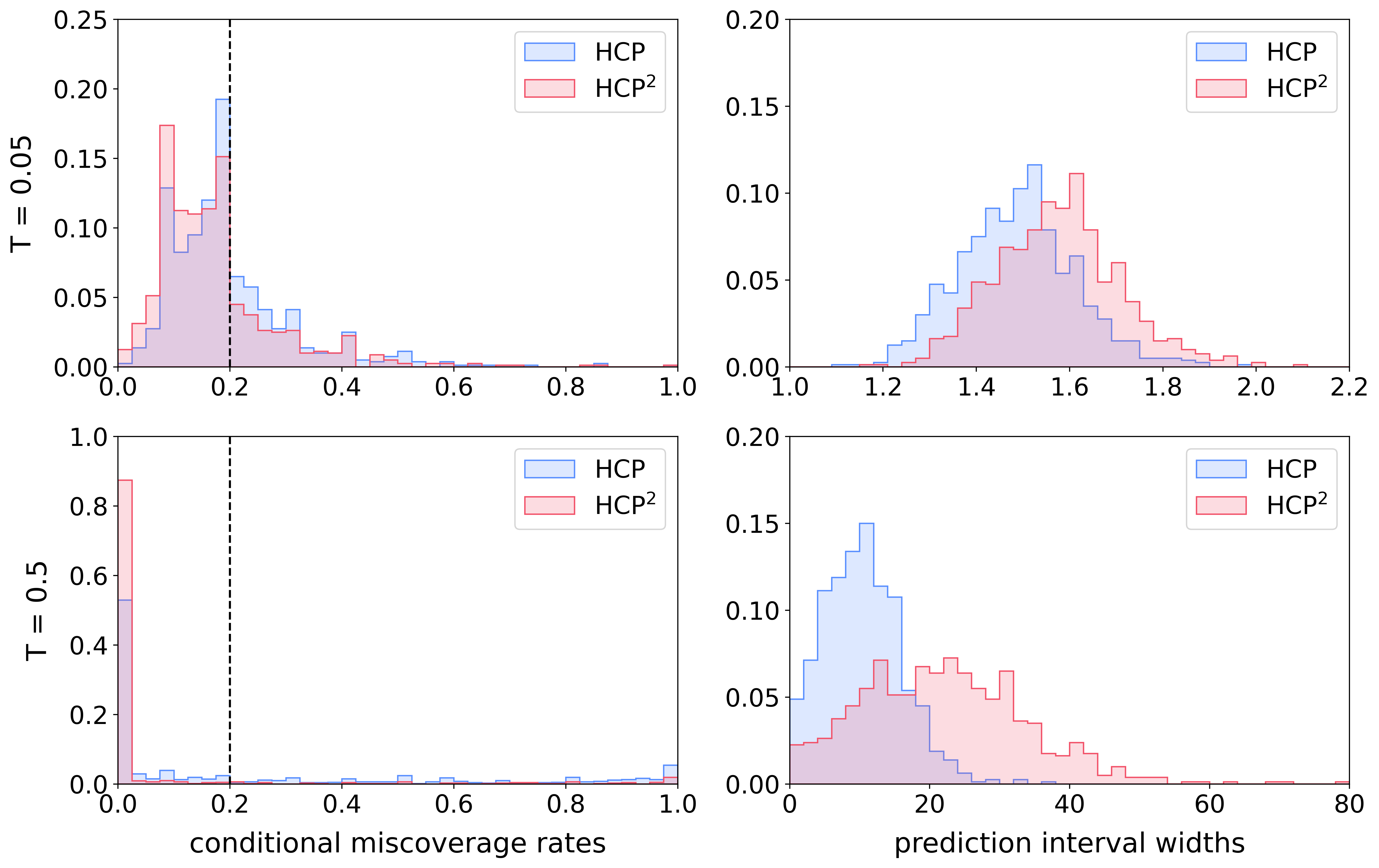
We run 500 independent trials of the simulation. For each trial, each of the two settings, and each method (HCP and HCP2), after generating the training data and the test point we construct a prediction set , and then compute the conditional miscoverage rate (which can be computed exactly, since the distribution of is known by construction) and the width of the prediction set .
The results for the residual score are shown in Figure LABEL:fig:sim_hist_residual. We see that, for Setting 1 (constant variance), where this score is a good match for the shape of the conditional distribution of , both HCP and HCP2 show conditional miscoverage rates that cluster closely around the target level , and consequently, the prediction interval width are similar for the two methods. For Setting 2 (nonconstant variance), on the other hand, this score is a poor match for the distribution, and while HCP achieves an average coverage of 80%, the distribution of has extremely large variance. It is clear that HCP does not satisfy any sort of conditional coverage or second-moment coverage property, and consequently HCP2 is forced to produce substantially wider prediction intervals, illustrating the tradeoff between width of the interval and the coverage properties it achieves.
In contrast, the results for the rescaled residual score are shown in Figure LABEL:fig:sim_hist_standardized. This choice of score is a good match for the data distribution in both Setting 1 and Setting 2, since it accommodates nonconstant variance. Consequently, for both HCP and HCP2, we see that the empirical distribution of clusters around the target level , and the two methods produce similar prediction interval widths. Thus we see that, when the score function is chosen well, the stronger coverage guarantee offered by HCP2 is essentially “free” since we can achieve it without substantially increasing the width of the prediction intervals.
4 Application to a dynamical system dataset
Our study is inspired by the generation of ensembles of climate forecasts created by running a simulator over a collection of perturbed initial conditions. These so-called “initial condition ensembles” help decision-makers account for uncertainties in forecasts when developing climate change mitigation and response plans (Mankin et al., 2020). Similar ensembles are used for weather forecasting; for instance, the European Centre for Medium-Range Weather Forecasts (ECMWF) notes:
An ensemble weather forecast is a set of forecasts that present the range of future weather possibilities. Multiple simulations are run, each with a slight variation of its initial conditions and with slightly perturbed weather models. These variations represent the inevitable uncertainty in the initial conditions and approximations in the models. (European Centre for Medium-Range Weather Forecasts, 2023)
Overview of experiment.
For this experiment,999Code to reproduce this experiment is available at https://github.com/rebeccawillett/Distribution-free-inference-with-hierarchical-data. our task will be to predict the future state of the system, looking ahead from current time to future time . We will consider two different choices of for defining both an easier task (near-future prediction with a low value of ) and a harder task (prediction farther into the future, with a higher value of ). We will see that, while HCP provides marginal coverage (as guaranteed by the theory) for both tasks, second-moment coverage only appears to hold empirically for the easier task; consequently, HCP2 is able to return intervals that are only barely wider for the easier near-future prediction task, but for the harder task must return substantially wider intervals in order to achieve a second-moment coverage guarantee.
Generating the data.
In the context of this paper, we seek to take an initial condition and generate a prediction interval that contains all ensemble forecasts with high probability. Motivated by this setting, we apply HCP and HCP2 to a dynamical system dataset generated from the Lorenz 96 (L96) model. Developed by Lorenz (1996), the L96 system is a prototype model for studying prediction and filtering of dynamical systems in climate science. The model is a system of coupled ordinary equations and defined as follows:
| (18) |
where denotes the state of the system at different locations . In order for the system to be well-defined at the boundaries, we define , , ; this ensures that the system is cyclic over the locations. The value denotes the external forcing, i.e., an effect of external factors; we use , which corresponds to strong chaotic turbulence (Majda et al., 2005).
To specify our workflow, we define a function that runs the L96 system as defined in (18) for a time duration (more precisely, this function implements the Runge–Kutta approximation with time step , (Bank et al., 1987; SciPy.org, )). Thus, given starting conditions , the value of the system at time , , is (approximately) given by
To generate data, we do the following: taking as the number of independent groups of observations, independently for each ,
-
•
The feature vector is , with dimension , which defines the initial conditions of the system.
-
•
Setting , for each , start the L96 system initialized at a perturbation of ,
with the scale of the noise set as . We then run the L96 system (18) up until time to define the response:
i.e., the value of the system at the final time , at its first location, .
The feature vectors , i.e., the initial conditions, are themselves generated using the L96 system as well, in order to provide more meaningful or realistic starting conditions: independently for each ,
i.e., is the output of the L96 system run for time duration (where we take ) when initialized with Gaussian noise.
We consider two different choices of , to define two different prediction tasks: a near-future prediction task, with , and a more distant-future prediction task, with . For each of the two tasks, we generate training, calibration, and test sets as described above, where each data set has and . We run a neural network model on the training data set to produce estimators and of the conditional mean and conditional standard deviation of given . Using the calibration data, we then implement the HCP and HCP2 methods, with score function .
Results.
We evaluate the performance of the two procedures with the test data. The results are summarized in Table 1 and Figure 2.
| Mean width | ||||
|---|---|---|---|---|
| T = 0.05 | HCP | 0.2006 (0.0041) | 0.0546 (0.0029) | 1.4875 (0.0044) |
| HCP2 | 0.1748 (0.0039) | 0.0437 (0.0026) | 1.5753 (0.0047) | |
| T = 0.5 | HCP | 0.2313 (0.0119) | 0.1701 (0.0110) | 10.4259 (0.1957) |
| HCP2 | 0.0628 (0.0073) | 0.0478 (0.0066) | 22.0395 (0.4138) |
The results show that HCP and HCP2 provide prediction sets that satisfy their respective target guarantees. Since the dynamical system is chaotic, making accurate predictions become harder for larger . For the task of predicting the relatively near future (), the two procedures provide similar prediction sets. In particular, we see that HCP already achieves second-moment miscoverage near the target level ; consequently, HCP2 is able to return a similar prediction interval as HCP, without being substantially more conservative. In contrast, for the task of predicting the far future (), while HCP successfully bounds the marginal miscoverage rate with relatively narrow prediction intervals, it fails to achieve good conditional miscoverage control (indeed, HCP shows a high second-moment miscoverage rate—nearly as large as , i.e., the worst-case scenario as described in Section 3.3.1). As a result the HCP2 method needs to be much more conservative (wider prediction sets than HCP) in order to reduce second-moment miscoverage to the allowed level .
5 Discussion
In this work, we examine the problem of distribution-free inference for data sampled under a hierarchical structure, and propose hierarchical conformal prediction (HCP) to extend the conformal prediction framework to this setting. We also examine the special case of repeated measurements (multiple draws of the response for each sampled feature vector ), and develop the HCP2 method to achieve a stronger second-moment coverage guarantee, moving towards conditional coverage in this setting.
These results raise a number of open questions. In many statistical applications, the hierarchical structure of the sampling scheme is (at least partially) controlled by the analyst designing the study. In particular, this means that the analyst can choose between, say, a large number of independent groups with a small number of measurements within each group, or conversely a small number of groups with large numbers of repeats. Characterizing the pros and cons of this tradeoff is an important question to determine how study design affects inference in this distribution-free setting.
Our results show that having even a small amount of repeated measurements can significantly expand the realm of what distribution-free inference can do (relatedly, recent work by Lee and Barber (2021) examines a similar phenomenon when the distribution of is discrete). This raises a more general question: what reasonable additions can we make to the setting so that a more useful inference is possible in a distribution-free manner? We aim to explore this type of problem in our future work.
Acknowledgements
Y.L., R.F.B., and R.W. were partially supported by the National Science Foundation via grant DMS-2023109. Y.L. was additionally supported by National Institutes of Health via grant R01AG065276-01. R.F.B. was additionally supported by the Office of Naval Research via grant N00014-20-1-2337. R.W. was additionally supported the National Science Foundation via grant DMS-1930049 and by the Department of Energy via grant DE-AC02-06CH113575. The authors thank John Duchi for catching an error in an earlier draft of this paper.
References
- Bank et al. [1987] R Bank, RL Graham, J Stoer, and R Varga. Springer series in 8. 1987.
- Barber [2020] Rina Foygel Barber. Is distribution-free inference possible for binary regression? Electronic Journal of Statistics, 14(2):3487–3524, 2020.
- Barber et al. [2021a] Rina Foygel Barber, Emmanuel J Candes, Aaditya Ramdas, and Ryan J Tibshirani. The limits of distribution-free conditional predictive inference. Information and Inference: A Journal of the IMA, 10(2):455–482, 2021a.
- Barber et al. [2021b] Rina Foygel Barber, Emmanuel J Candes, Aaditya Ramdas, and Ryan J Tibshirani. Predictive inference with the jackknife+. The Annals of Statistics, 49(1):486–507, 2021b.
- Barber et al. [2022] Rina Foygel Barber, Emmanuel J Candes, Aaditya Ramdas, and Ryan J Tibshirani. Conformal prediction beyond exchangeability. arXiv preprint arXiv:2202.13415, 2022.
- Cheng et al. [2022] Chen Cheng, Hilal Asi, and John Duchi. How many labelers do you have? a closer look at gold-standard labels. arXiv preprint arXiv:2206.12041, 2022.
- Chernozhukov et al. [2021] Victor Chernozhukov, Kaspar Wüthrich, and Yinchu Zhu. Distributional conformal prediction. Proceedings of the National Academy of Sciences, 118(48):e2107794118, 2021.
- Dunn et al. [2022] Robin Dunn, Larry Wasserman, and Aaditya Ramdas. Distribution-free prediction sets for two-layer hierarchical models. Journal of the American Statistical Association, pages 1–12, 2022.
- European Centre for Medium-Range Weather Forecasts [2023] European Centre for Medium-Range Weather Forecasts. Fact sheet: Ensemble weather forecasting, 2023. https://www.ecmwf.int/en/about/media-centre/focus/2017/fact-sheet-ensemble-weather-forecasting, Retrieved Oct. 13, 2023.
- Harrison [2012] Matthew T Harrison. Conservative hypothesis tests and confidence intervals using importance sampling. Biometrika, 99(1):57–69, 2012.
- Izbicki et al. [2019] Rafael Izbicki, Gilson T Shimizu, and Rafael B Stern. Flexible distribution-free conditional predictive bands using density estimators. arXiv preprint arXiv:1910.05575, 2019.
- Lee and Barber [2021] Yonghoon Lee and Rina Barber. Distribution-free inference for regression: discrete, continuous, and in between. Advances in Neural Information Processing Systems, 34, 2021.
- Lei and Wasserman [2014] Jing Lei and Larry Wasserman. Distribution-free prediction bands for non-parametric regression. Journal of the Royal Statistical Society: Series B: Statistical Methodology, pages 71–96, 2014.
- Lei et al. [2015] Jing Lei, Alessandro Rinaldo, and Larry Wasserman. A conformal prediction approach to explore functional data. Annals of Mathematics and Artificial Intelligence, 74:29–43, 2015.
- Lei et al. [2018] Jing Lei, Max G’Sell, Alessandro Rinaldo, Ryan J Tibshirani, and Larry Wasserman. Distribution-free predictive inference for regression. Journal of the American Statistical Association, 113(523):1094–1111, 2018.
- Lorenz [1996] Edward N Lorenz. Predictability: A problem partly solved. In Proc. Seminar on predictability, volume 1. Reading, 1996.
- Majda et al. [2005] Andrew Majda, Rafail V Abramov, and Marcus J Grote. Information theory and stochastics for multiscale nonlinear systems, volume 25. American Mathematical Soc., 2005.
- Mankin et al. [2020] Justin S Mankin, Flavio Lehner, Sloan Coats, and Karen A McKinnon. The value of initial condition large ensembles to robust adaptation decision-making. Earth’s Future, 8(10):e2012EF001610, 2020.
- Medarametla and Candès [2021] Dhruv Medarametla and Emmanuel Candès. Distribution-free conditional median inference. Electronic Journal of Statistics, 15(2):4625–4658, 2021.
- Papadopoulos et al. [2002] Harris Papadopoulos, Kostas Proedrou, Volodya Vovk, and Alex Gammerman. Inductive confidence machines for regression. In European Conference on Machine Learning, pages 345–356. Springer, 2002.
- Podkopaev and Ramdas [2021] Aleksandr Podkopaev and Aaditya Ramdas. Distribution-free uncertainty quantification for classification under label shift. In Uncertainty in Artificial Intelligence, pages 844–853. PMLR, 2021.
- Romano et al. [2019] Yaniv Romano, Evan Patterson, and Emmanuel Candes. Conformalized quantile regression. Advances in neural information processing systems, 32, 2019.
- [23] SciPy.org. https://docs.scipy.org/doc/scipy/reference/generated/scipy.integrate.solve_ivp.html#r179348322575-13.
- Tibshirani et al. [2019] Ryan J Tibshirani, Rina Foygel Barber, Emmanuel Candes, and Aaditya Ramdas. Conformal prediction under covariate shift. Advances in neural information processing systems, 32, 2019.
- Vovk [2012] Vladimir Vovk. Conditional validity of inductive conformal predictors. In Asian conference on machine learning, pages 475–490. PMLR, 2012.
- Vovk [2015] Vladimir Vovk. Cross-conformal predictors. Annals of Mathematics and Artificial Intelligence, 74:9–28, 2015.
- Vovk and Wang [2020] Vladimir Vovk and Ruodu Wang. Combining p-values via averaging. Biometrika, 107(4):791–808, 2020.
- Vovk et al. [2005] Vladimir Vovk, Alexander Gammerman, and Glenn Shafer. Algorithmic learning in a random world. Springer Science & Business Media, 2005.
- Vovk et al. [2018] Vladimir Vovk, Ilia Nouretdinov, Valery Manokhin, and Alexander Gammerman. Cross-conformal predictive distributions. In Conformal and Probabilistic Prediction and Applications, pages 37–51. PMLR, 2018.
- Xu and Xie [2021] Chen Xu and Yao Xie. Conformal prediction interval for dynamic time-series. In International Conference on Machine Learning, pages 11559–11569. PMLR, 2021.
Appendix A Extending HCP to full conformal and jackknife+
In Sections 2 and 3, we introduced methods that extend split conformal prediction to the setting of hierarchical exchangeability, constructing prediction sets with the marginal coverage guarantee (via the HCP method) and the stronger second-moment coverage guarantee (via the HCP2 method). Similar ideas can be applied to derive extensions of other methods—specifically, full conformal prediction [Vovk et al., 2005] and jackknife+ [Barber et al., 2021b]—to the hierarchical data setting, which allows us to avoid the statistical cost of data splitting.
A.1 Extending full conformal prediction
A.1.1 Background: full conformal prediction
In the setting of exchangeable data (without a hierarchical structure), the full conformal prediction method [Vovk et al., 2005] allows us to use the entire training data set for constructing the score function, rather than splitting the data as in split conformal. Specifically, the method begins with an algorithm , which inputs a data set of size and returns a fitted score function ; is assumed to be symmetric in its input arguments, i.e., permuting the input data points does not affect .101010The framework also allows for a randomized algorithm , in which case the symmetry condition is required to hold in a distributional sense. Define
the fitted score function obtained if were the test point. The prediction set is then given by
For exchangeable training and test data, this method offers marginal coverage at level [Vovk et al., 2005].
A.1.2 Hierarchical full conformal prediction
We now define a version of HCP that extends the full conformal method to the hierarchical framework. We now begin with an algorithm , again assumed to be symmetric—but now the symmetry follows a hierarchical structure: we assume that, for any , first, it holds that
for all , and, second,
for all and all . We refer to any such algorithm as hierarchically symmetric. (For example, if simply discards the group information and runs a symmetric procedure on the data points , then the hierarchical symmetry property follows immediately—in this sense, then, requiring hierarchical symmetry is strictly weaker than the usual symmetry condition.)
Next, define
to be the fitted score function obtained if we were to observe an entire group of test observations , and let
where denotes the projection to the first component (i.e., if , then ). Let
| (19) |
where .
Since is a space of vectors of arbitrary lengths, this prediction set has heavier computational cost than the full conformal method in standard settings, which already is known to have a high computational cost. It is therefore unlikely to be useful in practical settings; this extension is therefore primarily of theoretical interest, and is intended only to demonstrate that the hierarchical exchangeability framework can be combined with full conformal as well as with split conformal.
Our first theoretical result shows that this method provides a marginal coverage guarantee in the hierarchical data setting.
Theorem 3.
Suppose that satisfies the hierarchical exchangeability property (Definition 1), and let . Given a hierarchically symmetric algorithm , the prediction set defined above satisfies
Similarly, we can achieve a bound for the second-moment coverage via full-conformal framework. We extend HCP2 to this setting. Define , and let
and then again define as in (19). Again, as above, this construction is computationally extremely expensive and is therefore primarily of theoretical interest.
Theorem 4.
A.2 Extending jackknife+
A.2.1 Background: jackknife+
The jackknife+ [Barber et al., 2021b] (closely related to cross-conformal prediction [Vovk, 2015, Vovk et al., 2018]) offers a leave-one-out approach to the problem of distribution-free predictive inference. Like full conformal, the jackknife+ method provides a prediction set without the loss of accuracy incurred by data splitting. The computational cost of jackknife+ is higher than for split conformal (requiring fitting many leave-one-group-out models), but substantially lower than full conformal.
Rather than working with an arbitrary score function, jackknife+ works specifically with the residual score (i.e., for some fitted model ), in the setting . Let , which inputs a data set of size and returns a fitted regression function ; as for full conformal, is assumed to be symmetric in its input arguments. Let
be the th leave-one-out model, and compute the th leave-one-out residual as
Then the jackknife+ prediction interval is given by
where for a distribution on , (compare to the usual definition of quantile, where we take the infimum rather than the supremum). For exchangeable training and test data, the jackknife+ offers marginal coverage at level (here the factor of 2 is unavoidable, unless we make additional assumptions) [Barber et al., 2021b].
A.2.2 Hierarchical jackknife+
Next, we extend jackknife+ to the hierarchical setting. (HCP can also be extended to cross-conformal prediction [Vovk, 2015, Vovk et al., 2018] in a similar way, but we omit the details here.) While computationally more expensive than split conformal based methods, the hierarchical jackknife+ can nonetheless be viewed as a practical alternative to the computationally infeasible full conformal based method.
To define the hierarchical jackknife+ method, we begin with an algorithm , which we again assume to be hierarchically symmetric, as for the case of full conformal. For each , define the leave-one-group-out model,
and define the corresponding residuals for the th group,
for each . The hierarchical jackknife+ prediction interval is then given by
| (20) |
Our first theoretical result shows that this method provides a marginal coverage guarantee in the hierarchical data setting.
Theorem 5.
We can also obtain a second-moment coverage bound by extending HCP2 to the jackknife+. Define
| (21) |
Theorem 6.
Appendix B Comparing HCP2 versus a trivial solution
In Section 3.3.1, we discussed a possible trivial solution to the problem of second-moment coverage: simply run a method that guarantees marginal coverage, at level in place of . Here we illustrate that this trivial solution is, as expected, highly impractical because it inevitably provides extremely wide prediction intervals; we compare to HCP2 which is able to keep intervals at roughly the same width as a marginal-coverage method, in settings where the score function is chosen well.
To illustrate this, we rerun the simulations of Section 3.4, adding a third method: HCP run with in place of . All other details of the data and implementation are exactly the same as in Section 3.4.111111Code to reproduce this simulation is available at https://github.com/rebeccawillett/Distribution-free-inference-with-hierarchical-data.
As expected, we see that, for the three cases where the score function is a good match to the data distribution (namely, the residual score for Setting 1, or the rescaled residual score for Setting 1 and for Setting 2), HCP2 provides intervals that are similar in width to HCP, while running the trivial solution (HCP with in place of ) leads to extremely wide intervals. On the other hand, for the fourth case (the residual score for Setting 2), HCP2 shows poor performance, but is still noticeably better than simply running the trivial solution (HCP with in place of ); the trivial solution is still overly conservative, although less so here than in the other three cases.
Appendix C Proofs
C.1 Proof of Theorem 1
As described in Section 1.1, we can define , so that the combined data set satisfies hierarchical exchangeability (Definition 1), where for each and for each .
From this point on, we perform all calculations conditional on the training data , so that we can treat the score function as fixed. Note that, conditional on the training data , the remaining data (i.e., the calibration and test groups) again satisfy hierarchical exchangeability (Definition 1).
A new quantile function.
First, define a function as
the empirical quantile of a given data set reweighted according to group size (to give equal weight to each group regardless of length). By definition of as a weighted quantile, it holds deterministically that
| (22) |
(see, e.g., Harrison [2012, Lemma A1]), and furthermore, if for any , then
| (23) |
where this last step holds since the condition on the scores ensures that the weighted distribution places mass at most on any value.
Next, we examine the invariance properties of this function . First, for any , we can verify that
| (24) |
Next, for any consider a permutation , and let be the corresponding permutation of . We can see from the definition that
| (25) |
Applying hierarchical exchangeability.
Recall the definition of hierarchical exchangeability (Definition 1): by the second part of the definition, for any permutation , we have
conditional on both and on . Then, conditional on and , for any ,
where the second step holds by (25). In particular, by taking any with ,
for each . After taking an average over all , and then marginalizing over ,
Coverage guarantee: lower bound.
Now we need to relate the function to the coverage properties of the HCP method. Recalling the definition (6) of the HCP prediction interval, we can see that
and so
Therefore, combining with the work above,
Coverage guarantee: upper bound.
Finally, we derive the upper bound on coverage, in the case that for all , almost surely. First, we can observe that
where . Therefore, from the calculations above (applied with in place of ),
C.2 Proof of Theorem 2
The proof largely follows the same structure as the proof of Theorem 1.
First, draw from the distribution of conditional on the event , and draw i.i.d. from the distribution of at . Condition also on . Then, conditional on and also on the training data , we see that
satisfies hierarchical exchangeability (Definition 1).
A new quantile function.
Next, define , and define a function as
By definition of this weighted quantile, it holds deterministically that
| (26) |
(see, e.g., Harrison [2012, Lemma A1]).
Next, we examine invariance properties of this function . Similarly to the proof of Theorem 1, for any , we see that the value of is unchanged if we permute groups, or if we permute data points within any group.
Applying hierarchical exchangeability.
Coverage guarantee.
Now we need to relate the function to the coverage properties of the HCP2 method. For each , we have if and only if
by definition of the method. Deterministically, it holds that this quantile on the right hand side is , and so,
In particular,
where the last step holds by the work above. Equivalently,
Next, since are i.i.d. draws from the distribution at (and are independent of the training and calibration data, by the hierarchical i.i.d. model),
Combining with the above, and marginalizing, we have
where the last step holds by definition of . Recalling that by construction, this completes the proof of the upper bound on .
The upper bound.
In the case that for all , almost surely, proving that
follows from an argument that is very similar to the proof of the analogous result in Theorem 1, so we omit the details. Finally, we can verify that
by using the fact that .
C.3 Proof of Theorem 5
The proof extends the idea of the proof for the original jackknife+ [Barber et al., 2021b]. Similarly to the proof for the split conformal-based methods we look into the coverage for . For each , let be the estimator from the expanded data set after excluding the -th and -th groups of observations, and define by
for . Next, define
and note that for any , we must have . Define also
Write to denote the array of all ’s:
Finally, define the set by
and let
To bound , we have
which proves .
Next, since satisfies hierarchical exchangeability (Definition 1), by a similar argument as in the proof of Theorem 1, we have
for all , where is any positive integer with , and
for all . It follows that
where the last inequality holds since we have shown that holds deterministically.
Now suppose . This implies that either
or
From the definition of and , we then have
or
In either case, we have
Hence, we have shown that implies , and so
C.4 Proof of Theorem 6
For with , , and , define as in the proof of Theorem 5, and then define
and
and note that for any , we must have . Next, let
where
and
which we assume to be nonzero. Let
We then calculate
which proves .
Next, by an analogous argument as in the proof of Theorem 5, the hierarchical exchangeability of the data implies that
where the last step holds by our deterministic bound on calculated above. Our next step is to verify that
| (27) |
To see this, by definition of we see that, for each , implies that
Summing over , then, we have
This verifies (27), and so we have
To complete the proof, we calculate
where the last two steps hold by definition of and of . Therefore,