Distributed Speculative Inference of Large Language Models is Provably Faster
Abstract
Accelerating the inference of large language models (LLMs) is an important challenge in artificial intelligence. This paper introduces distributed speculative inference (DSI), a novel distributed inference algorithm that is provably faster than speculative inference (SI) (Leviathan et al., 2023; Chen et al., 2023; Miao et al., 2023) and traditional autoregressive inference (non-SI). Like other SI algorithms, DSI works on frozen LLMs, requiring no training or architectural modifications, and it preserves the target distribution. Prior studies on SI have demonstrated empirical speedups (compared to non-SI) but require fast and accurate drafters, which are often unavailable in practice. We identify a gap where SI can be slower than non-SI given slower or less accurate drafters. We close this gap by proving that DSI is faster than both SI and non-SI—given any drafters. DSI introduces a novel type of task parallelism called Speculation Parallelism (SP), which orchestrates target and drafter instances to overlap in time, creating a new foundational tradeoff between computational resources and latency. DSI is not only faster than SI but also supports LLMs that cannot be accelerated with SI. Our simulations show speedups of off-the-shelf LLMs in realistic single-node settings where DSI is 1.29-1.92x faster than SI. 111All the code is open-source under Apache-2.0 license.
1 Introduction
Generative LLMs, such as GPT-4 (OpenAI, 2023), have demonstrated unprecedented results in various applications (Andreas, 2022; Li et al., 2023; Bubeck et al., 2023; Wei et al., 2022). Despite their potential, the inference latency of LLMs presents a significant challenge and a bottleneck for adoption in real-time applications. For example, in algorithmic trading, the model needs to make rapid predictions to execute trades in milliseconds (Tan et al., 2024; Zhang et al., 2023), and in autonomous driving, the model must act quickly to ensure the vehicle’s reliability (Yang et al., 2024). Real-time applications often prioritize low latency over other objectives, and in particular are willing to trade off more computational resources for faster inference. With the growing availability of hardware and decrease in its costs, finding how to effectively utilize more computing power for faster inference becomes increasingly important.
Given their usefulness, speeding up the inference of LLMs is an important area of research. Existing efforts to reduce the inference latency can be classified into two main categories by their approach to hardware utilization. The first category focuses on making LLMs use less computing resources or better utilize the same resources. This includes post-training compression through pruning (e.g., (Frantar and Alistarh, 2023; Sun et al., 2024a; Ma et al., 2023)), knowledge distillation (e.g., Hinton et al. (2015); Gu et al. (2024)), quantization (e.g., (Hubara et al., 2018; Frantar et al., 2023; Lin et al., 2024; Yao et al., 2024; Dettmers et al., 2022)), low-rank factorization (e.g., (Hsu et al., 2022; Xu et al., 2023)), early existing (e.g., (Schuster et al., 2022; Kim et al., 2023; Elbayad et al., 2020; Bapna et al., 2020; Schuster et al., 2021)), and alternative architectures (e.g., (Cai et al., 2024; Li et al., 2024; Zhang et al., 2024b, a; Xiao et al., 2024; Gu and Dao, 2023)). While these solutions are useful in practice, they often require modifications to the model architecture, changes to the training procedure and re-training of the models, without guaranteeing identical outputs. Despite reducing the inference time, these methods often have a significant drawback of degrading the output quality. There are also solutions that preserve the output quality, such as kernel optimizations (Dao et al., 2022; Dao, 2024), but they highly depend on the hardware and therefore are not always available or even feasible. The second category focuses on accelerating the inference by using more computing power. It includes data parallelism (DP) and model parallelism (MP) methods of different types, such as pipeline parallelism (PP), tensor parallelism (TP) (Narayanan et al., 2021), and context parallelism (CP) (Harper et al., 2019). Such partitioning over multiple processors can speed up memory-bounded inference setups, for example, by avoiding memory offloading. They are often effective in increasing the inference throughput and supporting larger context length. However, the typical LLM architectures necessitate autoregressive inference. Such inference is inherently sequential with only limited (if any) MP opportunities, depending on the LLM architecture. Since the portion of the inference that could be parallelized is small (if any) in typical LLMs, the potential speedup of MP methods is limited, by Amdahl’s law. Hence, while DP methods can increase the inference throughput, they remain inherently sequential. Furthermore, as the parallelisms above shard over more processors, the communication overhead increases, which can lead to diminishing returns, limiting the number of processors they can effectively utilize.
A recent line of work (Stern et al., 2018) for accelerating the inference of LLMs is based on speculative inference. The idea is to use speculative execution (Burton, 1985; Hennessy and Patterson, 2012) to predict possible continuations of the input prompt using faster drafter LLMs that approximate the target LLM, then verify the correctness of the predicted continuations simultaneously by utilizing data parallelism capabilities of CUDA-based processors known as batching. They provided empirical evidence that their proposed draft-then-verify approach speeds up the inference. Since the introduction of speculative inference (SI) by Stern et al. (2018), various papers (Leviathan et al., 2023; Chen et al., 2023) have improved this method by introducing novel lossless methods to verify the correctness of token sequences that were generated by the drafter LLMs. Empirically, these approaches lead to speedups in practical use cases, such as 2-3x speedups in decoding LLMs of 11B and 70B parameters in some settings. Following this line of work, Miao et al. (2023) extended the verification algorithm of Leviathan et al. (2023); Chen et al. (2023) and showed that their method increases the probability of accepting draft tokens, and proved its losslessness. Following the success of this approach, research in this area has expanded in various directions (Mamou et al., 2024; Li et al., 2024; Cai et al., 2024; Sun et al., 2024b; Zhou et al., 2024; Liu et al., 2023; Joao Gante, 2023). Most recently, Chen et al. (2024) showed that lossless SI can effectively reduce the inference latency while increasing its throughput, in the multi-user setting. The effectiveness of SI algorithms comes from their ability to reduce the number of target forwards by using GPU batching such that a single target forward is sufficient for generating more than one token. However, existing SI methods implement a sequential process, repeatedly drafting and verifying. They never draft more tokens before the previous verification ends. This limitation implies that SI speeds up the inference if and only if the drafter is sufficiently fast and accurate, as studied in this paper. In cases where the drafter is too slow or inaccurate, SI is slower than non-SI.
Contributions. Our proposed method, distributed speculative inference (DSI), introduces a novel task parallelism for SI, named speculation parallelism (SP), to make the blocking verifications of SI non-blocking. DSI leverages SP to hide the verification latency of iterations without a draft rejection. Unlike SI, which can run on a single GPU, DSI requires two or more GPUs. DSI is useful in practice because it works given an arbitrary number of GPUs () by adjusting its lookahead hyperparameter. Provably, DSI is faster than SI in expectation and always as fast or faster than non-SI (§3.2). DSI can accelerate inference even when drafters slow down SI compared to non-SI, thus enabling the acceleration of more off-the-shelf LLMs. Empirically, DSI on a single node with up to eight GPUs is significantly faster than both SI and non-SI (§4).
2 Preliminaries
We begin by describing autoregressive language models, next-token prediction, speculative inference and how to measure latency.
Autoregressive language models (LMs) are deterministic, real-valued multivariate functions. An input to an LM is a sequence of vectors of dimension . We call these vectors tokens, and the sequence a prompt. LMs output a real-valued vector of dimension , also known as the logits. Since prompts may vary in length, we simplify the notation of the forward pass as follows: .
Self-Attention LMs are LMs with a pre-defined context length (Vaswani et al., 2017). Hence, we represent the forward pass of such LMs in the following manner: . For example, GPT-2 and GPT-3 are Transformers with , and context lengths and , respectively (Radford et al., 2019; Brown et al., 2020). In this paper, all LMs are Self-Attention ones with pre-set (frozen) parameters.
We extend the prompt notation such that prompts can have length . Self-Attention LMs handle prompts of length by starting the input sequence with a prefix of tokens, followed by the given tokens. LMs ignore the prefix, either by zeroing (masking) the Attention parts corresponding to the prefix or by left-padding with dedicated tokens. In this paper, prompts of length are the non-masked, non-padded suffix of the input sequence of length .
Generating the next token is the primary application of autoregressive LMs. This process consists of two steps: computing the forward pass of the LM and then selecting the next token based on the output. The selection can be deterministic or non-deterministic. Non-deterministic selection procedures apply the softmax function after the forward pass of LMs and sample from the resulting probability vector:
| (1) |
For convenience, we denote the output probability vector by :
| (2) |
where is the concatenation of the vectors and and . For deterministic selection procedures, composing monotonic functions, such as softmax, is usually unnecessary. For example, the most likely next token is the of both the logits and the output of the softmax. Still, for convenience, we assume that LMs always output probability vectors. The sampling process in (2) is either deterministic (i.e., is a token with maximal probability) or random (achieved by randomly selecting from the distribution ).
Speculative Inference (SI) is an approach for accelerating the inference of a target LM (e.g., a member of the GPT series) . Such methods use faster LMs that approximate the target model in order to reduce the total inference time. For example, Leviathan et al. (2023); Chen et al. (2023) may reduce the amount of time to infer a target model on a given prompt by using batching as follows. The inference starts by drafting tokens for using a faster drafter model . Then, the algorithm sends the prompts altogether as one input batch to the target model . The idea is to take advantage of the data parallelism that modern GPUs offer to compute the logits corresponding to the prompts in parallel, hence faster than computing these individual logits sequentially. Given the logits, the algorithm generates tokens without additional forward passes. By repeating this process, the algorithm can generate tokens.
Straightforward algorithms of speculative inference are typically lossless in expectation, i.e., they generate tokens from the same distributions as the target would generate without speculation. Naive algorithms of speculation guarantee returning the same tokens as the target (Joao Gante, 2023; Spector and Re, 2023). More sophisticated algorithms of speculation might generate different tokens, but their generated tokens follow the distribution of the target (Leviathan et al., 2023; Chen et al., 2023).
To implement distributed algorithms for speculative inference, we use multiple processors or servers, which are hardware components capable of executing threads. Processors can compute forward passes and sample tokens from the output probability vectors and we assume that threads can run in parallel. When using DSI we will run sequences of drafter models , where the first model takes and returns some token , the second takes as a prompt and returns , and so on. As such, in order to denote that a given thread is computing the output of on a sequence , we denote , where . When a thread computes an LM, we denote the output probability vector by . If samples a new token from , we denote this token by . For example, thread implementing (2) above will have
Once a thread finishes sampling a new token, the thread outputs the concatenation of and . Following the example in (2), we have
A new thread that was initiated by is denoted by , where is the concatenation of and . The set of all the threads that originate from is . We assume that terminating a concurrent thread terminates all the threads that originate from it.
Time in this paper is the wall time. We measure the time that passes from the initiation of a task until its termination. A task is a nonempty set of threads, denoted by . Its time is
When a task consists of a single thread, we omit the curly brackets, namely,
Note that two threads, denoted by and , may run concurrently and overlap in time. Hence, it is possible that . However, if and do not overlap in time, then .
3 Distributed Speculative Inference
This section lays out a theoretically sound framework to parallelize SI (Leviathan et al., 2023; Chen et al., 2023; Miao et al., 2023). The naive version of our method assumes access to a sufficiently large number of processors so that threads never have to wait. Later, we discuss implementing our method with a fixed number of processors.
Before presenting our algorithm, we first discuss the limitations of existing SI methods. SI reduces target forwards whenever a draft token is accepted. With an accurate and fast drafter, SI can significantly cut the number of target forwards, potentially speeding up the inference compared to non-SI. For instance, if on average one draft is accepted per iteration, the number of target forwards drops to half since the average target forward generates two tokens. As long as the total drafting latency is less than the saved latency from reduced target forwards, SI offers a speedup over non-SI. The main limitation of existing SI methods is their sequential nature. Each SI iteration requires a target forward, and the next iteration only begins after the current one is completed. However, we observe that the verification of each SI iteration is not inherently sequential and could be parallelized.
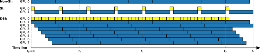
Previous works on SI exemplified speedups using drafters that run within 1-5% of the time (compared to the target LLM), and iterations of 2-5 draft tokens (namely, ). We can calculate the maximum speedup of our proposed method compared to SI by Amdahl’s law, as follows. Assume the drafter is perfectly accurate. In that case, our method hides all the verification latency such that the overall end-to-end latency remains only the drafting latency. For drafters of 1-5% latency and , our proposed parallelization leads to a theoretical speedup of 4x-50x compared to SI. Figure 1 and Table 1 illustrate potential speedups compared to SI and non-SI, given a drafter of 14% latency.
| worst case: non-SI | 0 | 2 | 4 | 8 | 9 |
| worst case: SI | 0 | 1 | 4 | 7 | 8 |
| worst case: DSI | 0 | 2 | 4 | 8 | 9 |
| best case: non-SI | 0 | 2 | 4 | 8 | 9 |
| best case: SI | 0 | 2 | 8 | 14 | 16 |
| best case: DSI | 0 | 8 | 26 | 50 | 58 |
3.1 Method Overview
Consider the task of computing output tokens autoregressively from a target model given a prompt . We have a set of faster drafter models, , that are all faster than (as defined in Assumption 2). Our goal is to compute for all . To achieve this, we initiate threads, (line 2). Each thread, denoted as , is responsible for computing . Once a thread, , finishes computation, we instantiate new threads, , to calculate for all . In general, once we compute , we initiate new threads, , to compute for all . This is captured in lines 4 and 6.
Once completes its computation and provides the correct value of the first output token , we can verify which other threads, , have accurately computed . Any thread where is immediately terminated along with its descendant processes. For each that correctly computed , we continue with computing for all . However, since all threads are computing the same set of tokens, we terminate all but the one corresponding to the smallest value of that satisfies . In essence, serves as a verifier, identifying drafters that miscalculated the initial part of the autoregressive computation. Once we retain one valid , we relabel as the new verifier thread. We know that since returned the correct token and , the output of must be correct. When that thread finishes, among the remaining threads, , we terminate those that miscalculated and keep only the one with , whose index is minimal. We continue this process until the output is obtained from the last verifier thread . The process of relabeling verifier threads and terminating irrelevant threads is outlined in lines 8, 10, and 11. Line 13 considers the case where the newly labeled thread may have already finished. If so, in line 14, we return to line 7 with the new verifier thread.
Acceptance rate. (Rejection sampling algorithms) As can be seen in lines 8 and 10, Algorithm 1 rejects/terminates any thread (and its descendants) that returns a token that does not match the token returned by the current verifier. This strict criterion leads to rejections even when the drafter is another instance of the target, due to sampling randomness. Given a target, a drafter, and an input prompt, acceptance rate is the probability of accepting the draft token. Leviathan et al. (2023); Miao et al. (2023) offer relaxed methods for rejecting drafts, increasing the acceptance rate while maintaining the distribution of the outputs of the target model (namely, lossless in expectation). To incorporate these rejection sampling methods, we can replace lines 8-9 with an implementation of their rejection sampling procedures.
Speculation Parallelism (SP). In essence, DSI offers a new type of task parallelism we name Speculation Parallelism (SP) that orchestrates instances of the target and drafters to overlap in time. Speculation Parallelism (SP) degree is the maximal number of target servers used at the same time. DSI parallelizes all of the non-sequential parts of SI. Unlike SI, where verifying the drafts of the current iteration is sequential such that the verification blocks the algorithm from drafting the next iteration, DSI runs verifications on additional threads to hide their latency. In DSI, verifications contribute to the overall latency only when a token is rejected. Rejecting a token in DSI triggers a synchronization mechanism terminating threads that received a rejected token, ensuring the output tokens are all accepted. The portion of the inference that DSI parallelizes goes to the expected acceptance rate as the number of generated tokens goes to infinity. For example, in the simple case where we have a single drafter with 80% acceptance rate, DSI effectively parallelizes 80% of the work such that the expected speedup is 5x by Amdahl’s law for generating tokens.
Lookahead. We can deploy DSI on an arbitrary number of servers by selecting a sufficiently large lookahead hyperparameter, as explained below. Algorithm 1 invokes a new process to compute the target model immediately after generating any token (line 6). In particular, after generating a token from a drafter (where ). Such a “draft” token might be rejected in line 8, and is accepted otherwise, as discussed earlier. We can view this procedure as generating a draft token and sending it to “verification”. Sending verification tasks of a single draft token is only a private case of DSI, where . For sufficiently large SP, the number of such verification tasks that can run in parallel is unbounded. However, in practice, the number of available processors is given, hence the SP must be fixed. For example, given and a single node with 8 GPUs, DSI must ensure that , assuming that 1 GPU is sufficient for computing the drafter. To control the SP, we introduce a new hyperparameter, lookahead , which is the number of draft tokens in every verification task sent to a target server. For , lines 2 and 6 are adjusted as follows: initiate threads to generate lookahead tokens concurrently and respectively from , and initiate 1 thread to generate 1 token from . Here, we overload the notation for simplicity, allowing to be empty so that . This change reduces the number of invocations required. For any given models and SP, there exist a sufficiently large lookahead value such that there is at least one available target server by the time that any verification task is sent, so that verification tasks never wait to be processed by a target server. Therefore, the lookahead hyperparameter allows tuning DSI to use an arbitrary maximal number of available processing units. We have SP , and assuming a single drafter that can run on a single processing unit, the maximum number of required processing units is within the range . For example, for a single drafter of latency and , having SP is sufficient.
Model Parallelism (MP). DSI introduces a new way to parallelize that differs from tensor parallelism (TP) and pipeline parallelism (PP). DSI can employ TP, PP, or a combination of both TP and PP. To simplify, we say that MP is any such parallelism combination, including TP, PP, or TP+PP. TP and PP speed up the computation of forwards, and SI reduces the number of target forwards. Their combination (SI+TP, SI+PP) reduces the number of target forwards and accelerates each target forward. DSI further reduces the number of target forwards contributing to latency since DSI computes verifications in parallel. In DSI, target forwards contribute latency only if a draft is rejected. Below is a simple example of comparing MP and SP. Given a drafter of 10% latency, we can set lookahead=2 to allow DSI to run over a single node of only 6 GPUs (5 for the target and 1 for the drafter). Let be the acceptance rate of the drafter. The expected number of target forwards that DSI reduces is . For example, for a drafter with an 80% acceptance rate, only 36% of the target forwards contribute to latency (in general, ). Under the same computing budget (TP=5 or PP=5), TP/PP must accelerate the target forwards by 2.78x or more to become faster than DSI. The effectiveness of TP and PP dramatically depends on whether the target model fits a single GPU, while DSI is agnostic. DSI offers an orchestration algorithm agnostic to the underlying computation of forwards. Therefore, DSI could be naturally combined with TP/PP, requiring no changes to the algorithm. Since DSI can orchestrate multiple nodes, combining DSI with MP methods can possibly further accelerate the inference. All the foundational concepts of such an implementation of DSI are covered in this paper.
3.2 Theoretical Results
Next, we formally state that DSI (Algorithm 1) is strictly lossless, always returning the correct sequence of tokens , runs at least as fast as non-SI, and runs faster than both non-SI and SI in expectation. Before presenting our main theoretical results, we outline the assumptions used in the analysis. The proofs are provided in Appendix B.
Assumption 1.
We assume the existence of a (universal) constant such that, for any input prompt and model index , we have:
Assumption 2.
We assume that for all , is faster than (denoted ) in the following sense .
Assumption 3.
We assume that .
The first assumption asserts that computing the output of any model takes a non-zero, bounded amount of time, and sampling a token from the output probabilities takes a negligible amount of time. The second assumption asserts that each drafter model runs faster than the target model, for any given input prompt. The third assumption asserts that computing takes the time of first computing , then , and so forth, up to , with no delays.
The following theorem suggests that our method returns tokens from the same distributions as those the target would generate without speculation, and is at least as fast as iteratively applying the target model itself.
Theorem 1.
The advantage of Algorithm 1 lies in its concurrency. The following propositions show how DSI can accelerate the inference of a given target model using a drafter model that is faster than the target model and returns the correct output with high probability.
Proposition 1.
Suppose we have a drafter model , a target model and a prompt . Assume that requires time units to compute each of its outputs, and requires time units, where . Assume that given the prompt , the probability that returns the (correct) token is . Then, the expected time it takes Algorithm 1 to calculate the correct output is at most time units, compared to the time units required if we were to compute without speculative inference.
4 Implementation and Empirical Results
DSI can orchestrate any given number of servers. In its simplest nontrivial setup, DSI orchestrates a single node with two GPUs, implementing a target server on one GPU and a drafter server on the other. More advanced setups involve more GPUs, including those connected to other nodes, or combine DSI with data parallelism techniques so that servers can utilize multiple underlying GPUs. For example, a node with eight GPUs can run eight servers, each using one GPU, or four servers, each using two GPUs, employing model parallelism (MP) with tensor parallelism (TP) or pipeline parallelism (TP).
While the theoretical guarantees in section 3.2 hold for both single- and multi-node setups, our evaluations are confined to single-node scenarios with at most eight GPUs. Therefore, we implemented DSI as a multithreading system. For multi-node setups, implementing DSI as a multiprocessing system with a Message Passing Interface (MPI) would be more appropriate.
In both single- and multi-node setups, DSI can employ a thread pool design pattern, where verification tasks are sent to a pool of servers computing the target model. The size of this target pool is, by definition, the SP degree. Our implementation is based on a thread pool of targets and a single drafter server. In all our experiments, DSI has an SP degree of less than or equal to seven and one drafter server, where each server employs a single GPU.
Due to budget constraints, all experiments were conducted on a single NVIDIA A100 80GB GPU. To evaluate DSI over a node with eight GPUs without access to such hardware, we adjusted the DSI implementation accordingly. While DSI incurs all the real-world latencies typical of multithreading systems (e.g., context switching), each call to compute the forward pass of an LM was replaced by a wait command. The wait command blocks the thread for a duration that matches the actual latency.
To ensure realistic wait times, we conducted a separate experiment to estimate the Time to First Token (TTFT) and Time Per Output Token (TPOT) for each model and dataset. These TTFT and TPOT values were then used to set the wait times in the experiment. We also performed another separate experiment to estimate the acceptance rate for each combination of target, drafter, and dataset. For detailed descriptions of how these quantities are estimated, see Appendix A.
The reported speedup of DSI relative to SI ("Speedup DSI vs. SI") is the ratio between their estimated end-to-end latencies, including wall time, prefilling, and decoding latency, but excluding tokenization latency. The end-to-end latency is estimated as follows: we generate 50 tokens using each target-drafter pair on each dataset, employing real-world forward latencies and acceptance rate values from independent experiments, as detailed below. Each combination of target-drafter and dataset is run on multiple lookahead values (specifically, 1, 5, and 10). For the DSI run, we conduct a grid search over the lookahead and SP values where SP , ensuring that DSI can be deployed on a single node with up to 8 GPUs. We implemented DSI in Python, using Python’s built-in thread pool to manage threads.
The results of our experiments, detailed in Table 2, affirm Theorems 1 and 2, demonstrating that DSI outperforms SI (Leviathan et al., 2023; Chen et al., 2023) in practical settings across various LLMs and well-known datasets. Overall, DSI consistently outperforms SI across all models and tasks. Table 2 also specifies the latency and acceptance rate estimates used in each configuration.
All LLMs were downloaded from the Hugging Face Hub and used as-is. The four well-established datasets used to estimate forward latencies and acceptance rates span various tasks: text summarization using CNN Daily Mail (Hermann et al., 2015); instruction-following using Alpaca (Taori et al., 2023a); code generation using MBPP (Austin et al., 2021) and HumanEval (Chen et al., 2021). Appendix D and Appendix C provide a complete description of the models, datasets, and examples of prompts.
We independently estimated the forward latencies and acceptance rates on a single NVIDIA A100 80GB GPU. Our implementation of DSI and the code for the experiments have been open-sourced.
| Target | Drafter | Dataset | Target Latency (ms) | Drafter Latency (ms) | Drafter Latency (%) | Acceptance Rate (%) | Speedup DSI vs. SI |
|---|---|---|---|---|---|---|---|
| Vicuna-13B | Vicuna-68M | CNN-DM | 37.7 | 2.5 | 6.5 | 63 | 1.47x |
| Vicuna-13B | Vicuna-68M | Alpaca | 33.3 | 2.5 | 7.4 | 58 | 1.41x |
| Vicuna-7B | Vicuna-68M | CNN-DM | 29.4 | 2.5 | 8.4 | 67 | 1.29x |
| Vicuna-7B | Vicuna-68M | Alpaca | 26.0 | 2.5 | 9.5 | 59 | 1.70x |
| Starcoder-15B | Starcoder-168M | HumanEval | 20.6 | 6.8 | 32.3 | 93 | 1.92x |
| Starcoder-15B | Starcoder-168M | MBPP | 21.0 | 6.8 | 32.9 | 90 | 1.66x |
| Phi3-14B | Phi3-4B | HumanEval | 52.1 | 34.0 | 65.3 | 95 | 1.41x |
| Phi3-14B | Phi3-4B | MBPP | 52.2 | 34.3 | 65.8 | 94 | 1.37x |
| Phi3-14B | Phi3-4B | CNN-DM | 52.4 | 34.6 | 66.0 | 93 | 1.39x |
| Phi3-14B | Phi3-4B | Alpaca | 49.6 | 33.4 | 67.4 | 87 | 1.60x |
Acceptance rate. To ensure our evaluation is realistic, we used real-world acceptance rates, calculated as follows. For any given combination of target, drafter, and dataset, we estimate their acceptance rate independently. We generate 256 tokens using the drafter given the same prompt used by the target. For each prompt, we consider the lengths of the longest sequences of exact token matches between the target and the drafter. Below is a simplified example where tokens are counted as English words. If the target generates “We can only see a short distance ahead, but we can see plenty there that needs to be done. […]” and the drafter generates “We can only see a short distance ahead, we done. […]”, then the longest sequence of exact matches is 8 tokens long. The expected number of accepted drafts is where is the number of accepted draft tokens for the th prompt. The acceptance rate is then calculated as .
This experiment suggests that off-the-shelf LLM “families” like StarCoder (Li et al., 2023) or Vicuna (Zheng et al., 2024) can form good pairs of target and drafter. These families consist of LLM versions of different sizes that were trained similarly and on similar datasets. We observe that even relatively small drafters demonstrate good alignment with larger LLMs from the same family. For example, Starcoder-168M (drafter) and Starcoder-15B (target) yield an acceptance rate of 93%.
 |
 |
 |
 |
| (a) non-SI/SI | (b) SI/DSI | (c) non-SI/DSI | (d) |
Ablation. Figure 2 presents the results of a complementary simulation measuring the pairwise speedups (or slowdowns): DSI compared to SI, DSI compared to non-SI, and SI compared to non-SI. Unlike the experiment above (Table 2) that estimates the end-to-end wall time latencies and runs an implementation of DSI that is a multithreading system incurring all real-world latencies of such systems, in the simulation below, DSI is implemented without thread pools. Instead of measuring wall time, the simulation estimates the end-to-end latency by summing all the corresponding forward pass latencies. Here, as in the real-world experiment, every call to a target or a drafter is replaced with adding the realistic wait time to the total summed latency. This simulation is insensitive to the real-world latencies of multithreading systems, such as context switching, and therefore could be run in parallel among other simulations, allowing us to scale up the number of configurations explored and provide a comprehensive heatmap of the expected speedups. Otherwise, each of the 2,000,000 configurations presented in the heatmap requires a separate run. Our parallelized (rather than sequential) evaluation method makes it feasible to explore such a large number of configurations within our constrained computational budget. Since DSI can successfully hide the latency of almost all the target forwards, naive counting of the forward pass latencies cannot estimate the end-to-end latency accurately. Instead, the simulation is based on an analysis that sums the forward pass latencies only if they are not hidden by the speculative parallelism. The only randomness in the simulation is the acceptance rate of the drafter. Since SI is slower than non-SI in some configurations, we have included an additional comparison that shows DSI speedups relative to the faster of the two algorithms—SI or non-SI—for any given configuration. This experiment helps identify configurations where DSI achieves the highest speedup. It demonstrates that, unlike SI, our method introduces no slowdown compared to non-SI and consistently accelerates inference. In all runs, DSI uses no more than eight GPUs, ensuring that it remains useful in practical single-node settings. Therefore, to control the required number of processors that are capable of computing the target, ensuring SP , we set the lookahead hyperparameter such that . We say that such a lookahead is feasible. In all the simulations, we only used feasible lookahead values. For every configuration, we consider the latency of SI with lookahead that minimizes its latency for that configuration. The configurations considered are the cartesian product of drafter latency (), acceptance rate (), and lookahead (). For each combination of (drafter latency, acceptance rate, and lookahead ), we run 5 repeats of SI and average the results to estimate the expected latency of SI (Appendix E provides the code for the simulation of SI). Then, for each combination of (drafter latency, acceptance rate), we consider the minimal latency (letting SI select its optimal lookahead ). Since the lookahead is a tunable parameter, our experiment assumes that it will be optimized by the user so that SI is optimized. It is known (and trivial) that SI is highly sensitive to the choice of the lookahead . To calculate the speedup of algorithm A over algorithm B per (drafter_latency, acceptance_rate), we divide the latency of B by the latency of A. The speedups are not smooth for drafter latencies due to the discretization of the lookahead hyperparameter. Theoretically, if we fix the lookahead and decrease the drafter latency to 0, the number of servers required by DSI grows to infinity. However, given an arbitrary number of available servers, it is possible to tune the lookahead hyperparameter such that DSI orchestrates only available servers (as we did, with eight servers where seven of which are target servers and one is a drafter server). For example, the speedups for are smooth for both algorithms as seen in Appendix E.3. As shown in Figure 2(a), to achieve a speedup with SI compared to non-SI, the acceptance rate of the drafter must at least match the latency of the drafter model (the region above the pink region in the figure). This means that the SI algorithm cannot speed up the inference if the acceptance rate of the drafter is not sufficiently high for a given latency. Conversely, in Figure 2(b), we observe that DSI consistently speeds up the inference time, regardless of the latency and acceptance rates of the drafter. This provides our method with much greater flexibility and robustness. In Figure 2(c), we observe that DSI is faster than non-SI for all the configurations for which non-SI is faster than SI. Finally, to obtain a comprehensive view of the inference speedup achieved by DSI, in Figure 2(d), we compare the performance of DSI with the minimal runtime of both SI and non-SI.
5 Discussion
This work studies how to reduce the run time of speculative inference algorithms by taking advantage of an arbitrary number of additional multiple processing units (e.g., GPUs). We have shown that in contrast to their empirical success, traditional SI algorithms can end up slowing the inference of LMs in various practical settings. For instance, when the drafters are insufficiently accurate or the drafter is too slow. We showed that by taking advantage of at least one additional GPU, we can design a speculatively inference algorithm that provably reduces the inference time of both non-SI and SI algorithms. Our simulations affirm our theory, indicating significant speedups over both SI and non-SI for all possible configurations given a single node with up to eight GPUs. In essence, this work paves the way to additional SI algorithms that can orchestrate multiple processing units at the same time via speculation parallelism (SP).
Limitations. We introduce DSI and show it is faster than SI and non-SI for all possible configurations by theoretical analysis and experiments. While the theoretical guarantees hold for both single- and multi-node setups, our experiments cover only single-node scenarios with up to eight GPUs with SP . Due to budget constraints, we adjusted our implementation of DSI to simulate an access to such a node rather than running on a physical node with eight GPUs. Nevertheless, the empirical results are realistic because DSI is implemented as a multithreading system, incurring all real-world latencies of such systems (e.g., context switching), and all the real-world GPU-related latencies are based on independent experiments accessing a GPU.
Broader Impacts. DSI introduces a new tradeoff: reducing the inference latency by utilizing more computing resources. Hence, adopting DSI as an alternative to SI or non-SI algorithms will increase the overall computing resources consumption of LLM-based applications.
Acknowledgements
We thank Intel Labs for funding this research.
References
- Andreas [2022] Jacob Andreas. Language models as agent models. arXiv preprint arXiv:2212.01681, 2022.
- Austin et al. [2021] Jacob Austin, Augustus Odena, Maxwell Nye, Maarten Bosma, Henryk Michalewski, David Dohan, Ellen Jiang, Carrie Cai, Michael Terry, Quoc Le, et al. Program synthesis with large language models. arXiv preprint arXiv:2108.07732, 2021.
- Bapna et al. [2020] Ankur Bapna, Naveen Arivazhagan, and Orhan Firat. Controlling computation versus quality for neural sequence models, 2020.
- Ben Allal et al. [2022] Loubna Ben Allal, Niklas Muennighoff, Logesh Kumar Umapathi, Ben Lipkin, and Leandro von Werra. A framework for the evaluation of code generation models. https://github.com/bigcode-project/bigcode-evaluation-harness, 2022.
- Brown et al. [2020] Tom Brown, Benjamin Mann, Nick Ryder, Melanie Subbiah, Jared D Kaplan, Prafulla Dhariwal, Arvind Neelakantan, Pranav Shyam, Girish Sastry, Amanda Askell, et al. Language models are few-shot learners. Advances in neural information processing systems, 33:1877–1901, 2020.
- Bubeck et al. [2023] Sébastien Bubeck, Varun Chandrasekaran, Ronen Eldan, Johannes Gehrke, Eric Horvitz, Ece Kamar, Peter Lee, Yin Tat Lee, Yuanzhi Li, Scott Lundberg, et al. Sparks of artificial general intelligence: Early experiments with gpt-4. arXiv preprint arXiv:2303.12712, 2023.
- Burton [1985] F. Warren Burton. Speculative computation, parallelism, and functional programming. IEEE Transactions on Computers, C-34(12):1190–1193, 1985. doi: 10.1109/TC.1985.6312218.
- Cai et al. [2024] Tianle Cai, Yuhong Li, Zhengyang Geng, Hongwu Peng, Jason D Lee, Deming Chen, and Tri Dao. Medusa: Simple llm inference acceleration framework with multiple decoding heads. arXiv preprint arXiv:2401.10774, 2024.
- Chen et al. [2023] Charlie Chen, Sebastian Borgeaud, Geoffrey Irving, Jean-Baptiste Lespiau, Laurent Sifre, and John Jumper. Accelerating large language model decoding with speculative sampling. arXiv preprint arXiv:2302.01318, 2023.
- Chen et al. [2024] Jian Chen, Vashisth Tiwari, Ranajoy Sadhukhan, Zhuoming Chen, Jinyuan Shi, Ian En-Hsu Yen, and Beidi Chen. Magicdec: Breaking the latency-throughput tradeoff for long context generation with speculative decoding. arXiv preprint arXiv:2408.11049, 2024.
- Chen et al. [2021] Mark Chen, Jerry Tworek, Heewoo Jun, Qiming Yuan, Henrique Ponde de Oliveira Pinto, Jared Kaplan, Harri Edwards, Yuri Burda, Nicholas Joseph, Greg Brockman, et al. Evaluating large language models trained on code. arXiv preprint arXiv:2107.03374, 2021.
- Dao [2024] Tri Dao. Flashattention-2: Faster attention with better parallelism and work partitioning. In The Twelfth International Conference on Learning Representations, 2024. URL https://openreview.net/forum?id=mZn2Xyh9Ec.
- Dao et al. [2022] Tri Dao, Dan Fu, Stefano Ermon, Atri Rudra, and Christopher Ré. Flashattention: Fast and memory-efficient exact attention with io-awareness. Advances in Neural Information Processing Systems, 35:16344–16359, 2022.
- Dettmers et al. [2022] Tim Dettmers, Mike Lewis, Younes Belkada, and Luke Zettlemoyer. Gpt3. int8 (): 8-bit matrix multiplication for transformers at scale. Advances in Neural Information Processing Systems, 35:30318–30332, 2022.
- Elbayad et al. [2020] Maha Elbayad, Jiatao Gu, Edouard Grave, and Michael Auli. Depth-adaptive transformer. In International Conference on Learning Representations, 2020. URL https://openreview.net/forum?id=SJg7KhVKPH.
- Frantar and Alistarh [2023] Elias Frantar and Dan Alistarh. Sparsegpt: Massive language models can be accurately pruned in one-shot. In International Conference on Machine Learning, pages 10323–10337. PMLR, 2023.
- Frantar et al. [2023] Elias Frantar, Saleh Ashkboos, Torsten Hoefler, and Dan Alistarh. OPTQ: Accurate quantization for generative pre-trained transformers. In The Eleventh International Conference on Learning Representations, 2023. URL https://openreview.net/forum?id=tcbBPnfwxS.
- Fried et al. [2023] Daniel Fried, Armen Aghajanyan, Jessy Lin, Sida Wang, Eric Wallace, Freda Shi, Ruiqi Zhong, Wen tau Yih, Luke Zettlemoyer, and Mike Lewis. Incoder: A generative model for code infilling and synthesis. In Proc. of ICLR, 2023. URL https://arxiv.org/abs/2204.05999.
- Gu and Dao [2023] Albert Gu and Tri Dao. Mamba: Linear-time sequence modeling with selective state spaces. arXiv preprint arXiv:2312.00752, 2023.
- Gu et al. [2024] Yuxian Gu, Li Dong, Furu Wei, and Minlie Huang. MiniLLM: Knowledge distillation of large language models. In The Twelfth International Conference on Learning Representations, 2024. URL https://openreview.net/forum?id=5h0qf7IBZZ.
- Harper et al. [2019] Eric Harper, Somshubra Majumdar, Oleksii Kuchaiev, Li Jason, Yang Zhang, E Bakhturina, V Noroozi, S Subramanian, K Nithin, H Jocelyn, et al. Nemo: A toolkit for conversational ai and large language models. Computer software], URL: https://github.com/NVIDIA/NeMo, 2019.
- Hennessy and Patterson [2012] John L. Hennessy and David A. Patterson. Computer Architecture: A Quantitative Approach. Morgan Kaufmann, Amsterdam, 5 edition, 2012. ISBN 978-0-12-383872-8.
- Hermann et al. [2015] Karl Moritz Hermann, Tomas Kocisky, Edward Grefenstette, Lasse Espeholt, Will Kay, Mustafa Suleyman, and Phil Blunsom. Teaching machines to read and comprehend. Advances in neural information processing systems, 28, 2015.
- Hinton et al. [2015] Geoffrey Hinton, Oriol Vinyals, and Jeff Dean. Distilling the knowledge in a neural network, 2015.
- Hsu et al. [2022] Yen-Chang Hsu, Ting Hua, Sungen Chang, Qian Lou, Yilin Shen, and Hongxia Jin. Language model compression with weighted low-rank factorization. In International Conference on Learning Representations, 2022. URL https://openreview.net/forum?id=uPv9Y3gmAI5.
- Hubara et al. [2018] Itay Hubara, Matthieu Courbariaux, Daniel Soudry, Ran El-Yaniv, and Yoshua Bengio. Quantized neural networks: Training neural networks with low precision weights and activations. Journal of Machine Learning Research, 18(187):1–30, 2018.
- Joao Gante [2023] Joao Gante. Assisted generation: a new direction toward low-latency text generation, 2023. URL https://huggingface.co/blog/assisted-generation.
- Kim et al. [2023] Sehoon Kim, Karttikeya Mangalam, Suhong Moon, Jitendra Malik, Michael W. Mahoney, Amir Gholami, and Kurt Keutzer. Speculative decoding with big little decoder. In Thirty-seventh Conference on Neural Information Processing Systems, 2023. URL https://openreview.net/forum?id=EfMyf9MC3t.
- Leviathan et al. [2023] Yaniv Leviathan, Matan Kalman, and Yossi Matias. Fast inference from transformers via speculative decoding. In International Conference on Machine Learning, pages 19274–19286. PMLR, 2023.
- Li et al. [2023] Raymond Li, Loubna Ben allal, Yangtian Zi, Niklas Muennighoff, Denis Kocetkov, Chenghao Mou, Marc Marone, Christopher Akiki, Jia LI, Jenny Chim, Qian Liu, Evgenii Zheltonozhskii, Terry Yue Zhuo, Thomas Wang, Olivier Dehaene, Joel Lamy-Poirier, Joao Monteiro, Nicolas Gontier, Ming-Ho Yee, Logesh Kumar Umapathi, Jian Zhu, Ben Lipkin, Muhtasham Oblokulov, Zhiruo Wang, Rudra Murthy, Jason T Stillerman, Siva Sankalp Patel, Dmitry Abulkhanov, Marco Zocca, Manan Dey, Zhihan Zhang, Urvashi Bhattacharyya, Wenhao Yu, Sasha Luccioni, Paulo Villegas, Fedor Zhdanov, Tony Lee, Nadav Timor, Jennifer Ding, Claire S Schlesinger, Hailey Schoelkopf, Jan Ebert, Tri Dao, Mayank Mishra, Alex Gu, Carolyn Jane Anderson, Brendan Dolan-Gavitt, Danish Contractor, Siva Reddy, Daniel Fried, Dzmitry Bahdanau, Yacine Jernite, Carlos Muñoz Ferrandis, Sean Hughes, Thomas Wolf, Arjun Guha, Leandro Von Werra, and Harm de Vries. Starcoder: may the source be with you! Transactions on Machine Learning Research, 2023. ISSN 2835-8856. URL https://openreview.net/forum?id=KoFOg41haE. Reproducibility Certification.
- Li et al. [2024] Yuhui Li, Fangyun Wei, Chao Zhang, and Hongyang Zhang. Eagle: Speculative sampling requires rethinking feature uncertainty. arXiv preprint arXiv:2401.15077, 2024.
- Lin et al. [2024] Ji Lin, Jiaming Tang, Haotian Tang, Shang Yang, Wei-Ming Chen, Wei-Chen Wang, Guangxuan Xiao, Xingyu Dang, Chuang Gan, and Song Han. Awq: Activation-aware weight quantization for llm compression and acceleration. In MLSys, 2024.
- Liu et al. [2023] Xiaoxuan Liu, Lanxiang Hu, Peter Bailis, Ion Stoica, Zhijie Deng, Alvin Cheung, and Hao Zhang. Online speculative decoding. arXiv preprint arXiv:2310.07177, 2023.
- Ma et al. [2023] Xinyin Ma, Gongfan Fang, and Xinchao Wang. LLM-pruner: On the structural pruning of large language models. In Thirty-seventh Conference on Neural Information Processing Systems, 2023. URL https://openreview.net/forum?id=J8Ajf9WfXP.
- Mamou et al. [2024] Jonathan Mamou, Oren Pereg, Daniel Korat, Moshe Berchansky, Nadav Timor, Moshe Wasserblat, and Roy Schwartz. Accelerating speculative decoding using dynamic speculation length, 2024.
- Miao et al. [2023] Xupeng Miao, Gabriele Oliaro, Zhihao Zhang, Xinhao Cheng, Zeyu Wang, Rae Ying Yee Wong, Zhuoming Chen, Daiyaan Arfeen, Reyna Abhyankar, and Zhihao Jia. Specinfer: Accelerating generative llm serving with speculative inference and token tree verification. arXiv preprint arXiv:2305.09781v2, 2023.
- Narayanan et al. [2021] Deepak Narayanan, Mohammad Shoeybi, Jared Casper, Patrick LeGresley, Mostofa Patwary, Vijay Korthikanti, Dmitri Vainbrand, Prethvi Kashinkunti, Julie Bernauer, Bryan Catanzaro, et al. Efficient large-scale language model training on gpu clusters using megatron-lm. In Proceedings of the International Conference for High Performance Computing, Networking, Storage and Analysis, pages 1–15, 2021.
- OpenAI [2023] R OpenAI. Gpt-4 technical report. arXiv, pages 2303–08774, 2023.
- Radford et al. [2019] Alec Radford, Jeffrey Wu, Rewon Child, David Luan, Dario Amodei, Ilya Sutskever, et al. Language models are unsupervised multitask learners. OpenAI blog, 1(8):9, 2019.
- Schuster et al. [2021] Tal Schuster, Adam Fisch, Tommi Jaakkola, and Regina Barzilay. Consistent accelerated inference via confident adaptive transformers. In Marie-Francine Moens, Xuanjing Huang, Lucia Specia, and Scott Wen-tau Yih, editors, Proceedings of the 2021 Conference on Empirical Methods in Natural Language Processing, pages 4962–4979, Online and Punta Cana, Dominican Republic, November 2021. Association for Computational Linguistics. doi: 10.18653/v1/2021.emnlp-main.406. URL https://aclanthology.org/2021.emnlp-main.406.
- Schuster et al. [2022] Tal Schuster, Adam Fisch, Jai Gupta, Mostafa Dehghani, Dara Bahri, Vinh Tran, Yi Tay, and Donald Metzler. Confident adaptive language modeling. Advances in Neural Information Processing Systems, 35:17456–17472, 2022.
- Spector and Re [2023] Benjamin Spector and Chris Re. Accelerating llm inference with staged speculative decoding. arXiv preprint arXiv:2308.04623, 2023.
- Stern et al. [2018] Mitchell Stern, Noam Shazeer, and Jakob Uszkoreit. Blockwise parallel decoding for deep autoregressive models. Advances in Neural Information Processing Systems, 31, 2018.
- Sun et al. [2024a] Mingjie Sun, Zhuang Liu, Anna Bair, and J Zico Kolter. A simple and effective pruning approach for large language models. In The Twelfth International Conference on Learning Representations, 2024a. URL https://openreview.net/forum?id=PxoFut3dWW.
- Sun et al. [2024b] Ziteng Sun, Ananda Theertha Suresh, Jae Hun Ro, Ahmad Beirami, Himanshu Jain, and Felix Yu. Spectr: Fast speculative decoding via optimal transport. Advances in Neural Information Processing Systems, 36, 2024b.
- Tan et al. [2024] Mingtian Tan, Mike A Merrill, Vinayak Gupta, Tim Althoff, and Thomas Hartvigsen. Are language models actually useful for time series forecasting? arXiv preprint arXiv:2406.16964, 2024.
- Taori et al. [2023a] Rohan Taori, Ishaan Gulrajani, Tianyi Zhang, Yann Dubois, Xuechen Li, Carlos Guestrin, Percy Liang, and Tatsunori B. Hashimoto. Stanford alpaca: An instruction-following llama model. https://github.com/tatsu-lab/stanford_alpaca, 2023a.
- Taori et al. [2023b] Rohan Taori, Ishaan Gulrajani, Tianyi Zhang, Yann Dubois, Xuechen Li, Carlos Guestrin, Percy Liang, and Tatsunori B Hashimoto. Alpaca: A strong, replicable instruction-following model. Stanford Center for Research on Foundation Models, 2023b. https://crfm.stanford.edu/2023/03/13/alpaca.html.
- Vaswani et al. [2017] Ashish Vaswani, Noam Shazeer, Niki Parmar, Jakob Uszkoreit, Llion Jones, Aidan N Gomez, Łukasz Kaiser, and Illia Polosukhin. Attention is all you need. Advances in neural information processing systems, 30, 2017.
- Wei et al. [2022] Jason Wei, Xuezhi Wang, Dale Schuurmans, Maarten Bosma, Fei Xia, Ed Chi, Quoc V Le, Denny Zhou, et al. Chain-of-thought prompting elicits reasoning in large language models. Advances in neural information processing systems, 35:24824–24837, 2022.
- Xiao et al. [2024] Guangxuan Xiao, Yuandong Tian, Beidi Chen, Song Han, and Mike Lewis. Efficient streaming language models with attention sinks. In The Twelfth International Conference on Learning Representations, 2024. URL https://openreview.net/forum?id=NG7sS51zVF.
- Xu et al. [2023] Mingxue Xu, Yao Lei Xu, and Danilo P. Mandic. Tensorgpt: Efficient compression of the embedding layer in llms based on the tensor-train decomposition, 2023.
- Yang et al. [2024] Yi Yang, Qingwen Zhang, Ci Li, Daniel Simões Marta, Nazre Batool, and John Folkesson. Human-centric autonomous systems with llms for user command reasoning. In Proceedings of the IEEE/CVF Winter Conference on Applications of Computer Vision, pages 988–994, 2024.
- Yao et al. [2024] Zhewei Yao, Xiaoxia Wu, Cheng Li, Stephen Youn, and Yuxiong He. Exploring post-training quantization in llms from comprehensive study to low rank compensation. In Proceedings of the AAAI Conference on Artificial Intelligence, volume 38, pages 19377–19385, 2024.
- Zhang et al. [2024a] Michael Zhang, Kush Bhatia, Hermann Kumbong, and Christopher Ré. The hedgehog & the porcupine: Expressive linear attentions with softmax mimicry. arXiv preprint arXiv:2402.04347, 2024a.
- Zhang et al. [2024b] Michael Zhang, Aaryan Singhal, Benjamin Frederick Spector, Simran Arora, and Christopher Re. Low-rank linearization of large language models. In Workshop on Efficient Systems for Foundation Models II @ ICML2024, 2024b. URL https://openreview.net/forum?id=WHVYyWsxB3.
- Zhang et al. [2023] Xuekui Zhang, Yuying Huang, Ke Xu, and Li Xing. Novel modelling strategies for high-frequency stock trading data. Financial Innovation, 9(1):39, 2023.
- Zheng et al. [2024] Lianmin Zheng, Wei-Lin Chiang, Ying Sheng, Siyuan Zhuang, Zhanghao Wu, Yonghao Zhuang, Zi Lin, Zhuohan Li, Dacheng Li, Eric Xing, et al. Judging llm-as-a-judge with mt-bench and chatbot arena. Advances in Neural Information Processing Systems, 36, 2024.
- Zhou et al. [2024] Yongchao Zhou, Kaifeng Lyu, Ankit Singh Rawat, Aditya Krishna Menon, Afshin Rostamizadeh, Sanjiv Kumar, Jean-François Kagy, and Rishabh Agarwal. Distillspec: Improving speculative decoding via knowledge distillation. In The Twelfth International Conference on Learning Representations, 2024. URL https://openreview.net/forum?id=rsY6J3ZaTF.
Appendix A Additional Implementation Details
TTFT and TPOT. For each combination of a dataset and a corresponding target or drafter model , we estimate the average latencies of in the following manner. First, we select 50 prompts from uniformly at random, and for each prompt, generate 20 tokens using , measuring the latency for each token in milliseconds. Following prior work, we distinguish between Time to First Token (TTFT) generation and Time Per Output Token (TPOT) generation (of all subsequent 19 tokens). Finally, we calculate the average TTFTs and TPOTs over all prompts per model-dataset pair, to estimate the expected latency of a single forward pass. The results of this experiment are used in our experiment and simulation that estimate speedups: generating the first token adds a wait of TTFT while generating each subsequent token adds a wait of TPOT. Since TTFT is usually significantly longer than TPOT (which dominates the overall sequence generation time), all latency figures in Table 2 refer to TPOT, for brevity. The estimated TPOT latency of the target LLM and the drafter LLM are shown in “Target Latency (ms)” and “Drafter Latency (ms)”, respectively. We also report the ratio between the target and drafter latencies and present it in percentages (“Drafter Latency (%)”). The effective prefilling-decoding latencies ratio of every pair of an LLM and a dataset is provided in Appendix E.2.
Appendix B Proofs
See 1
Proof.
We begin by demonstrating the losslessness of the algorithm. We would like to prove that when , there is a thread , that is the only thread that is labeled as a verifier, and it correctly computes the next token and that for some sequence of length , where for all . We will prove this by induction on the value of . In addition, we note that if this pattern is appreciated by the algorithm, then it is clearly a lossless algorithm.
Base case (): Initially, when , there is only one verifier, , which runs the target model . Thus, when it finishes, it will return the correct token, . Since the verifier is relabeled only when the value of changes (see lines 11-12), as long as , the only thread labeled as a verifier is .
Induction hypothesis: Assume that as long as , there is only one thread labeled as a verifier, which returns the correct token , and that for some of length , where for all .
Induction step: When is updated from to , this change only occurs when the condition in line 7 is met. This condition indicates that the single verifier thread , which is of length , has finished computing its output token. By the induction hypothesis, this thread returns as its output. Since is slower than all drafter models , all threads have already finished computing their outputs. Thus, when executing lines 8, 10, and 11, the only threads that remain active are the descendants of , and the only thread serving as a verifier is . Since for all and , then simply computes the output of the target model on the correct sequence . Hence, it correctly returns the th token , as desired.
See 1
Proof.
To understand how it works, let be the smallest index such that and for all , we recursively define to be the smallest index such that . We also fix . In addition, let and be the th index in such that . We notice that it takes time units to compute the value of . This is because we first compute , then , continuing up to , and finally . Each of the first tokens takes time units, while the final token takes time units. After time units, we will have computed , , , and so on, up to . Since consistently generates accurate tokens up to index , once we observe that matches , we know that and can then verify that is also correct. Once we verify that , we can verify and continue this pattern to verify , and so forth. We note that calculating all of these tokens up to the calculation of take at most time units. Thus, we can verify that with at most time units. By the same argument as above, it takes time units to compute the value of (and to verify its correctness). We notice that is the number of indices such that . Since , we have . ∎
See 2
Proof.
Suppose we have a drafter model , a target model , and a prompt . Assume that requires time units to compute each of its outputs, and requires time units, where . Assume that given the prompt , the probability that returns the (correct) token is . Consider generating tokens from using the SI (or DSI) algorithm with . At time , SI starts generating draft tokens, by the definition of SI. At time , SI completes generating the first draft tokens . At time , SI completes verifying the first tokens . Let be indicator variables sampled as follows. with probability and otherwise, for all . Let . Note that is distributed as the number of accepted drafts among the first drafts of SI (or DSI). SI completes generating the first tokens at time for any , by the definition of SI. The first iteration of SI cannot output tokens at positions , by the definition of SI. The earliest time at which SI can complete generating is by the end of its second iteration. Hence, SI completes generating at time . Consider DSI with the same , , and lookahead over at least servers. We show that DSI can complete generating at time , and, in expectation, at time . By the definition of DSI, DSI never preempt the current verifier. At time , DSI invokes concurrently (i) the verifying of the batch containing the first tokens that are not yet verified, and (ii) the drafting of , by the definition of DSI. We use a coupling argument to align the two algorithms over the indicator variables for all . If , then both SI and DSI complete generating the th first token at time . At that time, DSI either invokes a new current verifier thread or labels an existing thread as the current verifier (depending on and the lookahead ). Hence, DSI completes generating at time , exactly when the current verifier thread completes its verification. DSI is faster than SI for all since . Otherwise, both algorithms accept the first tokens at time . At that time, the proof repeats for . ∎
Appendix C Datasets and Prompts Details
We use standard datasets from Hugging Face and standard prompts from the state-of-the-art.
C.1 MBPP
MBPP dataset consists of crowd-sourced Python programming problems and is distributed under the cc-by-4.0 License.
Concerning the prompt, we followed [Ben Allal et al., 2022, Fried et al., 2023] and included the description of the programming task and a single test to verify solution, in order to help the model catch the signature of the function (see Figure 3).
"""{text}
{test_list[0]}
"""
C.2 HumanEval
HumanEval dataset includes programming problems and is distributed under the MIT License.
Prompt contains only prompt field from the dataset.
C.3 CNN-DM
CNN-DM contains news articles and is distributed under the Apache License 2.0.
We included the article field in the prompt as in Figure 4.
"""Summarize:
{article}
Summary:
"""
C.4 Alpaca
Alpaca dataset contains instructions and demonstrations. It is distributed under the cc-by-nc-4.0 License.
We follow Taori et al. [2023b] to define the prompts. For samples with a non-empty input field, we use the prompt as in Figure 5 while for samples with empty input field, we use the prompt as in Figure 6.
 """Below is an instruction that describes a
 task, paired with an input that provides
 further context. Write a response that
 appropriately completes the request.

### Instruction:
{instruction}

### Input:
{input}

### Response:
"""
"""Below is an instruction that describes a
task. Write a response that appropriately
completes the request.

### Instruction:
{instruction}

### Response:
"""
Appendix D Models
For all models, we retrieve model weights from Hugging Face.
For clarity and reproducibility, we provide the URLs for each model used:
-
•
Vicuna-13B: https://huggingface.co/lmsys/vicuna-13b-v1.3, distributed under Non-Commercial License.
-
•
Vicuna-7B: https://huggingface.co/lmsys/vicuna-7b-v1.3, distributed under Non-Commercial License.
-
•
Vicuna-68M: https://huggingface.co/double7/vicuna-68m, distributed under the Apache License 2.0.
-
•
Starcoder-15B: https://huggingface.co/bigcode/starcoder, distributed under the Responsible AI License.
-
•
Starcoder-168M: https://huggingface.co/bigcode/tiny_starcoder_py, also distributed under the Responsible AI License.
-
•
Phi3-14B: https://huggingface.co/microsoft/Phi-3-medium-128k-instruct distributed under the MIT license.
-
•
Phi3-4B: https://huggingface.co/microsoft/Phi-3-mini-128k-instruct distributed under the MIT license.
Appendix E Experiments Results
E.1 SI Implementation
We open-sourced our implementation of DSI for the single-node setup and the code for all the experiments in this paper. Below is the code for estimating an upper bound of the end-to-end latency of the SI algorithm. The end-to-end latency is the overall wall time, including the prefilling and decoding latency, and excluding any tokenization latency. It is an upper bound because we ignore any real-world latencies differ from the forward passes latencies. For example, we ignore all the latencies corresponding to switching between the models, communication between the CPU and the GPU, etc.
E.2 Prefilling and Decoding Ratios
To ensure the wait waiting times in our simulations are realistic, we distinguish between time to first token (TTFT) and time per output token (TPOT). We estimated the TTFT and TPOT latencies for each combination of an LLM and a dataset independently on a single NVIDIA A100 80GB GPU. Table 3 shows the ratio between the estimated TTFT and TPOT for various off-the-shelf LLMs and datasets.
| Model | Dataset | TTFT/TPOT Ratio |
| lmsys/vicuna-13b-v1.3 | cnn_dailymail | 5.36 |
| double7/vicuna-68m | cnn_dailymail | 1.04 |
| lmsys/vicuna-13b-v1.3 | danielkorat/alpaca | 1.15 |
| double7/vicuna-68m | danielkorat/alpaca | 1.05 |
| lmsys/vicuna-7b-v1.3 | cnn_dailymail | 4.53 |
| double7/vicuna-68m | cnn_dailymail | 1.06 |
| lmsys/vicuna-7b-v1.3 | danielkorat/alpaca | 1.19 |
| double7/vicuna-68m | danielkorat/alpaca | 1.06 |
| bigcode/starcoder | openai/openai_humaneval | 1.35 |
| bigcode/tiny_starcoder_py | openai/openai_humaneval | 1.19 |
| bigcode/starcoder | mbpp | 1.54 |
| bigcode/tiny_starcoder_py | mbpp | 1.20 |
| microsoft/Phi-3-medium-128k-instruct | openai/openai_humaneval | 1.29 |
| microsoft/Phi-3-mini-128k-instruct | openai/openai_humaneval | 1.23 |
| microsoft/Phi-3-medium-128k-instruct | mbpp | 1.43 |
| microsoft/Phi-3-mini-128k-instruct | mbpp | 1.27 |
| microsoft/Phi-3-medium-128k-instruct | cnn_dailymail | 4.77 |
| microsoft/Phi-3-mini-128k-instruct | cnn_dailymail | 3.88 |
E.3 Speedups for lookahead = 5
 |
 |
 |
| (a) SI/non-SI | (b) SI/DSI | (c) non-SI/DSI |