Distributed Sketching for Randomized Optimization: Exact Characterization, Concentration and Lower Bounds
Abstract
We consider distributed optimization methods for problems where forming the Hessian is computationally challenging and communication is a significant bottleneck. We leverage randomized sketches for reducing the problem dimensions as well as preserving privacy and improving straggler resilience in asynchronous distributed systems. We derive novel approximation guarantees for classical sketching methods and establish tight concentration results that serve as both upper and lower bounds on the error. We then extend our analysis to the accuracy of parameter averaging for distributed sketches. Furthermore, we develop unbiased parameter averaging methods for randomized second order optimization for regularized problems that employ sketching of the Hessian. Existing works do not take the bias of the estimators into consideration, which limits their application to massively parallel computation. We provide closed-form formulas for regularization parameters and step sizes that provably minimize the bias for sketched Newton directions. Additionally, we demonstrate the implications of our theoretical findings via large scale experiments on a serverless cloud computing platform.
Index Terms:
second order optimization, sketching, distributed optimization, randomized algorithms, convex optimization, regularized least squares, large scale problems, differential privacyI Introduction
We investigate distributed sketching methods for solving large scale regression problems. In particular, we study parameter averaging for variance reduction and establish theoretical results on approximation performance. We consider a distributed computing model with a single central node and multiple worker nodes that run in parallel. Employing parameter averaging in distributed computing systems enables asynchronous updates, since a running average of available parameters can approximate the result without requiring all worker nodes to finish their tasks. Moreover, sketching provably preserves the privacy of the data, making it an attractive choice for massively parallel cloud computing.
We consider distributed averaging in a variety of randomized second order methods including Newton Sketch, iterative Hessian sketch (IHS), and also in direct or non-iterative methods. We focus on the communication-efficient setting where we avoid the communication of approximate Hessian matrices of size and communicate only the approximate solutions of size . Averaging sketched solutions was proposed in the literature in certain restrictive settings [1]. The presence of a regularization term requires additional caution, as naïve averaging may lead to biased estimators of the solution. In this work, bias is always with respect to the randomness of the sketching matrices; the input data are not assumed to be sampled from a probability distribution. Although bias is often overlooked in the literature, we show that one can re-calibrate the regularization coefficient of the sketched problems to obtain unbiased estimators. We show that having unbiased estimators leads to better performance without imposing any additional computational cost.
We consider both underdetermined and overdetermined linear regression problems in the regime where the data does not fit in main memory. Such linear regression problems and linear systems are commonly encountered in a multitude of problems ranging from statistics and machine learning to optimization. Being able to solve large scale linear regression problems efficiently is crucial for many applications. In this paper, the setting that we consider consists of a distributed system with workers that run in parallel and a single central node that collects and processes the outputs of the worker nodes. Applications of randomized sketches and dimension reduction to linear regression and other optimization problems have been extensively studied in the recent literature by works including [2, 3, 4, 5, 6, 7]. In this work, we investigate averaging the solutions of sketched sub-problems. This setting for overdetermined problems was also studied in [3]. In addition, we also consider regression problems where the number of data samples is less than the dimensionality and investigate the properties of averaging for such problems.
An important advantage of randomized sketching in distributed computing is the independent and identically distributed nature of all of the computational tasks. Therefore, sketching offers a resilient computing model where node failures, stragglers as well as additions of new nodes can be easily handled, e.g., via generating more data sketches. An alternative to averaging that would offer similar benefits is the asynchronous stochastic gradient descent (SGD) algorithm [8, 9]. However, the convergence rates of asynchronous SGD methods necessarily depend on the properties of the input data such as its condition number [8, 9]. In contrast, as we show in this work, distributed sketching has stronger convergence guarantees that do not depend on the condition number of the data matrix.
A fundamental emphasis of the paper is on distributed computing and parameter averaging. However, novel theoretical results including exact characterizations of expected error and exponential concentration are derived for the single sketch estimator as well.
Table I summarizes the types of problems that we study in this work. The last column of the table contains references to the theorems and lemmas for each result.
| Problem | Sketch Type | Method and Theorem |
| Gaussian | Distributed randomized regression: Theorem II.2, II.8, II.11 | |
| Gaussian | Distributed Iterative Hessian sketch: Theorem II.13 | |
| Other | Distributed randomized regression: Lemma IV.3, IV.4, IV.5, Theorem IV.6 | |
| Gaussian | Right sketch: Theorem II.17 | |
| Gaussian | Distributed randomized ridge regression: Theorem II.20 | |
| Convex problems with | Gaussian | Distributed Newton sketch: Theorem V.1 |
| Hessian | (step size for unbiasedness) | |
| Convex problems with | Gaussian | Distributed Newton sketch: Theorem V.2 |
| Hessian | (regularization coefficient for unbiasedness) |
I-A Cloud Computing
Serverless computing is a relatively new technology that offers computing on the cloud without requiring any server management from end users. Functions in serverless computing can be thought of worker nodes that have very limited resources and a lifetime, but also are very scalable. The algorithms that we study in this paper are particularly suitable for serverless computing platforms, since the algorithms do not require peer-to-peer communication among different worker nodes, and have low memory and compute requirements per node. In numerical simulations, we have evaluated our methods on the serverless computing platform AWS Lambda.
Data privacy is an increasingly important issue in cloud computing, one that has been studied in many recent works including [10, 11, 12, 13]. Distributed sketching comes with the benefit of privacy preservation. To clarify, let us consider a setting where the master node computes sketched data , , locally where are the sketching matrices and , are the data matrix and the output vector, respectively, for the regression problem . In the distributed sketching setting, the master node sends only the sketched data to worker nodes for computational efficiency, as well as data privacy preservation. In particular, the mutual information and differential privacy can be controlled when we reveal and keep hidden. Furthermore, one can trade privacy for accuracy by choosing a suitable sketch dimension .
I-B Notation
We use hats to denote the estimator for a single sketch and bars to denote the averaged estimator , where is the estimator for the ’th worker node. Stars are used to denote the optimal solution . We use to denote the objective of the optimization problem being considered at that point in the text. The letter is used for error while is used as the differential privacy parameter. The notation denotes the smallest nonzero singular value of its argument. is used for big O notation.
All the expectations in the paper are with respect to the randomness over the sketching matrices, and no randomness assumptions are made for the data. We use to denote random sketching matrices and we often refer to as the sketch size. For non-iterative distributed algorithms, we use for the sketching matrix used by worker node . For iterative algorithms, is used to denote the sketching matrix used by worker in iteration . We assume the sketching matrices are scaled such that . We omit the subscripts in and for simplicity whenever it does not cause confusion. The notation is used to denote that there exists a positive finite constant such that . We denote the thin SVD decomposition of the data matrix as .
For regularized problems, we use for the regularization coefficient of the original problem, and for the regularization coefficient of the sketched problem. For instance, in the case of the regularized least squares problem, we have
| (1) |
We will derive expressions in the sequel for the optimal selection of the coefficient which we denote as .
I-C Related Work
Random projections are a popular way of performing randomized dimensionality reduction, which are widely used in many computational and learning problems [14, 15, 16, 17]. Many works have studied randomized sketching methods for least squares and other optimization problems [18, 19, 2, 20, 21, 3, 22].
Sarlós [23] showed that the relative error of the single Gaussian sketch estimator in (I-B) in the unregularized case is bounded as with probability at least , where is a constant. The relative error was improved to with exponentially small failure probability in subsequent work [7]. In contrast, we derive the expectation of the error exactly and show exponential concentration around this expected value in this paper. As a result, we obtain a tight upper and lower bound for the relative error that holds with exponentially high probability (see Theorem II.8).
The work [3] investigates distributed sketching and averaging for regression from optimization and statistical perspectives. The most relevant result in [3], using our notation, can be stated as follows. Setting the sketch dimension for uniform sampling, where is row coherence and is the ’th row leverage score, and (with hiding logarithmic factors) for other sketches, the inequality holds with high probability. According to this result, for large , the cost at the averaged solution will be upper bounded by . In this work we prove that for Gaussian sketch, will converge to the optimal cost as increases. We also identify the exact expected error for a given number of workers . In addition, our results on regularized least squares regression improve on the results in [3] for averaging multiple sketched solutions. In particular, in [3], the sketched sub-problems use the same regularization parameter as the original problem, which leads to biased solutions. We analyze the bias of the averaged solution, and provide explicit formulas for selecting the regularization parameter of the sketched sub-problems to achieve unbiasedness.
We show that the expected difference between the costs of the averaged solution and the optimal solution has two components, namely variance and squared bias (see Lemma IV.1). This result implies that for the Gaussian sketch, which we prove to be unbiased (see Lemma II.1), the number of workers required for a target error scales as . Remarkably, this result does not involve condition numbers. In contrast, for the asynchronous Hogwild algorithm [9], the number of iterations required for error scales with and also depends on the condition number of the input data, although it addresses a more general class of problems.
One of the crucial results of our work is developing bias correction for averaging sketched solutions. Namely, the setting considered in [22] is based on a distributed second order optimization method that involves averaging approximate update directions. However, in that work, the bias was not taken into account which degrades accuracy and limits applicability to massively parallel computation. We additionally provide results for the unregularized case, which corresponds to the distributed version of the Newton sketch algorithm introduced in [21].
I-D Overview of Our Contributions
-
•
We characterize the exact expected error of the averaged estimator for Gaussian sketch in closed form as
(2) where is the averaged solution and is the output of the ’th worker node. In addition, we obtain a similar result for the error of the averaged estimator for the least-norm solution in the underdetermined case .
-
•
For both the single sketch and averaged estimator, we show that the relative error is concentrated around its expectation given in (2) with exponentially high probability. This provides both an upper and lower bound on the performance of sketching, unlike previous results in the literature. Moreover, it offers a guaranteed recipe to set the sketch size and number of workers .
-
•
We show that for Gaussian distributed sketch, the expected error of the averaged estimator matches the error lower bound for any unbiased estimator obtained via Fisher information. In addition, we provide a lower bound for general, possibly biased sketching based estimators.
-
•
We consider the privacy preserving properties of distributed sketching methods, in which only random projections of the data matrix need to be shared with worker notes. We derive conditions on the -differential privacy when is the i.i.d. Gaussian sketch matrix. Combined with our results, we show that the approximation error of this distributed privacy preserving regression algorithm scales as .
-
•
We analyze the convergence rate of a distributed version of the iterative Hessian sketch algorithm which was introduced in [4] and show that the number of iterations required to reach error with workers scales with .
-
•
We show that is not an unbiased estimator of the optimal solution, i.e. when and provide a closed form expression for the regularization coefficient to make the estimator unbiased under certain assumptions.
-
•
In addition to Gaussian sketch, we derive bias bounds for uniform sampling, randomized Hadamard sketch and leverage score sampling. Analysis of the bias term is critical in understanding how close to the optimal solution we can hope to get and establishing the dependence on the sketch dimension . Moreover, we utilize the derived bias bounds and find an upper bound on the error of the averaged estimator for these other sketching methods.
-
•
We discuss averaging for the distributed version of Newton Sketch [21] and show that using the same regularization coefficient as the original problem, i.e., , as most works in the literature consider, is not optimal. Furthermore, we derive an expression for choosing the regularization coefficient for unbiasedness.
-
•
We provide numerical simulations that illustrate the practicality and scalability of distributed sketching methods on the serverless cloud computing platform AWS Lambda.
I-E Preliminaries on Sketching Matrices
We consider various sketching matrices in this work including Gaussian sketch, uniform sampling, randomized Hadamard sketch, Sparse Johnson-Lindenstrauss Transform (SJLT), and hybrid sketch. We now briefly describe each of these sketching methods:
-
1.
Gaussian sketch: Entries of are i.i.d. and sampled from the Gaussian distribution. Sketching a matrix using Gaussian sketch requires computing the matrix product which has computational complexity equal to .
-
2.
Randomized Hadamard sketch: The sketch matrix in this case can be represented as where is for uniform sampling of rows out of rows, is the Hadamard matrix, and is a diagonal matrix with diagonal entries sampled randomly from the Rademacher distribution. Multiplication by to obtain requires scalar multiplications. Hadamard transform can be implemented as a fast transform with complexity per column, and a total complexity of to sketch all columns of .
-
3.
Uniform sampling: Uniform sampling randomly selects rows out of the rows of where the probability of any row being selected is the same.
-
4.
Leverage score sampling: Row leverage scores of a matrix are given by for where denotes the ’th row of . The matrix is the matrix whose columns are the left singular vectors of , i.e., . There is only one nonzero element in every row of the sketching matrix and the probability that the ’th entry of is nonzero is proportional to the leverage score . More precisely, the rows are sampled i.i.d. such that where . Note that we have .
-
5.
Sparse Johnson-Lindenstrauss Transform (SJLT) [24]: The sketching matrix for SJLT is a sparse matrix where each column has exactly nonzero entries and the columns are independently distributed. The nonzero entries are sampled from the Rademacher distribution. It takes addition operations to sketch a data matrix using SJLT.
-
6.
Hybrid sketch: The method that we refer to as hybrid sketch is a sequential application of two different sketching methods. In particular, it might be computationally feasible for worker nodes to sample as much data as possible, say rows, and then reduce the dimension of the available data to the final sketch dimension using another sketch with better error properties than uniform sampling such as Gaussian sketch or SJLT. For instance, a hybrid sketch of uniform sampling followed by Gaussian sketch would have computational complexity .
I-F Paper Organization
Section II deals with the application of distributed sketching to quadratic problems for Gaussian sketch. Section III deals with the privacy preserving property of distributed sketching. Section IV gives theoretical results for randomized Hadamard sketch, uniform sampling, and leverage score sampling. The tools developed in Section II are applied to second order optimization for unconstrained convex problems in Section V. Section VI provides an overview of applications and example problems where distributed sketching methods could be applied. Section VII presents numerical results and Section VIII concludes the main part of the paper.
We give the proofs for the majority of the lemmas and theorems in the Appendix along with additional numerical results.
II Distributed Sketching for Quadratic Optimization problems
In this section, we focus on quadratic optimization problems of the form
| (3) |
We study various distributed algorithms for solving problems of this form based on model averaging. Some of these algorithms are tailored for the unregularized case .
II-A Closed Form Expressions for Gaussian Sketch
We begin with a non-iterative model averaging based algorithm, which we refer to as distributed randomized regression. This algorithm is for the unregularized case . Each of the worker nodes computes an approximate solution and these are averaged at the master node to compute the final solution . This method is outlined in Algorithm 1. The theoretical analysis in this section assumes that the sketch matrix is Gaussian, which is generalized to other sketching matrices in Section IV. Although computing the Gaussian sketch is not as efficient as other fast sketches such as the randomized Hadamard sketch, it has several significant advantages over other sketches: (1) exact relative error expressions can be derived as we show in this section, (2) the solution is unbiased, (3) a differential privacy bound can be provided as we show in Section III, and (4) computation of the sketch can be trivially parallelized.
We first obtain a characterization of the expected error for the single sketch estimator in Lemma II.1.
Lemma II.1
For the Gaussian sketch with , the estimator satisfies
| (4) |
where and .
Proof:
Suppose that the matrix is full column rank. Then, for , the matrix follows a Wishart distribution, and is invertible with probability one. Conditioned on the invertibility of , we have
where we have defined . Note that and are independent since they are Gaussian and uncorrelated as a result of the normal equations . Conditioned on the realization of the matrix and the event , a simple covariance calculation shows that
| (5) |
Multiplying with the data matrix on the left yields the distribution of the prediction error, conditioned on , as
| (6) |
Then we can compute the conditional expectation of the squared norm of the error
Next we recall that the expected inverse of the Wishart matrix satisfies (see, e.g., [25])
Plugging in the previous result and using the tower property of expectations and then noting that give us the claimed result. ∎
To the best of our knowledge, this result of exact error characterization is novel in the theory of sketching. Similar tools to those that we used in this proof were used in [26], however, the exact context in which they are used and the end result are different from this work. Furthermore, existing results (see e.g. [6, 3, 16]) characterize a high probability upper bound on the error, whereas the above is a sharp and exact formula for the expected squared norm of the error. Theorem II.2 builds on Lemma II.1 to characterize the expected error for the averaged solution .
Theorem II.2 (Expected error of the averaging estimator)
Let , be Gaussian sketching matrices, then Algorithm 1 runs in time , and the error of the averaged solution satisfies
| (7) |
Consequently, Markov’s inequality implies that holds with probability at least for any .
Theorem II.2 illustrates that the expected error scales as , and converges to zero as as long as . This is due to the unbiasedness of the Gaussian sketch. Other sketching methods such as uniform sampling or randomized Hadamard sketch do not have this property, as we further investigate in Section IV.
Remark II.3
In Algorithm 1, the worker nodes are tasked with obtaining the sketched data and the sketched output . We identify two options for this step:
-
•
Option 1: The master node computes the sketched data , and transmits to worker nodes. This option preserves data privacy, which we discuss in Section III.
-
•
Option 2: The worker nodes have access to the data and compute the sketched data and . This option does not preserve privacy, however, parallelizes the computation of the sketch via the workers.
II-B Exponential Concentration of the Gaussian Sketch Estimator
In this subsection, we show high probability concentration bounds for the error of the Gaussian sketch. Importantly, our result provides both an upper and lower bounds on the relative error with exponentially small failure probability. We begin with the single sketch estimator and extend the results to the averaged estimator .
The next theorem states the main concentration result for the single sketch estimator. Both upper and lower bounds are given for the ratio of the cost of the sketched solution to the optimal solution. The full proof is given in the Appendix.
Theorem II.4 (Concentration bound for the single sketch estimator )
Suppose that the sketch size is such that . Then, the optimality ratio of with respect to the optimal solution is concentrated around its mean as
| (8) |
where are positive constants.
Proof sketch: Our proof technique involves the concentration of Gaussian quadratic forms for conditioned on . We leverage that the error is a Gaussian quadratic when conditioned on as shown in (6). In particular, we use the concentration result given in Lemma II.5 for quadratic form of Gaussian random variables.
Lemma II.5 (Concentration of Gaussian quadratic forms, [27])
Let the entries of be distributed as i.i.d. . For any and ,
| (9) |
Then we note that after applying Lemma II.5, the conditional expectation of the error is given by . Next, we focus on the trace term and relate it to the Stieltjes transform.
Definition II.6 (Stieltjes Transform)
We define the Stieltjes Transform for a random rectangular matrix such that as
| (10) | ||||
| (11) |
Here denotes the ’th eigenvalue of the symmetric matrix .
We derive a high probability bound for the trace term around its expectation by leveraging the concentration of the empirical Stieltjes transform to its expectation, which is given in Lemma II.7 below.
Lemma II.7
The trace is concentrated around its mean with high probability as follows
| (12) |
for any .
The proof of Lemma II.7 is provided in the Appendix. Combining the concentration of the Stieltjes transform with the concentration of Gaussian quadratic forms completes the proof of Theorem II.4.
Next, we show that the relative error of the averaged estimator is also concentrated with exponentially small failure probability.
Theorem II.8 (Concentration bound for the averaged estimator )
Let the sketch size satisfy . Then, the ratio of the cost for the averaged estimator to the optimal cost is concentrated around its mean as follows
| (13) |
where are positive constants.
The above result shows that the relative error of the averaged estimator using distributed sketching concentrates considerably faster compared to a single sketch. Moreover, the above bound offers a method to choose the values of the sketch size and number of workers to achieve a desired relative error with exponentially small error probability.

Figure 1 shows the histograms for the single sketch () and averaged estimator ( and for Gaussian and randomized Hadamard sketches. This experiment demonstrates that the optimality ratio is concentrated around its mean and its mean and concentration improve as we increase the number of workers .
II-C Error Lower Bounds via Fisher Information
We now present an error lower bound result for the Gaussian sketch. We first consider single sketch estimators and then discuss the distributed sketching case. Two different lower bounds can be obtained depending on whether the estimator is restricted to be unbiased or not. Lemma II.9 and II.10 provide error lower bounds for all unbiased and general (i.e., possibly biased) estimators, respectively. The proof of Lemma II.9 is based on Fisher information and Cramér-Rao lower bound while Lemma II.10 additionally employs the van Trees inequality. We refer the reader to [28] for details on these single sketch lower bounds.
Lemma II.9 (Unbiased estimators, [28])
For any single sketch unbiased estimator obtained from the Gaussian sketched data and , the expected error is lower bounded as follows
| (14) |
We note that the expected error of the single sketch estimator that we provide in Lemma II.1 exactly matches the error lower bound in Lemma II.9. Therefore, we conclude that no other unbiased estimator based on a single sketch , can achieve a better expected relative error.
Lemma II.10 (General estimators, [28])
For any single sketch estimator , which is possibly biased, obtained from the Gaussian sketched data and , the expected error is lower bounded as follows
| (15) |
We now provide a novel generalized lower bound that applies to averaged estimators obtained via distributed sketching. Theorem II.11 states the main lower bound result for the averaged estimator.
Theorem II.11
For any averaged estimator , where each is based on Gaussian sketched data , , the expected error is lower bounded as follows
-
(i)
for unbiased estimators satisfying
(16) -
(ii)
for general (i.e., possibly biased) estimators
(17)
II-D Distributed Iterative Hessian Sketch
In this section, we consider an iterative algorithm for solving the unregularized least squares problem in (3), where with higher accuracy. Note that, Newton’s method terminates in one step when applied to this problem since the Hessian is and
| (18) |
reduces to directly solving the normal equations . However, the computational cost of this direct solution is often prohibitive for large scale problems. To remedy this, the method of iterative Hessian sketch introduced in [4] employs a randomly sketched Hessian as follows
where corresponds to the sketching matrix at iteration . Sketching reduces the row dimension of the data from to and hence computing an approximate Hessian is computationally cheaper than the exact Hessian . Moreover, for regularized problems one can choose to be smaller than as we investigate in Section II-F.
In a distributed computing setting, one can obtain more accurate update directions by averaging multiple trials, where each worker node computes an independent estimate of the update direction. These approximate update directions can be averaged at the master node and the following update takes place
| (19) |
Here is the sketching matrix for the ’th node at iteration . The details of the distributed IHS algorithm are given in Algorithm 2. We note that although the update equation involves a matrix inverse term, in practice, this can be replaced with an approximate linear system solver. In particular, it might be computationally more efficient for worker nodes to compute their approximate update directions using indirect methods such as conjugate gradient.
We note that in Algorithm 2, worker nodes communicate their approximate update directions and not the approximate Hessian matrix, which reduces the communication complexity from to for each worker per iteration.
We establish the convergence rate for Gaussian sketch in Theorem II.13, which provides an exact characterization of the expected error. First, we give the definition of the error in Definition II.12.
Definition II.12
To quantify the approximation quality of the iterate with respect to the optimal solution , we define the error as .
To state the result, we first introduce the following moments of the inverse Wishart distribution (see Appendix).
| (20) |
Theorem II.13 (Expected error decay for Gaussian sketch)
In Algorithm 2, let us set and assume ’s are i.i.d. Gaussian sketches, then the expected squared norm of the error evolves according to the following relation:
Next, Corollary II.14 builds on Theorem II.13 to characterize the number of iterations for Algorithm 2 to achieve an error of . The number of iterations required for error scales with .
Corollary II.14
Let (, ) be Gaussian sketching matrices. Then, Algorithm 2 outputs that is -accurate with respect to the initial error in expectation, that is, where is given by
where the overall required communication is real numbers, and the computational complexity per worker is
Remark II.15
Provided that is at least , the term is negative. Hence, is upper-bounded by .
II-E Distributed Sketching for Least-Norm Problems
In this section, we consider the underdetermined case where and applying the sketching matrix from the right, i.e., on the features. We will refer to this method as right sketch as well. Let us define the minimum norm solution
| (21) |
The above problem has a closed-form solution given by when the matrix is full row rank. We will assume that the full row rank condition holds in the sequel. Let us denote the optimal value of the minimum norm objective as . The ’th worker node will compute the approximate solution via where
| (22) |
where and . The averaged solution is then computed at the master node as . We will assume that the sketch matrices are i.i.d. Gaussian in deriving the error expressions. Lemma II.16 establishes the approximation error for a single right sketch estimator.
Lemma II.16
For the Gaussian sketch with sketch size , the estimator satisfies
Proof:
Conditioned on , we have
Noting that , taking the expectation and noting that , we obtain
| (23) |
∎
An exact formula for averaging multiple outputs in right sketch that parallels Theorem II.2 can be obtained in a similar fashion:
Hence, for the distributed Gaussian right sketch, we establish the approximation error as stated in Theorem II.17.
Theorem II.17 (Cost approximation for least-norm problems)
Let , be Gaussian sketching matrices, then the error of the averaged solution satisfies
| (24) |
Consequently, Markov’s inequality implies that holds with probability at least for any .
II-F Bias Correction for Regularized Least Squares
We have previously studied distributed randomized regression for unregularized problems and showed that Gaussian sketch leads to unbiased estimators. In this section, we focus on the regularized case and show that using the original regularization coefficient for the sketched problems causes the estimators to be biased. In addition, we provide a bias correction procedure. More precisely, the method described in this section is based on non-iterative averaging for solving the linear least squares problem with regularization, i.e., ridge regression.
Note that we have as the regularization coefficient of the original problem and for the sketched sub-problems. If is chosen to be equal to , then this scheme reduces to the framework given in the work of [3] and we show in Theorem II.20 that leads to a biased estimator, which does not converge to the optimal solution.
We first introduce the following results on traces involving random Gaussian matrices which are instrumental in our result.
Lemma II.18 ([29])
For a Gaussian sketching matrix , the following asymptotic formula holds
where is defined as
Lemma II.19
For a Gaussian sketching matrix , the following asymptotic formula holds
where is as defined in Lemma II.18.
We list the distributed randomized ridge regression method in Algorithm 3. This algorithm assumes that our goal is to solve a large scale regression problem for a given value of regularization coefficient . Theorem II.20 states the main result of this subsection. In short, for the averaged result to converge to the optimal solution , the regularization coefficient needs to be modified to .
Theorem II.20
Given the thin SVD decomposition and , and assuming has full rank and has identical singular values (i.e., for some ), there is a value of that yields a zero bias of the single sketch estimator as tends to infinity if
-
(i)
or
-
(ii)
and
and the value of that achieves zero bias is given by
| (25) |
where the matrix in is the Gaussian sketch.
Figure 2 illustrates the practical implications of Theorem II.20. If is chosen according to the formula in (25), then the averaged solution gives a significantly better approximation to than if we had used . The data matrix in Figure 2(a) has identical singular values, and 2(b) shows the case where the singular values of are not identical. When the singular values of are not all equal to each other, we set to the mean of the singular values of as a heuristic, which works extremely well as shown in Figure 2(b). According to the formula in (25), the value of that we need to use to achieve zero bias is found to be whereas . The plot in Figure 2(b) illustrates that even if the assumption that in Theorem II.20 is violated, the proposed bias corrected averaging method outperforms vanilla averaging in [3] where .

(a) Identical singular values

(b) Non-identical singular values
Remark II.21 (Varying sketch sizes)
Let us now consider the scenario where we have different sketch sizes for each worker node. This situation frequently arises in heterogeneous computing environments. Specifically, let us assume that the sketch size for worker is , . It follows from Theorem II.20 that by choosing the regularization parameter for worker node as
it is possible to obtain unbiased estimators , and hence an unbiased averaged result . Note that here we assume that the sketch size for each worker satisfies the condition in Theorem II.20, that is, either or and .
III Privacy Preserving Property
We now digress from the error and convergence properties of distributed sketching methods to consider the privacy preserving properties of distributed sketching. We use the notion of differential privacy for our privacy result given in Definition III.1. Differential privacy is a worst case type of privacy notion which does not require distribution assumptions on the data. It has been the privacy framework adopted by many works in the literature.
Definition III.1 (-Differential Privacy, [30], [31])
An algorithm ALG which maps -matrices into some range satisfies -differential privacy if for all pairs of neighboring inputs and (i.e. they differ only in a single row) and all subsets , it holds that .
Theorem III.2 characterizes the required conditions and the sketch size to guarantee -differential privacy for a given dataset. The proof of Theorem III.2 is based on the -differential privacy result for i.i.d. Gaussian random projections from [31].
Theorem III.2
Given the data matrix and the output vector , let denote the concatenated version of and , i.e., . Define . Define , and . Suppose that the condition
| (26) |
is satisfied and the sketch size satisfies
| (27) | ||||
| (28) |
and publishing the sketched matrices , , provided that , is -differentially private, where is the Gaussian sketch, and , .
Remark III.3
For fixed values of , , , and , the approximation error is on the order of for -differential privacy with respect to all workers.
The work [32] considers convex optimization under privacy constraints and shows that -differential privacy (i.e. equivalent to Definition III.1 with ), the approximation error of their distributed iterative algorithm is on the order of , which is on the same order as Algorithm 1. The two algorithms however have different dependencies on parameters, which are hidden in the -notation. We note that the approximation error of the algorithm in [32] depends on parameters that Algorithm 1 does not have such as the initial step size, the step size decay rate, and noise decay rate. The reason for this is that the algorithm in [32] is a synchronous iterative algorithm designed to solve a more general class of optimization problems. Algorithm 1, on the other hand, is designed to solve linear regression problems and offers a significant advantage due to its single-round communication requirement.
IV Bounds for Other Sketching Matrices
In this section, we consider randomized Hadamard sketch, uniform sampling, and leverage score sampling for solving the unregularized linear least squares problem . For each of these sketching methods, we present upper bounds on the bias of the corresponding single sketch estimator. Then, we combine these in Theorem IV.6, which provides high probability upper bounds for the error of the averaged estimator.
Lemma IV.1 expresses the expected objective value difference in terms of the bias and variance of the single sketch estimator.
Lemma IV.1
For any i.i.d. sketching matrices , , the expected objective value difference for the averaged estimator can be decomposed as
| (29) |
where is the single sketch estimator.
Lemma IV.2 establishes an upper bound on the norm of the bias for any i.i.d. sketching matrix. The results in the remainder of this section will build on this lemma.
Lemma IV.2
Let the SVD of be denoted as . Let and where . Define the event as . Then, for any sketch matrix with , the bias of the single sketch estimator, conditioned on , is upper bounded as
| (30) |
The event is a high probability event and it is equivalent to the subspace embedding property (e.g. [3]). We will analyze the unconditioned error later in Theorem IV.6.
We note that Lemma IV.1 and IV.2 apply to all of the sketching matrices considered in this work. We now give specific bounds for the bias of the single sketch estimator separately for each of randomized Hadamard sketch, uniform sampling, and leverage score sampling.
Randomized Hadamard sketch: This method has the advantage of low computational complexity due to the Fast Hadamard Transform, which can be computed in , whereas applying the Gaussian sketch takes time for length vectors. Lemma IV.3 states the upper bound for the bias for randomized Hadamard sketch.
Lemma IV.3
For randomized Hadamard sketch, the bias is upper bounded as
| (31) |
Uniform sampling: We note that the bias of the uniform sampling estimator is different when it is computed with or without replacement. The reason for this is that the rows of the sketching matrix for uniform sampling are independent in the case of sampling with replacement, which breaks down in the case of sampling without replacement. Lemma IV.4 provides bounds for both cases.
Lemma IV.4
For uniform sampling, the bias can be upper bounded as
| (32) | |||
| (33) |
for sampling with and without replacement, respectively, where denotes the ’th row of .
Leverage score sampling: Recall that the row leverage scores of a matrix are computed via for where denotes the ’th row of . Since leverage score sampling looks at the data to help guide its sampling strategy, it achieves a lower error compared to uniform sampling which treats all the samples equally. Lemma IV.5 gives the upper bound for the bias of the leverage score sampling estimator.
Lemma IV.5
For leverage score sampling, the bias can be upper bounded as
| (34) |
The results given in Lemma IV.3, IV.4, and IV.5 can be combined with Lemma IV.1. In particular, the error of the averaged estimator contains the squared bias term which is scaled with . For a distributed computing system with a large number of worker nodes , the contribution of the bias term is very close to while the variance term will vanish as it is scaled with .
We now leverage our analysis of the bias upper bounds to establish upper bounds on the error of the averaged estimator. Theorem IV.6 gives high probability error bounds for different sketch types when the sketch size is set accordingly.
Theorem IV.6
Suppose that the sketch size is selected as
| (35) |
for some and . Here is the row coherence defined in Section I-C, that is, . Then, the relative optimality gap of the averaged estimator obeys the following upper bounds:
| (36) | |||
| (37) | |||
| (38) | |||
| (39) |
for any .
Remarkably, the optimality ratio of the distributed sketching estimator converges to as or gets large. This is different from the results of [3], which do not imply convergence to as due to an additional bias term. We note that the relative error of the uniform sampling sketch has a dependence on the row coherence unlike the randomized Hadamard and leverage score sampling sketch.
The main idea for the proof of Theorem IV.6 involves using the decomposition given in Lemma IV.1 along with the upper bounds for . Then, we use Markov’s inequality to find a high probability bound for the approximation quality of the averaged estimator, conditioned on the events , defined as . This inequality is a direct result of the subspace embedding property and holds with high probability. The last component of the proof deals with removing the conditioning on the events to find the upper bound for the relative error .
V Distributed Sketching for Nonlinear Convex Optimization Problems
In this section, we consider randomized second order methods for solving a broader range of problems by leveraging a distributed version of the Newton Sketch algorithm described in [21].
V-A Distributed Newton Sketch
The update equation for Newton’s method is of the form , where and denote the Hessian matrix and the gradient vector at iteration respectively, and is the step size. In contrast, Newton Sketch performs the approximate updates
| (40) |
where the sketching matrices are refreshed every iteration. There can be a multitude of options for devising a distributed Newton’s method or a distributed Newton sketch algorithm. Here we consider a scheme that is similar in spirit to the GIANT algorithm [22] where worker nodes communicate length- approximate update directions to be averaged at the master node. Another alternative scheme would be to communicate the approximate Hessian matrices, which would require an increased communication load of numbers.
We consider Hessian matrices of the form , where we assume that is a full rank matrix and . Note that this factorization is already available in terms of scaled data matrices in many problems as we illustrate in the sequel. This enables the fast construction of an approximation of by applying sketching which leads to the approximation . Averaging for regularized problems with Hessian matrices of the form will be considered in the next subsection.
The update equation for distributed Newton sketch for a system with worker nodes can be written as
| (41) |
Note that the above update requires access to the full gradient . If worker nodes do not have access to the entire dataset, then this requires an additional communication round per iteration where worker nodes communicate their local gradients with the master node, which computes the full gradient and broadcasts to worker nodes. The details of the distributed Newton sketch method are given in Algorithm 4.
We analyze the bias and the variance of the update directions for distributed Newton sketch, and derive exact expressions for Gaussian sketching matrices. First, we establish the notation for update directions. We will let denote the optimal Newton update direction at iteration
| (42) |
and let denote the approximate update direction returned by worker node at iteration , which has the closed form expression
| (43) |
Note that the step size for the averaged update direction will be calculated as . Theorem V.1 characterizes how the update directions need to be scaled to obtain an unbiased update direction, and also a minimum variance estimator.
Theorem V.1
For Gaussian sketches , assuming is full column rank, the variance is minimized when is chosen as whereas the bias is zero when , where and are as defined in (II-D).

(a) workers
(b) workers
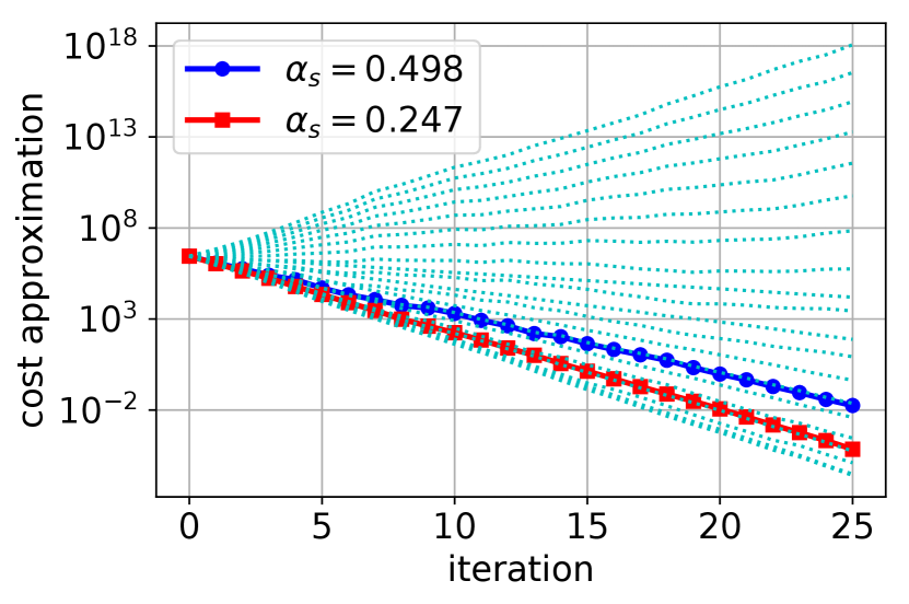
Figure 3 demonstrates that choosing when is calculated using the unbiased estimator formula leads to faster decrease of the objective value when the number of workers is high. If the number of workers is small, one should choose the step size that minimizes variance using instead. Furthermore, Figure 3(a) illustrates that the blue curve with square markers is in fact the best one could hope to achieve as it is very close to the best cyan dotted line.
V-B Distributed Newton Sketch for Regularized Problems
We now consider problems with squared -norm regularization. In particular, we study problems with Hessian matrices of the form . Sketching can be applied to obtain approximate Hessian matrices as . Note that the case corresponds to the setting in the GIANT algorithm described in [22].
Theorem V.2 establishes that should be chosen according to the formula (44) under the assumption that the singular values of are identical. We later verify empirically that when the singular values are not identical, plugging the mean of the singular values into the formula still leads to improvements over the case of .
Theorem V.2
Given the thin SVD decomposition and where is assumed to have full rank and satisfy , the bias of the single sketch Newton step estimator is equal to zero as goes to infinity when is chosen as
| (44) |
where and , and is the Gaussian sketch.
Remark V.3
The proof of Theorem V.2 builds on the proof of Theorem II.20 (see Appendix). The main difference between these results is that the setting in Theorem V.2 is such that we assume access to the full gradient, i.e. only the Hessian matrix is sketched. In contrast, the setting in Theorem II.20 does not use the exact gradient.
VI Applications of Distributed Sketching
This section describes some example problems where our methodology can be applied. In particular, the problems in this section are convex problems that are efficiently addressed by our methods in distributed systems. We present numerical results on these problems in Section VII.
VI-A Logistic Regression
We begin by considering the well-known logistic regression model with squared -norm penalty. The optimization problem for this model can be formulated as where
| (45) |
and is defined such that . denotes the ’th row of the data matrix . The output vector is denoted by .
We can use the distributed Newton sketch algorithm to solve this optimization problem. The gradient and Hessian for are as follows
is a diagonal matrix with the elements of the vector as its diagonal entries. The sketched Hessian matrix in this case can be formed as where can be calculated using (44), and we can set to the mean of the singular values of . Since the entries of the matrix are a function of the variable , the matrix gets updated every iteration. It might be computationally expensive to re-compute the mean of the singular values of in every iteration. However, we have found through experiments that it is not required to compute the exact value of the mean of the singular values for bias reduction. For instance, setting to the mean of the diagonals of the matrix as a heuristic works sufficiently well.
VI-B Inequality Constrained Optimization
The second application that we consider is the inequality constrained optimization problem of the form
| subject to | (46) |
where , and are the problem data, and is a positive scalar. Note that this problem is the dual of the Lasso problem given by .
The above problem can be tackled by the standard log-barrier method [33], by solving sequences of unconstrained barrier penalized problems as follows
| (47) |
where represents the ’th row of . The distributed Newton sketch algorithm could be used to solve this problem. The gradient and Hessian of the objective are given by
Here and is a diagonal matrix with the element-wise inverse of the vector as its diagonal entries. is the length- vector of all ’s. The sketched Hessian can be written in the form of .
Remark VI.1
Since the contribution of the regularization term in the Hessian matrix is , we need to plug instead of in the formula for computing .
VI-C Fine Tuning of Pre-Trained Neural Networks
The third application is neural network fine tuning. Let represent the output of the ’st layer of a pre-trained network which consists of layers. We are interested in re-using a pre-trained neural network for, say, a task on a different dataset by learning a different final layer. More precisely, assuming squared loss, one way that we can formulate this problem is as follows
| (48) |
where is the weight matrix of the final layer. The vectors denote the rows of the data matrix and is the output matrix. In a classification problem, would correspond to the number of classes.
For large scale datasets, it is important to develop efficient methods for solving the problem in (48). Distributed randomized ridge regression algorithm (listed in Algorithm 3) could be applied to this problem where the sketched sub-problems are of the form
| (49) |
and the averaged solution can be computed at the master node as . This leads to an efficient non-iterative asynchronous method for fine-tuning of a neural network.
VII Numerical Results
We have implemented the distributed sketching methods for AWS Lambda in Python using the Pywren package [34]. The setting for the experiments is a centralized computing model where a single master node collects and averages the outputs of the worker nodes. The majority of the figures in this section plots the approximation error which we define as .
VII-A Hybrid Sketch
In a distributed computing setting, the amount of data that can be fit into the memory of nodes and the size of the largest problem that can be solved by the nodes often do not match. The hybrid sketch idea is motivated by this mismatch and it is basically a sequentially concatenated sketching scheme where we first perform uniform sampling with dimension and then sketch the sampled data using another sketching method, preferably with better convergence properties (say, Gaussian) with dimension . Worker nodes load rows of the data matrix into their memory and then perform sketching, reducing the number of rows from to . In addition, we note that if , hybrid sketch reduces to sampling and if , then it reduces to Gaussian sketch. The hybrid sketching scheme does not take privacy into account as worker nodes are assumed to have access to the data matrix.
For the experiments involving very large scale datasets, we have used Sparse Johnson-Lindenstrauss Transform (SJLT) [24] as the second sketching method in the hybrid sketch due to its low computational complexity.
VII-B Airline Dataset
We have conducted experiments with the publicly available Airline dataset [35]. This dataset contains information on domestic USA flights between the years 1987-2008. We are interested in predicting whether there is going to be a departure delay or not, based on information about the flights. More precisely, we are interested in predicting whether DepDelay minutes using the attributes Month, DayofMonth, DayofWeek, CRSDepTime, CRSElapsedTime, Dest, Origin, and Distance. Most of these attributes are categorical and we have used dummy coding to convert these categorical attributes into binary representations. The size of the input matrix , after converting categorical features into binary representations, becomes .
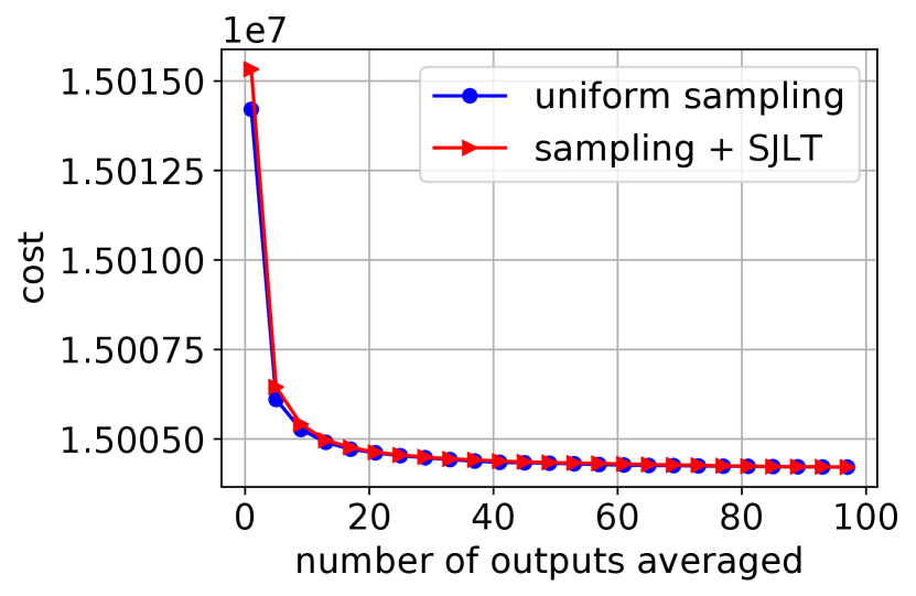
We have solved the linear least squares problem on the entire airline dataset: using workers on AWS Lambda. The output for the plots a and b in Figure 4 is a vector of binary variables indicating delay. The output for the plots c and d in Figure 4 is artificially generated via where is the underlying solution and is random Gaussian noise distributed as . Figure 4 shows that sampling followed by SJLT leads to a lower error.
We note that it increases the convergence rate to choose and as large as the available resources allow. Based on the run times given in the caption of Figure 4, we see that the run times are slightly worse if SJLT is involved. Decreasing will help reduce this processing time at the expense of error performance.

a)
b)

c)

d)
VII-C Image Dataset: Extended MNIST
The experiments of this subsection are performed on the image dataset EMNIST (extended MNIST) [36]. We have used the ”bymerge” split of EMNIST, which has 700K training and 115K test images. The dimensions of the images are and there are 47 classes in total (letters and digits). Some capital letter classes have been merged with small letter classes (like C and c), and thus there are 47 classes and not 62.

a) Approximation error

b) Test accuracy
Figure 5 shows the approximation error and test accuracy plots when we fit a least squares model on the EMNIST-bymerge dataset using the distributed randomized regression algorithm. Because this is a multi-class classification problem, we have one-hot encoded the labels. Figure 5 demonstrates that SJLT is able to drive the cost down more and leads to a better classification accuracy than uniform sampling.
VII-D Performance on Large Scale Synthetic Datasets
We now present the results of the experiments carried out on randomly generated large scale data to illustrate scalability of the methods. Plots in Figure 6 show the approximation error as a function of time, where the problem dimensions are as follows: for plot a and for plot b. These data matrices take up GB and GB, respectively. The data used in these experiments were randomly generated from the student’s t-distribution with degrees of freedom of for plot a and for plot b. The output vector was computed according to where is i.i.d. noise distributed as . Other parameters used in the experiments are for plot a, and for plot b. We observe that both plots in Figure 6 reveal similar trends where the hybrid approach leads to a lower approximation error but takes longer due to the additional processing required for SJLT.

a)

b)
VII-E Numerical Results for the Right Sketch Method
Figure 7 shows the approximation error as a function of the number of averaged outputs in solving the least norm problem for two different datasets. The dataset for Figure 7(a) is randomly generated with dimensions . We observe that Gaussian sketch outperforms uniform sampling in terms of the approximation error. Furthermore, Figure 7(a) verifies that if we apply the hybrid approach of sampling first and then applying Gaussian sketch, then its performance falls between the extreme ends of only sampling and only using Gaussian sketch. Moreover, Figure 7(b) shows the results for the same experiment on a subset of the airline dataset where we have included the pairwise interactions as features which makes this an underdetermined linear system. Originally, we had features for this dataset and if we include all terms as features, we would have a total of features, most of which are zero for all samples. We have excluded the all-zero columns from this extended matrix to obtain the final dimensions .

a) Random data

b) Airline data
VII-F Distributed Iterative Hessian Sketch
We have evaluated the performance of the distributed IHS algorithm on AWS Lambda. In the implementation, each serverless function is responsible for solving one sketched problem per iteration. Worker nodes wait idly once they finish their computation for that iteration until the next iterate becomes available. The master node is implemented as another AWS Lambda function and is responsible for collecting and averaging the worker outputs and broadcasting the next iterate .
Figure 8 shows the scaled difference between the cost for the ’th iterate and the optimal cost (i.e. ) against wall-clock time for the distributed IHS algorithm given in Algorithm 2. Due to the relatively small size of the problem, we have each worker compute the exact gradient without requiring an additional communication round per iteration to form the full gradient. We note that, for problems where it is not feasible for workers to form the full gradient due to limited memory, one can include an additional communication round where each worker sends their local gradient to the master node, and the master node forms the full gradient and distributes it to the worker nodes.

VII-G Inequality Constrained Optimization
Figure 9 compares the error performance of sketches with and without bias correction for the distributed Newton sketch algorithm when it is used to solve the log-barrier penalized problem given in (47). For each sketch, we have plotted the performance for and the bias corrected version (see Theorem V.2). The bias corrected versions are shown as the dotted lines. In these experiments, we have set to the minimum of the singular values of as we have observed that setting to the minimum of the singular values of performed better than setting it to their mean.
Even though the bias correction formula is derived for Gaussian sketch, we observe that it improves the performance of SJLT as well. We see that Gaussian sketch and SJLT perform the best out of the 4 sketches we have experimented with. We note that computational complexity of sketching for SJLT is lower than it is for Gaussian sketch, and hence the natural choice would be to use SJLT in this case.

VIII Discussion
In this work, we study averaging sketched solutions for linear least squares problems and averaging for randomized second order optimization algorithms. We discuss distributed sketching methods from the perspectives of convergence, bias, privacy, and distributed computing. Our results and numerical experiments suggest that distributed sketching methods offer a competitive straggler-resilient solution for solving large scale problems.
We have shown that for problems involving regularization, averaging requires a more detailed analysis compared to problems without regularization. When the regularization term is not scaled properly, the resulting estimators are biased, and averaging a large number of independent sketched solutions does not converge to the true solution. We have provided closed-form formulas for scaling the regularization coefficient to obtain unbiased estimators that guarantee convergence to the optimum.
Appendix A Proofs
This section contains the proofs for the lemmas and theorems stated in the paper.
A-A Proofs of Theorems and Lemmas in Section II
Proof:
Since the Gaussian sketch estimator is unbiased (i.e., ), Lemma IV.1 reduces to By Lemma II.1, the error of the averaged solution conditioned on the events that , can exactly be written as
Using Markov’s inequality, it follows that
The LHS can be lower bounded as
| (50) | ||||
| (51) |
where we have used the identity in (50) and the independence of the events in (51). It follows
Setting and plugging in , which holds for , we obtain
∎
Lemma A.1
For the Gaussian sketching matrix and the matrix whose columns are orthonormal, the smallest singular value of the product is bounded as:
| (52) |
This result follows from the concentration of Lipshitz functions of Gaussian random variables.
Proof:
We start by invoking a result on the concentration of Stieltjes transforms, namely Lemma 6 of [37]. This implies that
| (53) |
where . The matrix can be written as a sum of rank-1 matrices as follows:
| (54) |
where is the ’th row of . The vectors are independent as required by Lemma 6 of [37]. Next, we will bound the difference between the trace terms and . First, we let the SVD decomposition of be . Then, we have the following relations:
| (55) |
where the notation refers to a diagonal matrix with diagonal entries equal to . The difference between the trace terms can be bounded as follows:
| (56) |
Equivalently, we have
| (57) |
We know that . Using the upper bound yields
| (59) |
The concentration inequality in (A-A) and the concentration of the minimum singular value from Lemma A.1 together imply that
| (60) |
We now simplify this bound by observing that
| (61) |
where we used in the third line. We have also used the following simple inequality
| (62) |
For the fourth line to be true, we need . This is satisfied if or . We note that this is already implied by our assumption that . Using the above observation, we simplify the bound as follows:
| (63) |
Scaling gives
| (64) |
Setting and then give us the final result:
| (65) |
∎
Proof:
Let us consider the single sketch estimator . The relative error of can be expressed as
| (66) |
where the superscript indicates the pseudo-inverse. We will rewrite the error expression as:
| (67) |
and define and . This simplifies the previous expression
| (68) |
Lemma II.5 implies
| (69) |
The terms and reduce to the following expressions:
| (70) | ||||
| (71) |
Plugging these in (69) and taking the expectation of both sides with respect to give us
| (72) |
Next, we combine (72) with Lemma II.7 and the concentration of the minimum singular value from Lemma A.1 to obtain
| (73) |
Assuming that , we can write:
| (74) |
Making the change of variable yields:
| (75) |
Scaling yields:
| (76) |
Letting and , and then scaling lead to
| (77) |
Let us also set :
| (78) |
Under our assumption that , the above probability is bounded by
| (79) |
We now move on to find a lower bound. We note that Lemma II.5 can be used as follows to find a lower bound
| (80) |
Therefore, we have the following lower bound for the error:
| (81) |
Using the upper bound for and the exact expression for , and taking the expectation with respect to , we obtain the following
| (82) |
Applying the same steps as before, we arrive at the following bound:
| (83) |
∎
Proof:
Consider the averaged estimator :
| (84) |
where we defined
| (85) |
We note that the entries of the vector are distributed as i.i.d. standard normal. We can manipulate the error expression as follows
| (86) |
and then
| (87) |
We will now find an equivalent expression for :
| (88) |
where we have used the Cauchy-Schwarz inequality to bound the trace of the matrix product.
Next, we look at :
| (89) |
By Lemma II.5, we have
| (90) |
We can take expectation of both sides with respect to , to remove the conditioning. The expectation term inside the probability is equal to
| (91) |
Hence, we have
| (92) |
We now use the concentration bound of the trace term in Lemma II.7 to obtain
| (93) |
where we have used the independence of ’s. Using the upper bounds for and , we make the following observation. If the minimum singular values of all of , satisfy , which occurs with probability at least from Lemma A.1, then the following holds
| (94) |
where we used and in the last two inequalities. Combining this observation with the probability bound, we arrive at
| (95) |
Simplifying the expressions and making the change lead to
| (96) |
Next, we let and obtain
| (97) |
We now set and scale :
| (98) |
Let us use the assumption to further simplify:
| (99) |
We can use Bernoulli’s inequality and arrive at:
| (100) |
where we also set . Picking yields:
| (101) |
Finally, we obtain the following simpler expression for the bound:
| (102) |
where we redefine the constants .
Lower bound can be obtained by applying the same steps:
| (103) |
∎
Proof:
i) For unbiased estimators: We begin by invoking Lemma IV.1 which gives us
| (104) |
since we assume that ’s are unbiased, i.e., for .
This shows that the error of the averaged estimator is equal to the error of the single sketch estimator scaled by . Hence, we can leverage the lower bound result for the single sketch estimator. We now give the details of how to find the lower bound for the single sketch estimator which was first shown in [28].
The Fisher information matrix for estimating from can be constructed as follows:
| (105) |
where is the probability density function of conditioned on , i.e., is the multivariate Gaussian distribution with . We recall the definition that .
The gradient of the logarithm of the probability density function with respect to is
| (106) |
Plugging this in (105) yields
| (107) |
We note that the expectation of the error conditioned on is equivalent to
| (108) |
where the last line follows from the Cramér lower bound [38] given by
| (109) |
Taking the expectation of both sides with respect to yields
| (110) |
Hence, we arrive at
| (111) |
Proof:
The update rule for distributed IHS is given as
| (113) |
Let us decompose as and note that which gives us:
| (114) |
Subtracting from both sides, we obtain an equation in terms of the error vector only:
Let us multiply both sides by from the left and define and we will have the following equation:
We now analyze the expectation of norm of :
| (115) |
The contribution for in the double summation of (A-A) is equal to zero because for , we have
The term in the last line above is zero for :
where we used . For the rest of the proof, we assume that we set . Now that we know the contribution from terms with is zero, the expansion in (A-A) can be rewritten as
The term can be simplified using SVD decomposition . This gives us and furthermore we have:
Plugging this in, we obtain:
∎
Proof:
Taking the expectation with respect to the sketching matrices , of both sides of the equation given in Theorem II.13, we obtain
This gives us the relationship between the initial error (when we initialize to be the zero vector) and the expected error in iteration :
It follows that the expected error reaches -accuracy with respect to the initial error at iteration where:
Each iteration requires communicating a -dimensional vector for every worker, and we have workers and the algorithm runs for iterations, hence the communication load is .
The computational load per worker at each iteration involves the following numbers of operations:
-
•
Sketching : multiplications
-
•
Computing : multiplications
-
•
Computing : operations
-
•
Solving : operations.
∎
Proof:
In the following, we assume that we are in the regime where approaches infinity.
The expectation term is equal to the identity matrix times a scalar (i.e. ) because it is signed permutation invariant, which we show as follows. Let be a permutation matrix and be an invertible diagonal sign matrix ( and ’s on the diagonals). A matrix is signed permutation invariant if . We note that the signed permutation matrix is orthogonal: , which we later use in the sequel.
where we made the variable change and note that has orthonormal columns because is an orthogonal transformation. and have the same distribution because is an orthogonal transformation and is a Gaussian matrix. This shows that is signed permutation invariant.
Now that we established that is equal to the identity matrix times a scalar, we move on to find the value of the scalar. We use the identity for where the diagonal entries of are sampled from the Rademacher distribution and is sampled uniformly from the set of all possible permutation matrices. We already established that is equal to for any signed permutation matrix of the form . It follows that
where we define to be the set of all possible signed permutation matrices in going from line 1 to line 2.
By Lemma II.18, the trace term is equal to , which concludes the proof. ∎
Proof:
Closed form expressions for the optimal solution and the output of the ’th worker are as follows:
Equivalently, can be written as:
This allows us to decompose as
where with and . From the above equation we obtain and .
The bias of is given by (omitting the subscript in for simplicity)
By the assumption , the bias becomes
| (116) |
The first expectation term of (116) can be evaluated using Lemma II.19 (as goes to infinity):
| (117) |
To find the second expectation term in (116), let us first consider the full SVD of given by where and . The matrix is an orthogonal matrix, which implies . If we insert between and , the second term of (116) becomes
In these derivations, we used . This follows from as and are orthogonal. The last line follows from Lemma II.19, as goes to infinity.
We note that and for , this becomes . Bringing the pieces together, we have the bias equal to (as goes to infinity):
If there is a value of that satisfies , then that value of makes an unbiased estimator. Equivalently,
| (118) |
where we note that the LHS is a monotonically increasing function of in the regime and it attains its minimum in this regime at . Analyzing this equation using these observations, for the cases of and separately, we find that for the case of , we need the following to be satisfied for zero bias:
whereas there is no additional condition on for the case of .
The value of that will lead to zero bias can be computed by solving the equation (118) where the expression for the inverse of the left-hand side is given by . We evaluate the inverse at and obtain the following expression for :
∎
A-B Proofs of Theorems and Lemmas in Section III
The proof of the privacy result mainly follows due to Theorem A.2 (stated below for completeness) which is a result from [39].
Proof:
For some , and matrix , if there exist values for such that the smallest singular value of satisfies , then using Theorem A.2, we find that the sketch size has to satisfy the following for -differential privacy:
| (119) |
where we have set in the second line. For the first line to follow from Theorem A.2, we also need the condition to be satisfied. Note that the rows of have bounded -norm of . We now substitute and to obtain the simplified condition
where and are constants. Assuming this condition is satisfied, then we pick the sketch size as (A-B) which can also be simplified:
Note that the above arguments are for the privacy of a single sketch (i.e., ). In the distributed setting where the adversary can attack all of the sketched data , we can consider all of the sketched data to be a single sketch with size . Based on this argument, we can pick the sketch size as
∎
Theorem A.2 (Differential privacy for random projections [39])
Fix and . Fix . Fix a positive integer and let be such that
| (120) |
Let be an -matrix with and where each row of has bounded -norm of . Given that , the algorithm that picks an -matrix whose entries are iid samples from the normal distribution and publishes the projection is -differentially private.
A-C Proofs of Theorems and Lemmas in Section IV
Proof:
The expectation of the difference between the costs and is given by
| (121) |
where we have used the orthogonality property of the optimal least squares solution given by the normal equations . Next, we have
∎
Proof:
The bias of the single sketch estimator can be expanded as follows:
where we define and . The term can be upper bounded as follows when conditioned on the event :
where the inequality follows from the inequality and some simple bounds for the minimum and maximum eigenvalues of the product of two positive definite matrices. Furthermore, the expectation of is equal to zero because . Hence we obtain the claimed bound ∎
Proof:
For the randomized Hadamard sketch (ROS), the term can be expanded as follows. We will assume that all the expectations are conditioned on the event , which we defined earlier as .
where we have used the independence of and , . This is true because of the assumption that the matrix corresponds to sampling with replacement.
where the row vector corresponds to the ’th row of the Hadamard matrix . We also note that the expectation in the last line is with respect to the randomness of .
Let us define to be the column vector containing the diagonal entries of the diagonal matrix , that is, . Then, the vector is equivalent to where is the diagonal matrix with the entries of on its diagonal.
where we have defined . It follows that . Here, is used to refer to the diagonal matrix with the diagonal entries of as its diagonal. The trace of can be easily computed using the cyclic property of matrix trace as . Next, we note that the term can be simplified as where is the ’th row of . This leads to
Going back to , we have
∎
Proof:
We will assume that all the expectations are conditioned on the event , which we defined earlier as . For uniform sampling with replacement, we have
Next, for uniform sampling without replacement, the rows and are not independent which can be seen by noting that given , we know that will have its nonzero entry at a different place than . Hence, differently from uniform sampling with replacement, the following term will not be zero:
It follows that for uniform sampling without replacement, we obtain
∎
Proof:
We consider leverage score sampling with replacement. The rows , are independent because sampling is with replacement. We will assume that all the expectations are conditioned on the event , which we defined earlier as . For leverage score sampling, the term is upper bounded as follows:
∎
Proof:
We will begin by using the results from Table 5 of [3] for selecting the sketch size:
| (122) |
where is the row coherence of as defined before. When the sketch sizes are selected according to the formulas above, the subspace embedding property given by
| (123) |
is satisfied with probability at least . Note that the subspace embedding property can be rewritten as
| (124) |
This implies the following relation for the inverse matrix :
| (125) |
Observe that for any and that for . Assuming that , we have
| (126) |
We can rescale so that
| (127) |
and the effect of this rescaling will be hidden in the notation for the sketch size formulas.
We will define the events , as and it follows that when the sketch sizes are selected according to (A-C), we will have
| (128) |
Now, we find a simpler expression for the error of the single-sketch estimator:
| (129) |
where we defined , and . The variance term is equal to
| (130) |
Conditioned on the event , we can bound the expectation as follows:
| (131) |
where we have used , which follows from all eigenvalues of being less than when conditioned on the event . Next, from Lemma IV.1, we obtain the following bound for the expected error
| (132) |
Using Markov’s inequality gives us the following probability bound:
| (133) |
The unconditioned probability can be computed as
| (134) |
where we have used and . We can obtain a bound for the relative error as follows:
| (135) |
Scaling leads to
| (136) |
A-D Proofs of Theorems and Lemmas in Section V
Proof:
The optimal update direction is given by
and the estimate update direction due to a single sketch is given by
where is the step size scaling factor to be determined. Letting be a Gaussian sketch, the bias can be written as
In the third line, we plug in the mean of which is distributed as inverse Wishart distribution (see Lemma A.3). This calculation shows that the single sketch estimator gives an unbiased update direction for .
The variance analysis is as follows:
Plugging into the first term and assuming has full column rank, the expectation term becomes
where the third line follows due to Lemma A.3. Because , the variance becomes:
It follows that the variance is minimized when is chosen as . ∎
Lemma A.3 ([40])
For the Gaussian sketch matrix with i.i.d. entries distributed as where , and for with , the following are true:
| (141) |
where and are defined as
| (142) |
Proof:
In the following, we omit the subscripts in for simplicity. Using the SVD decomposition of , the bias can be written as
By the assumption that , the bias term can be simplified as
By Lemma II.19, as goes to infinity, we have
The bias becomes zero for the value of that satisfies the following equation:
| (143) |
In the regime where , the LHS of (143) is always non-negative and is monotonically decreasing in .The LHS approaches zero as . We now consider the following cases:
-
•
Case 1: . Because , as , the LHS goes to infinity. Since the LHS can take any values between and , there is an appropriate value that makes the bias zero for any .
-
•
Case 2: . In this case, . The maximum of LHS in this case is reached as and it is equal to . As long as is true, then we can drive the bias down to zero. More simply, this corresponds to , which is always true. Therefore in the case of as well, there is a value for any value of that will drive the bias down to zero.
To sum up, for any given value for the regularization parameter , it is possible to find a value to make the sketched update direction unbiased. The optimal value for is given by where , which simplifies to the following expression:
∎
Appendix B Additional Numerical Results
In this section, we present additional experimental results.
B-A Scalability of the Serverless Implementation
Figure 10 shows the cost against time when we solve the problem given in (47) for large scale data on AWS Lambda using the distributed Newton sketch algorithm. The setting in this experiment is such that each worker node has access to a different subset of data, and there is no additional sketching applied. The dataset used is randomly generated and the goal here is to demonstrate the scalability of the algorithm and the serverless implementation. The size of the data matrix is GB.

In the serverless computing implementation, we reuse the serverless functions during the course of the algorithm, meaning that the same functions are used for every iteration. We note that every iteration requires two rounds of communication with the master node. The first round is for the communication of the local gradients, and the second round is for the approximate update directions. The master node, also a serverless function, is also reused across iterations. Figure 10 illustrates that each iteration takes a different amount of time and iteration times can be as short as seconds. The reason for some iterations taking longer times is what is referred to as the straggler problem, which is a phenomenon commonly encountered in distributed computing. More precisely, the iteration time is determined by the slowest of the nodes and nodes often slow down for a variety of reasons causing stragglers. A possible solution to the issue of straggling nodes is to use error correcting codes to insert redundancy to computation and hence to avoid waiting for the outputs of all of the worker nodes [41, 42]. We identify that implementing straggler mitigation for solving large scale problems via approximate second order optimization methods such as distributed Newton sketch is a promising direction.
B-B Experiments on UCI Datasets
In the case of large datasets and limited computing resources of worker nodes such as memory and lifetime, most of the standard sketches are computationally too expensive as discussed in the main body of the paper. This is the reason why we limited the scope of the large scale experiments to uniform sampling, SJLT, and hybrid sketch. In this section we present some additional experimental results on smaller datasets to empirically verify the theoretical results of the paper.
We present results on two UCI datasets in Figure 11 comparing the performances of the sketches we discussed in the paper.

a) echocardiogram

b) oocytes merluccius nucleus
Figure 11 shows that Gaussian and ROS sketches lead to unbiased estimators in the experiments because the corresponding curves appear linear in the log-log scale plots. These experiment results suggest that the upper bound that we have found for the bias of the ROS sketch may not be tight. We see that the estimates for uniform sampling and leverage score sampling are biased. The observation that the Gaussian sketch estimator is unbiased in the experiments is perfectly consistent with our theoretical findings. Furthermore, we observe that the approximation error is the highest in uniform sampling, which is also in agreement with the theoretical upper bounds that we have presented.
References
- [1] C.-C. Wang, K. L. Tan, C.-T. Chen, Y.-H. Lin, S. S. Keerthi, D. Mahajan, S. Sundararajan, and C.-J. Lin, “Distributed newton methods for deep neural networks,” Neural Comput., vol. 30, no. 6, p. 1673–1724, Jun. 2018. [Online]. Available: https://doi.org/10.1162/neco_a_01088
- [2] P. Drineas, M. W. Mahoney, S. Muthukrishnan, and T. Sarlós, “Faster least squares approximation,” Numerische mathematik, vol. 117, no. 2, pp. 219–249, 2011.
- [3] S. Wang, A. Gittens, and M. W. Mahoney, “Sketched ridge regression: Optimization perspective, statistical perspective, and model averaging,” J. Mach. Learn. Res., vol. 18, no. 1, pp. 8039–8088, Jan. 2017.
- [4] M. Pilanci and M. J. Wainwright, “Iterative hessian sketch: Fast and accurate solution approximation for constrained least-squares,” The Journal of Machine Learning Research, vol. 17, no. 1, pp. 1842–1879, 2016.
- [5] J. Lacotte and M. Pilanci, “Faster least squares optimization,” arXiv preprint, arXiv:1911.02675, 2019.
- [6] M. W. Mahoney, “Randomized algorithms for matrices and data,” Foundations and Trends in Machine Learning in Machine Learning, vol. 3, no. 2, 2011.
- [7] M. Pilanci and M. J. Wainwright, “Randomized sketches of convex programs with sharp guarantees,” IEEE Trans. Info. Theory, vol. 9, no. 61, pp. 5096–5115, September 2015.
- [8] D. Bertsekas and J. Tsitsiklis, Parallel and Distributed Computation: Numerical Methods. Prentice-Hall, 1989.
- [9] F. Niu, B. Recht, C. Re, and S. J. Wright, “Hogwild! a lock-free approach to parallelizing stochastic gradient descent,” in Proceedings of the 24th International Conference on Neural Information Processing Systems, ser. NIPS’11. Red Hook, NY, USA: Curran Associates Inc., 2011, p. 693–701.
- [10] S. Zhou, J. Lafferty, and L. Wasserman, “Compressed and privacy-sensitive sparse regression,” IEEE Transactions on Information Theory, vol. 55, no. 2, pp. 846–866, Feb 2009.
- [11] M. Showkatbakhsh, C. Karakus, and S. Diggavi, “Privacy-utility trade-off of linear regression under random projections and additive noise,” in 2018 IEEE International Symposium on Information Theory (ISIT), June 2018, pp. 186–190.
- [12] S. Zhou, J. Lafferty, and L. Wasserman, “Compressed regression,” in Neural Information Processing Systems, December 2007.
- [13] J. Blocki, A. Blum, A. Datta, and O. Sheffet, “The johnson-lindenstrauss transform itself preserves differential privacy,” in 2012 IEEE 53rd Annual Symposium on Foundations of Computer Science, 2012, pp. 410–419.
- [14] S. S. Vempala, The random projection method. American Mathematical Soc., 2005, vol. 65.
- [15] M. W. Mahoney, “Randomized algorithms for matrices and data,” Foundations and Trends® in Machine Learning, vol. 3, no. 2, pp. 123–224, 2011.
- [16] D. P. Woodruff et al., “Sketching as a tool for numerical linear algebra,” Foundations and Trends® in Theoretical Computer Science, vol. 10, no. 1–2, pp. 1–157, 2014.
- [17] P. Drineas and M. W. Mahoney, “RandNLA: randomized numerical linear algebra,” Communications of the ACM, vol. 59, no. 6, pp. 80–90, 2016.
- [18] H. Avron, P. Maymounkov, and S. Toledo, “Blendenpik: Supercharging lapack’s least-squares solver,” SIAM Journal on Scientific Computing, vol. 32, no. 3, pp. 1217–1236, 2010.
- [19] V. Rokhlin, A. Szlam, and M. Tygert, “A randomized algorithm for principal component analysis,” SIAM Journal on Matrix Analysis and Applications, vol. 31, no. 3, pp. 1100–1124, 2009.
- [20] M. Pilanci and M. J. Wainwright, “Randomized sketches of convex programs with sharp guarantees,” IEEE Transactions on Information Theory, vol. 61, no. 9, pp. 5096–5115, 2015.
- [21] ——, “Newton sketch: A near linear-time optimization algorithm with linear-quadratic convergence,” SIAM Journal on Optimization, vol. 27, no. 1, pp. 205–245, 2017.
- [22] S. Wang, F. Roosta, P. Xu, and M. W. Mahoney, “Giant: Globally improved approximate newton method for distributed optimization,” in Advances in Neural Information Processing Systems 31. Curran Associates, Inc., 2018, pp. 2332–2342.
- [23] T. Sarlos, “Improved approximation algorithms for large matrices via random projections,” in Foundations of Computer Science, 2006. FOCS’06. 47th Annual IEEE Symposium on. IEEE, 2006, pp. 143–152.
- [24] J. Nelson and H. L. Nguyên, “Osnap: Faster numerical linear algebra algorithms via sparser subspace embeddings,” in Foundations of Computer Science (FOCS), 2013 IEEE 54th Annual Symposium on. IEEE, 2013, pp. 117–126.
- [25] G. Letac and H. Massam, “All invariant moments of the wishart distribution,” Scandinavian Journal of Statistics, vol. 31, no. 2, pp. 295–318, 2004.
- [26] D. C. Ahfock, W. J. Astle, and S. Richardson, “Statistical properties of sketching algorithms,” Biometrika, vol. 108, no. 2, pp. 283–297, 07 2020. [Online]. Available: https://doi.org/10.1093/biomet/asaa062
- [27] S. Boucheron, G. Lugosi, and P. Massart, Concentration Inequalities - A Nonasymptotic Theory of Independence. Oxford University Press, 2013.
- [28] S. Sridhar, M. Pilanci, and A. Özgür, “Lower bounds and a near-optimal shrinkage estimator for least squares using random projections,” IEEE Journal on Selected Areas in Information Theory, vol. 1, no. 3, pp. 660–668, 2020.
- [29] S. Liu and E. Dobriban, “Ridge regression: Structure, cross-validation, and sketching,” 2019.
- [30] C. Dwork, K. Kenthapadi, F. McSherry, I. Mironov, and M. Naor, “Our data, ourselves: Privacy via distributed noise generation,” in Proceedings of the 24th Annual International Conference on The Theory and Applications of Cryptographic Techniques, ser. EUROCRYPT’06. Berlin, Heidelberg: Springer-Verlag, 2006, p. 486–503. [Online]. Available: https://doi.org/10.1007/11761679_29
- [31] O. Sheffet, “Private approximations of the 2nd-moment matrix using existing techniques in linear regression,” CoRR, vol. abs/1507.00056, 2015. [Online]. Available: http://arxiv.org/abs/1507.00056
- [32] Z. Huang, S. Mitra, and N. Vaidya, “Differentially private distributed optimization,” in Proceedings of the 2015 International Conference on Distributed Computing and Networking, ser. ICDCN ’15. New York, NY, USA: Association for Computing Machinery, 2015. [Online]. Available: https://doi.org/10.1145/2684464.2684480
- [33] S. Boyd and L. Vandenberghe, Convex optimization. Cambridge university press, 2004.
- [34] E. Jonas, S. Venkataraman, I. Stoica, and B. Recht, “Occupy the cloud: Distributed computing for the 99%,” CoRR, vol. abs/1702.04024, 2017. [Online]. Available: http://arxiv.org/abs/1702.04024
- [35] B. of Transportation Statistics, “Airline on-time statistics and delay causes, http://stat-computing.org/dataexpo/2009/,” 2018.
- [36] G. Cohen, S. Afshar, J. Tapson, and A. van Schaik, “EMNIST: an extension of MNIST to handwritten letters,” CoRR, vol. abs/1702.05373, 2017. [Online]. Available: http://arxiv.org/abs/1702.05373
- [37] N. E. Karoui, “Concentration of measure and spectra of random matrices: Applications to correlation matrices, elliptical distributions and beyond,” The Annals of Applied Probability, vol. 19, no. 6, pp. 2362–2405, 2009.
- [38] A. A. Borovkov, Mathematical statistics. Australia: Gordon and Breach Science Publishers, 1998.
- [39] O. Sheffet, “Private approximations of the 2nd-moment matrix using existing techniques in linear regression,” CoRR, vol. abs/1507.00056, 2015. [Online]. Available: http://arxiv.org/abs/1507.00056
- [40] J. Lacotte and M. Pilanci, “Faster least squares optimization,” arXiv preprint, arXiv:1911.02675, 2019.
- [41] K. Lee, M. Lam, R. Pedarsani, D. Papailiopoulos, and K. Ramchandran, “Speeding up distributed machine learning using codes,” IEEE Transactions on Information Theory, vol. 64, no. 3, pp. 1514–1529, March 2018.
- [42] B. Bartan and M. Pilanci, “Straggler resilient serverless computing based on polar codes,” in 2019 57th Annual Allerton Conference on Communication, Control, and Computing (Allerton), 2019, pp. 276–283.