Distributed Networked Real-time Learning
Abstract
Many machine learning algorithms have been developed under the assumption that data sets are already available in batch form. Yet in many application domains data is only available sequentially overtime via compute nodes in different geographic locations. In this paper, we consider the problem of learning a model when streaming data cannot be transferred to a single location in a timely fashion. In such cases, a distributed architecture for learning relying on a network of interconnected “local” nodes is required. We propose a distributed scheme in which every local node implements stochastic gradient updates based upon a local data stream. To ensure robust estimation, a network regularization penalty is used to maintain a measure of cohesion in the ensemble of models. We show the ensemble average approximates a stationary point and characterize the degree to which individual models differ from the ensemble average. We compare the results with federated learning to conclude the proposed approach is more robust to heterogeneity in data streams (data rates and estimation quality). We illustrate the results with an application to image classification with a deep learning model based upon convolutional neural networks.
keywords: asynchronous computing, distributed computing, networks, non-convex optimization, real-time machine learning.
1 Introduction
Streaming data sets are pervasive in certain application domains often involving a network of compute nodes located in different geographic locations. However, most machine learning algorithms have been developed under the assumption that data sets are already available in batch form. When the data is obtained through a network of heterogeneous compute nodes, assembling a diverse batch of data points in a central processing location to update a model may imply significant latency. Recently, an architecture referred to as federated learning (FL, see e.g. [1, 2]) with a central server in proximity to local nodes has been proposed. In FL, each node implements updates to a machine learning model that is kept in the central server. This allows collaborative learning while keeping all the training data on nodes rather than in the cloud. In general, schemes that avoid the need to rely on the cloud for data storage and/or computation are referred to as “edge computing”.
With high data payloads, such architecture for real-time learning is subject to an accuracy vs speed trade-off due to asymmetries in data quality vs. data rates as we explain in what follows.
Consider nodes generating data points at different rates which are used for the instantaneous computation of model updates (striving to minimize loss ). This setting could correspond for example with supervised deep learning in real-time wherein gradient estimates (with noise variance ) are computed via back-propagation in a relatively fast fashion. Without complete information on , updating the model parameters based upon every incoming data point yields high speed but possibly at the expense of low accuracy. For example, if the nodes producing noisier estimates are also faster at producing data, it is highly unlikely that an accurate model will be identified at all.
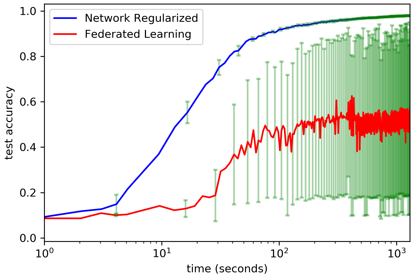
To illustrate this scenario, in Figure 1, we depict the performance of FL for deep convolutional neural networks with the MNIST dataset. In these simulations, each one of nodes sends data according to independent Poisson processes with and , . The fastest node computes gradient estimates based upon a single image whereas the slower nodes compute gradient estimates based upon a batch of images.
This trade-off between speed and precision is mitigated in a distributed approach to real-time learning subject to a network regularization penalty. In such an approach, each one of local nodes independently produce parameter updates based upon a single (locally obtained) data point which speeds up computation. Evidently, with increased noise, such a scheme may fail to enable the identification of a reasonably accurate model. However, by adding a network regularization penalty (which is computed locally) a form of coordination between multiple local nodes is induced so that the ensemble average solution is robust to noise.111Similar network regularization methods have been used in multi-task learning to account for inherent network structure in data sets (see e.g.[3, 4, 5, 6, 7, 8]). See section D. Specifically, we show that the ensemble average solution approximates a stationary point and that the approximation quality is , which compares quite favorably with FL, which is highly sensitive to fast and inaccurate data streams. We illustrate the results with an application to deep learning with convolutional neural networks.
The structure of the paper is as follows. In section 2 we introduce the distributed scheme that combines stochastic gradient descent with network regularization (NR). In section 3 we analyze the scheme and show that it converges (in a certain sense) to a stationary point, we also compare its performance with FL. Finally, in section 4 we report the results from a testbed on deep learning application to image processing, and in section 5 we offer conclusions.
2 A Network Regularized Approach to Real-time Learning
2.1 Setup
We consider a setting in which data is made available sequentially overtime via nodes in different geographic locations. We denote the -th stream by and assume these data points are independent samples from a joint distribution .
We also assume the data streams are independent but heterogeneous, i.e. . Each node strives to find a parameter specification that minimizes the performance criteria , where the loss function is continuously differentiable with respect to . Though data is distributed and heterogeneous, we consider a setting in which nodes agree on a common learning task. This is formalized in the first standing assumption. Let denote the gradient evaluated at , and assume is uniformly integrable.
Assumption 0: For all , and :
Let denote the (ensemble) average expected loss:
By uniform integrability, . Assumption 0 thus implies that for all and .
Let , then it holds that . We further assume:
Assumption 1: For all , the random variables are independent and
Define . By independence of data streams:
for all .
Streams generate data over time according to independent Poisson processes with rate and . We assume the time required to compute gradient estimates and/or exchange parameters locally among neighbors or with the central server are negligible compared to the time in between model updates. In what follows we make use of a virtual clock that produces ticks according to an aggregate counting process with rate . Let denote the index set of ticks associated with the aggregate process. Since we assume the parameter is updated once a data point arrives, the -th iteration is completed at the -th tick. Index denotes the -th step in the schemes described below.
2.2 Federated Real-time Learning
In FL, gradient estimates are communicated to a central server where a model is updated as follows:
| (1) |
where is the learning rate, is a indicator of whether node performs the an update: if the next gradient estimate comes from the -th stream and otherwise.
The algorithmic scheme described in (1) was first analyzed in [9] for data in batch form and has been used in the recent literature on asynchronous parallel optimization algorithms (see for example [10], [11] and [12]). As Figure 1 suggests, with heterogeneous data streams, the scheme in (1) trades off speed in producing parameter updates at the expense of heterogeneous noise in gradient estimates. In what follows we introduce a distributed approach that relies on a network regularization penalty to ensure the ensemble average approximates a stationary point (i.e. a choice of parameters with null gradient). We will show that in such a networked approach the trade-off between precision and speed is mitigated.
2.3 A Distributed Approach with Network Regularization
In the NR scheme, we consider a network of local compute nodes which we model as a graph , where stands for the set of nodes and is the set of links connecting nodes. Let be the adjacency matrix of , where indicates whether node communicates with node : if two nodes can exchange local information and otherwise.
In this scheme, each local node performs model updates according to a linear combination of local gradient estimate and the gradient of a consensus potential:
where . The consensus potential is a measure of similarity across local models.222This consensus potential has been used in the literature of opinion dynamics (see e.g. [13]). The update performed by node is of the form:
| (2) |
where is a regularization parameter, and
Note that the basic iterate (2) can be interpreted as a stochastic gradient approach to solve the local problem:
in which the objective function is a linear combination of loss and consensus potential.333This interpretation is not novel (see e.g. [14], [15] for its use in swarm (flocking) optimization and in multi-task learning [4, 5, 6, 7, 8]). When , each local node ignores the neighboring models. For large values of , the resulting dynamics reflect the countervailing effects of seeking to minimize consensus potential and improving model fit. With highly dissimilar initial models, each local node largely ignores its own data and opts for updates that lead to a model that is similar to the local average. Once approximate consensus is achieved, local gradient estimates begin to dictate the dynamics of model updates.
2.4 Literature Review
The scheme proposed in (2) has already been considered in the machine learning literature. In a series of papers (see [4, 5, 6, 7, 8])), the authors consider an approach to multi-task learning based upon a network regularization penalty as in (2). This paper focuses on distributed single-task learning. In contrast to the papers referred above, we consider a non-convex setting with heterogeneous nodes asynchronously updating their respective models at different rates over time.
The scheme proposed in (2) is also related to the literature on consensus optimization (see e.g. [17], [11], [18]). However, the proposed approach can not be interpreted as being based upon averaging over local models as in consensus-based optimization. In that literature, the basic iteration is of the form:
where is doubly stochastic and is a noisy gradient estimate. Indeed one can rewrite (2) as:
with and . However, the resulting matrix is not doubly stochastic in general since we only require . Thus, the approach to consensus in (2) can not be interpreted as being based upon averaging over local models as in consensus-optimization.
The algorithms proposed in [11] and [18] are designed for batch data while our approach deals with streaming data. For example, in [11], each node uses the same mini-batch size for estimating gradients while in our approach gradient estimation noise is heterogeneous. In addition, the algorithms proposed in [11] and [18], every node is equally likely to be selected at each iteration to update its local model. In contrast, in our approach data streams are heterogeneous so that certain nodes are more likely to update their models at any given time. Finally, in [11] the objective function (loss) is defined with respect to a distribution that is biased towards the nodes that update more often. This is in contrast to the objective function defined in this paper (i.e. ), where every node contributes to the global distribution with the same weight regardless of their updating frequency.
3 Analysis
In this section, we show the NR scheme converges (in a certain sense) to a stationary point. To that end we study stochastic processes associated with each one of the nodes in the network regularized approach. The proofs are given in the appendix. We make the following standing assumptions:
Assumption 2: The graph corresponding to the network of nodes is undirected () and connected, i.e., there is a path between every pair of vertices.
Assumption 3 (Lipschitz) for some and for all .
3.1 Preliminaries
The ensemble average plays an important role in characterizing the performance of the network regularized scheme. To this end, we analyze the process defined as
Let and , then . We now introduce some additional notations. Let denote the degree of vertex in graph and . Let denote the conditional expectation of given . We define and . We first prove two intermediate results.
Lemma 1 Suppose Assumptions 0, 1 and 2 hold. It holds that
where , and
Lemma 2 Suppose Assumptions 0, 1, 2 and 3 hold. Let , then:
where denotes the second-smallest of the Laplacian associated with graph and
3.2 Convergence
We are now ready to state and prove the main theorem.
As in [19], convergence is described in terms of the expected value of the average squared norm of the gradient in the first -updates. The ensuing corollary goes into further detail by describing the same result in terms of real-time elapsed and not just on a total number of iterations.
Theorem 1: Suppose Assumptions 0, 1, 2 and 3 hold. Choose , where
are positive by choosing . With scheme (2), it holds that
where .
The regularization penalty parameter must be high enough to ensure cohesion between local models. This condition is weaker with a higher degree of connectivity (i.e. higher values of ).
Note also that for fixed , when , then . So convergence, as characterized by Theorem 1, may be slower. This is not necessarily the case since the conditions in Theorem 1 identify a wide range of choices for and . For example, simulations indicate that for fixed higher values of may speed up convergence (see Figure 3 (c)).
3.3 Real-time Performance
The analysis in Theorem 1 takes place in the time scale indexed by and associated with the clicks associated with a Poisson process with rate . To embed the result in Theorem 1 in real-time, recall that is the counting process governing the aggregation of all data streams. Given our assumption on computation times being negligible, the total number of updates completed in is also . Let us define the conditional average squared gradient norm in the interval as follows:
| (4) |
Hence, the result in Theorem 1 can be reinterpreted by taking expectation of (4) over as:
According to Theorem 1, and using , the coupling of solutions via the network regularization penalty implies the ensemble average approximates a stationary point in the sense that:
The approximation quality is monotonically increasing in the number of nodes. The convergence properties outlined above are related to the ensemble average. It is, therefore, necessary to examine the degree to which individual models differ from the ensemble average. This is the gist of the next result.
Corollary 1: With the same assumptions and definitions in Theorem 1, it holds that
We embed the result in Corollary 1 in real-time. Define the conditional average of in the interval as
The random process tracks the average distance of individual models to the ensemble average. Similar to the discussion of Theorem 1, the real-time result of Corollary 1 is as follows:
This implies the asymptotic difference between individual models and the ensemble average satisfies:
The network regularization parameter plays an important role in controlling the upper bound of in Corollary 1. For fixed , when , then and , it follows that . Hence, the upper bound in Corollary 1 can be made arbitrarily small by choosing large enough .
3.4 Comparison to Federated Learning
We now present the counterpart convergence result regarding to FL.
Proposition 1: Suppose Assumptions 0, 1, 2 and 3 hold. For scheme 1, with a choice , it holds that:
with .
To embed the process in Proposition 1 in real-time, let us define the average squared gradient norm in the interval as follows:
| (5) |
Hence, the result in Proposition 1 can be reinterpreted by taking expectation of (5) over as:
To compare FL with NR, we also make . The asymptotic approximation quality is given by:
which suggests that the approximation quality is determined by the faster data streams. This leads to unsatisfactory performance whenever (i.e. faster data streams are also less accurate). Evidently, the opposite holds true when faster nodes are also more accurate, i.e. . However, in many real-time machine learning applications, this is not likely to be the case. Obtaining higher precision gradient estimates requires larger batches and/or increased computation. Thus nodes with higher precision are less likely to be the faster ones.
4 Testbed: Realtime Deep Learning
In this section, we report the results of NR (scheme (2)) to distributed real-time learning from three aspects: the comparison with FL (scheme (1)), the effects of the regularization parameter , and the effects of the network connectivity.
The specific learning task is to classify handwritten digits between and digits as given in the MNIST data set [20]. The dataset is composed of testing items and training items. Each item in the dataset is a black-and-white (single-channel) image of 28 28 pixels of a handwritten digit between and .
In the first two experiments, we implement schemes in a heterogeneous setting with nodes, and the third experiment with nodes in a homogeneous setting. In the test-bed MNIST streams according to independent Poisson processes. Gradient estimates are obtained with different mini-batch sizes. Evidently, a smaller mini-batch size implies noisier gradient estimates. The detailed experimental settings are summarized in Table 1. In the heterogeneous setting, “node 0” is the fastest and noisiest in producing gradient estimates.
| Setting | Stream ID | # Nodes | Mini-batch Size | |
|---|---|---|---|---|
| 1 | 1 | 8 | ||
| Heterogeneous | 4 | 64 | 1 | |
| Homogeneous | All streams | 20 | 4 | 1 |
Table 1.The experiment hyperparameters of the two settings, including the data stream ID (Stream ID), number of nodes involved (# Nodes), the number of images arrived as a mini-batch (Mini-batch Size), and the Poisson rate of the corresponding stream is ().
We use the Ray platform (see [21]) which is a popular library with shared memory supported, allowing information exchange between local nodes without copying as well as avoiding a central bottleneck. For low-level computation, Google TensorFlow is used. We use a Convolutional Neural Network (CNN) with two 2D Convolutions each with kernel size , stride 1 and 32, 64 filters. Each convolution layer is followed by a Max-pooling with a filter and stride of 2. These layers are then followed by a Dense Layer with 256 neurons with 0.5 dropout and sigmoid activation followed by 10 output neurons and Softmax operation. Cross entropy is used as a performance measure (i.e. loss).444 With max-pooling the loss function is not differentiable in a set of measure zero. If in the course of execution a non-differentiable point is encountered, Tensorflow assumes a zero derivative. Details on the implementation are available at: https://github.com/wangluochao902/Network-Regularized-Approach.
We present the experimental results in mean plots with stand error bar. The means are computed across trials under the same hyper-parameters (namely, and ).
4.1 Comparison to Federated Learning
In this experiment, we compare NR with FL in the heterogeneous setting. In Figure 2, we plot the means of the ensemble average of NR and FL with different learning rates.


Figure 2. The mean plot of ensemble average computed under the schemes of NR and FL in heterogeneous setting. The parameter is set to and the network is fully connected. The learning rate is set to in (a) and in (b).
We can observe from Figure (a) that when the learning rate is moderate, both FL and NR can converge, but the empirical standard deviation of FL is much larger than that of NR. With increased , FL fails to converge while NR still performs relatively well, as shown in Figure (b). We can see that NR is more robust with respect to the learning rate.
4.2 The Effects of Regularization Parameter
In this experiment, we look at the effects of changing the regularization parameter . In Figure 3, we present the means of each node as well as the ensemble average.


Figure 3. The mean plot of each node computed under the scheme of NR in heterogeneous setting. The parameter is set to and the network is fully connected. The regularization parameter is set to in (a) and in (b). The mean plot of the ensemble average under two choices of is presented in (c).
As we increase from to , we can observe from Figure 3 (a) and (b) that the consensus among nodes increases and the empirical mean standard deviation of the “node 0” decreases. As presented in Corollary 1, the regularization parameter influences the degree of similarity between individual models and the ensemble average. Note that we only identify a range of values for (lower bound) and (upper bound) for which convergence is guaranteed so that a higher value of does not necessarily imply slower convergence, as shown in Figure 3 (c).
4.3 The Effects of Network Connectivity
In the third experiment, we check the effect of increased connectivity in the homogeneous setting by using a Watts-Strogatz “small world” topology (see [22]), in which each node is connected with 2 (or 8) nearest neighbors.

Figure 4. The mean plot of ensemble average computed under the scheme of NR in the homogeneous setting. The parameter is set to and the learning rate is set to .
We can see from Figure 4 that increasing the connectivity of the topology only improves the performance slightly, meaning that only a limited connectivity is needed for the network regularized approach to enjoy a satisfactory rate of convergence.
5 Conclusions
In many application domains, data streams through a network of heterogeneous nodes in different geographic locations. When there is high data payload (e.g. high-resolution video), assembling a diverse batch of data points in a central processing location in order to update a model entails significant latency. In such cases, a distributed architecture for learning relying on a network of interconnected “local” nodes may prove advantageous. We have analyzed a distributed scheme in which every local node implements stochastic gradient updates every time a data point is obtained. To ensure robust estimation, a local regularization penalty is used to maintain a measure of cohesion in the ensemble of models. We show the ensemble average approximates a stationary point. The approximation quality is superior to that of FL, especially when there is heterogeneity in gradient estimation quality. We also show that our approach is robust against changes in the learning rate and network connectivity. We illustrate the results with an application to deep learning with convolutional neural networks.
In future work we plan to study different localized model averaging schemes. A careful selection of weights for computing local average model ensures a reduction of estimation variance. This is motivated by the literature on the optimal combination of forecasts (see [23]). For example, weights minimizing the sample mean square prediction error are of the form where is the estimated mean squared prediction error of the -th model.
6 Appendix
Proof of Lemma 1
Note that
Hence, . Then
and
Finally, note that
So the result follows.
Proof of Lemma 2
In light of Lemma 1 we have:
Let and be the Laplacian matrix associated with the adjacency matrix , where and when . For an undirected graph, the Laplacian matrix is symmetric positive semi-definite. It follows that
where is the second-smallest eigenvalue of , also called the algebraic connectivity of [24]. Thus,
By Cauchy–Schwarz inequality and Assumption , we can obtain that
Define , and by the inequalities , we can obtain
| (6) |
We now simplify the last term in the right hand side of (6). First we note that:
| (7) |
The first term in the right hand side of (7) can be further described as follows:
This leads to:
| (8) |
Finally,
| (9) |
We use inequalities (8) and (9) with (7) to obtain an upper bound of (6) as follows:
| (10) |
Finally, we analyze the third term on the right hand side of (10). By Parallellogram law
In addition,
which implies
Thus,
| (11) |
The result follows by using the previous inequality to obtain an upper bound for the right hand side of (10).
Proof of Theorem 1
By Taylor expansion and Lipschitz assumption:
Since , it follows that
| (12) | ||||
| (14) |
By choosing , . Given the choice in the statement of Theorem 1, we have
It follows that
Let . By definition , we have . Since the loss function is nonnegative, and for all . Taking full expectation and summing from to on both sides of the above inequality, we obtain
We conclude that
Proof of Corollary 1
Since , it follows that
and from Lemma 2:
Taking full expectation and summing from to on both sides of the above inequality:
and using Theorem 1 we obtain the result.
Proof of Proposition 1
By Assumption 3 and Taylor expansion,
Taking conditional expectation on both sides,
Note that
it follows that
The results follows by taking full expectation and summing from to on both sides of the above inequality.
References
- [1] Q. Yang, Y. Liu, T. Chen, and Y. Tong, “Federated machine learning: Concept and applications,” ACM Transactions on Intelligent Systems and Technology (TIST), vol. 10, no. 2, pp. 1–19, 2019.
- [2] T. Li, A. K. Sahu, A. Talwalkar, and V. Smith, “Federated learning: Challenges, methods, and future directions,” arXiv preprint arXiv:1908.07873, 2019.
- [3] D. Hallac, J. Leskovec, and S. Boyd, “Network lasso: Clustering and optimization in large graphs,” Proceedings SIGKDD, pp. 387–396, 2015.
- [4] J. Chen, C. Richard, and A. Sayed, “Multitask diffusion adaptation over networks,” IEEE Transactions on Signal Processing, vol. 62, pp. 4129–4144, 2014.
- [5] R. Nassif, C. Richard, A. Ferrari, and A. Sayed, “Multitask diffusion adaptation over asynchronous networks,” IEEE Transactions on Signal Processing, vol. 64, pp. 2835–2850, 2016.
- [6] ——, “Multitask diffusion adaptation over asynchronous networks,” IEEE Transactions on Signal Processing, vol. 64, pp. 2835–2850, 2016.
- [7] R. Nassif, S. Vlaski, and A. Sayed, “Learning over multitask graphs (part i: Stability analysis),” https://arxiv.org/abs/1805.08535, 2019.
- [8] ——, “Learning over multitask graphs (part ii: Performance analysis),” https://arxiv.org/abs/1805.08547, 2019.
- [9] F. Niu, B. Recht, C. Re, and S. Wright, “Hogwild: A lock-free approach to parallelizing stochastic gradient descent,” Advances in Neural Information Processing Systems, pp. 693–701, 2011.
- [10] J. Liu, S. Wright, C. Ré, V. Bittorf, and S. Srikrishna, “An asynchronous parallel stochastic coordinate descent algorithm,” Journal of Machine Intelligence Research, vol. 16, pp. 285–322, 2015.
- [11] X. Lian, Y. Huang, Y. Li, and J. Liu, “Asynchronous parallel stochastic gradient for nonconvex optimization,” in Advances in Neural Information Processing Systems 28 (NIPS), 2015.
- [12] J. Duchi, S. Chaturapruek, and C. Ré, “Asynchronous stochastic convex optimization,” in Advances in Neural Information Processing Systems 28 (NIPS), 2015.
- [13] N. Friedkin and E. Johnsen, “Social influence and opinions,” Journal of Mathematical Sociology, vol. 15, pp. 193–205, 1990.
- [14] V. Gazi and K. Passino, Swarm Stability and Optimization. Springer, 2011.
- [15] S. Pu and A. Garcia, “A flocking-based approach for distributed stochastic optimization,” Operations Research, vol. 6, pp. 267–281, 2017.
- [16] R. Leblond, F. Pedregosa, and S. Lacoste-Julien, “Improved asynchronous parallel optimization analysis for stochastic incremental methods,” Journal of Machine Intelligence Research, vol. 19, pp. 1–68, 2018.
- [17] A. Nedic and A. Ozdaglar, “Distributed subgradient methods for multi-agent optimization,” IEEE Transactions on Automatic Control, vol. 54, no. 1, pp. 48–61, 2009.
- [18] W. Shi, Q. Ling, G. Wu, and W. Yin, “Extra: An exact first- order algorithm for decentralized consensus optimization,” SIAM Journal on Optimization, vol. 25, pp. 944–966, 2015.
- [19] S. Ghadimi and G. Lan, “Stochastic first-and zeroth-order methods for nonconvex stochastic programming,” SIAM Journal on Optimization, vol. 23, no. 4, pp. 2341–2368, 2013.
- [20] Y. LeCun, L. Bottou, Y. Bengio, P. Haffner et al., “Gradient-based learning applied to document recognition,” Proceedings of the IEEE, vol. 86, no. 11, pp. 2278–2324, 1998.
- [21] P. Moritz, R. Nishihara, S. Wang, A. Tumanov, R. Liaw, E. Liang, M. Elibol, Z. Yang, W. Paul, M. I. Jordan et al., “Ray: A distributed framework for emerging AI applications,” in 13th USENIX Symposium on Operating Systems Design and Implementation (OSDI) 18), 2018, pp. 561–577.
- [22] D. Watts and S. Strogatz, “Collective dynamics of “small-world” networks,” Nature, vol. 393, pp. 440–442, 1998.
- [23] J. M. Bates and C. M. W. Granger, “The combination of forecasts,” Operations Research Quaterly, vol. 20, pp. 451–468, 1969.
- [24] C. Godsil and G. F. Royle, Algebraic graph theory. Springer Science & Business Media, 2013.