Distributed Estimation, Control and Coordination of Quadcopter Swarm Robots

Introduction

In this thesis we are interested in applying distributed estimation, control and optimization techniques to enable a group of quadcopters to fly through openings. The quadcopters are assumed to be equipped with a simulated bearing and distance sensor for localization. Some quadcopters are designated as leaders who carry global position sensors. We assume quadcopters can communicate information with each other. Under these assumptions, the goal of project was achieved by completing the following tasks:

1.

Estimate global positions from distance and bearing measurements.
2.

Form and maintain desired shapes.
3.

Change the scale of the formation.
4.

Plan collision free trajectories to pass through openings.

The thesis is organized in the following way to address above challenges: Chapter 1 presented preliminary graph theory that is frequently referenced throughout the thesis. Chapter 2 gave an overview of the system set-up and explains the principle of bearing and distance sensor. Chapter 3 introduced the distributed observer for swarm localization from the bearing and distance sensor measurements. Chapter 4 discussed the distributed control for formation maintaining and chapter 5 proposed a formation scale estimation method for time varying formation scale. Finally Chapter 6 proposed two scalable trajectory optimization algorithms to plan collision-free trajectories through the openings and gave an overview of the constraints.

Chapter 1 Graph Theory

The concepts presented in this chapter are mainly summarized from the book [2].

1.1 Graphs

Undirected graph

An undirected graph is a tuple $G=(V,E)$ , where $V$ is a node list and $E$ is a set of edges of unordered pairs of nodes. An unordered edge is a set of two nodes $\{i,j\}$ , $\forall i,j\in V$ and $i\neq j$ . If $\{i,j\}\in E$ , then $i,j$ are called neighbors. Let $N_{i}$ denote the set of neighbors of $i$ .

Directed graph

A directed graph (diagraph) is a tuple $G=(V,E)$ , where $V$ is a node list and $E$ is a set of edges of ordered pairs of nodes. An ordered pair $(i,j)$ denotes an edge from $i$ to $j$ . $i$ is called in-neighbor of $j$ and $j$ is called out-neighbor of $i$ . Let $N^{out}_{i}$ denote the set of out-neighbor of $i$ .

Path

A path of undirected graph is an ordered sequence of nodes such that any pair of consecutive nodes is an edge of the graph.

Directed path

A directed path of a diagraph is an ordered sequence of nodes such that any pair of consecutive nodes is an edge of the diagraph.

Connectivity

An undirected graph is connected if between any pair of nodes there exist a path. A diagraph is strongly connected if there exists a directed path between any pair of nodes.

Weighted diagraph

A weighted diagraph is a triplet $G=(V,E,\{a_{e}\}_{e\in E})$ , where $(V,E)$ is a diagraph and $a_{e}$ is a strictly positive scalar of an edge $e\in E$ . A weighted diagraph is undirected if for any edge $(i,j)\in E$ , there exist an edge $(j,i)\in E$ and $a_{(i,j)}=a_{(j,i)}$ .

1.2 Adjacency Matrix

Given a weighted diagraph $G=(V,E,\{a_{e}\}_{e\in E})$ , the adjacency matrix $A$ is defined as follows:

a_{ij}=\left\{\begin{array}[]{ll}a_{(i,j)},&\text{if $(i,j)\in E$}\\ 0,&\text{otherwise}\end{array}\right.

(1.1)

The weighted out-degree matrix $D_{out}$ are defined by:

D_{out}=\text{diag}(A\mathbf{1})

(1.2)

1.3 Laplacian Matrix

The Laplacian matrix of the weighted diagraph $G=(V,E,\{a_{e}\}_{e\in E})$ is defined as:

\displaystyle L

\displaystyle=D_{out}-A

(1.3)

and

\displaystyle(Lx)_{i}

\displaystyle=\sum_{j\in N^{out}_{i}}a_{ij}(x_{i}-x_{j})

(1.4)

If $G$ is undirected,

(Lx)_{i}=\sum_{j\in N_{i}}a_{ij}(x_{i}-x_{j})

(1.5)

and

\displaystyle L\mathbf{1}=\mathbf{0}

(1.6)

For an undirected graph $G$ , $L$ is symmetric. $\lambda_{1}=0$ is a simple eigenvalue of $L$ and all other eigenvalues of $L$ are real and positive:

\displaystyle 0=\lambda_{1}\leq\lambda_{2}\leq\cdots\leq\lambda_{N}

(1.7)

1.4 Incidence Matrix

Given an undirected weighted graph $G=(V,E,\{a_{e}\}_{e\in E})$ , number the edges of $G$ with a unique $e\in\{1,...,m\}$ and assign an arbitrary direction to each edge. The direction of an edge $(i,j)$ is from $i$ to $j$ . $i$ is called the source node of $(i,j)$ and $j$ is the sink node. Then the incidence matrix B is defined element-wise as

B_{ie}=\left\{\begin{array}[]{ll}+1,&\text{if node $i$ is the source node of edge $e$}\\ -1,&\text{if node $i$ is the sink node of edge $e$}\\ 0,&\text{otherwise}\end{array}\right.

(1.8)

The incidence matrix $B$ is used to compute the difference between the values of two nodes connected by an edge $e$ oriented from $i$ to $j$

(B^{T}x)_{e}=x_{i}-x_{j}

(1.9)

Thus $B^{T}\mathbf{1}=0$ , where $\mathbf{1}=[1,...,1]^{T}$ . Recall that

(Lx)_{i}=\sum_{j\in N_{i}}a_{ij}(x_{i}-x_{j})

(1.10)

Then the Laplacian matrix $L$ is closely related to the incidence matrix $B$ through:

L=B\text{diag}(\{a_{e}\}_{e\in\{1,...,m\}})B^{T}

(1.11)

The incidence matrix $B^{T}$ operates on $x$ to compute the difference between $x_{i}$ and $x_{j}$ of an edge $(i,j)$ . The difference $(x_{i}-x_{j})$ is then weighted by a diagonal element $a_{(ij)}$ of the diagonal matrix $\text{diag}(\{a_{e}\}_{e\in\{1,...,m\}})$ . Finally $B$ picks and sums the weighted differences of all edges connecting the node $i$ . The picking and summation properties of $B$ helps us to find an appropriate observer gain matrix in a later discuss about distributed observer design. Note that $L$ is symmetric because the weighted graph $G$ is undirected, i.e., $a_{(i,j)}=a_{(j,i)}$ .

Chapter 2 System Setup

2.1 Overview

An overview of the system is shown in Fig. 2.1. The testbed for this project is a nano quadcopter called Crazyflie 2.0. There are five main modules developed on PC in this project. A tracking module tracks the global position ${}_{g}p_{i}(x,y,z)$ of Crazyflie $i$ . Then the tracked positions are used for simulating the local distance and bearing sensor measurement of Crazyflie $j$ measured by Crazyflie $i$ . A preprocessing step follows to transform the simulated local measurement to global measurement from which the distributed localization module can estimate the global position of the Crazyflie. Based on the estimated positions, Crazyflies can apply distributed control to maintain a formation [10] or plan trajectories to accomplish certain tasks [1]. In this chapter we discuss the hardware of the system and three modules: (a) Crazyflies tracking, (b) bearing and distance sensor simulation and (c) the preprocessing of the sensor measurements.

Refer to caption — Figure 2.1: Block diagram of the system

2.2 Hardware

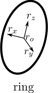
We have in total 4 Crazyflies and 1 Crazyradio for the communication between PC and Crazyflies. Since Crazyflies cannot directly communicate with each other, all communications were completed through PC. We used vicon system to track Crazyflies. On top of each Crazyflie, a infra-red led board is attached to strengthen the signal being observed by the vicon system. We used a hula loop to resemble a ring or opening. Three vicon markers were attached to the ring for tracking its position and orientation. The hardware used in this project are shown in Fig. 2.2.

2.3 Crazyflies Tracking

The vicon system outputs a set of unordered position measurements set $Z$ of which each element $z$ is the position measurement of a Crazyflie. Since the set is unordered, the correspondences of these measurements to the Crazyflies are unknown. In order to select the correct position measurement from the unordered measurements and be more robust to the missing measurements, we applied a kalman filter to track each Crazyflie. The Crazyflie is modelled as a random walk with unknown normally distributed acceleration $a_{i}$ . Assume the state vector of the Crazyflie $i$ is:

\displaystyle x_{i}=\begin{bmatrix}p_{i}\\ v_{i}\end{bmatrix}

(2.1)

Then the random walk model of the Crazyflie is:

	$\displaystyle p_{i}[k+1]$	$\displaystyle=p_{i}[k]+v_{i}[k]\delta t$		(2.2)
	$\displaystyle v_{i}[k+1]$	$\displaystyle=v_{i}[k]+a_{i}[k]$		(2.3)

where $\delta t=5$ ms is the time interval between two consecutive measurements of vicon system. We applied the standard kalman filter to estimate the state $x$ . Let $\hat{p}_{p,i}[k]$ and $\hat{v}_{p,i}[k]$ denote the prior updates of position and velocity of Crazyflie $i$ and $\hat{p}_{m,i}[k]$ and $\hat{v}_{m,i}[k]$ denote the measurement updates of Crazyflie $i$ . Then the prediction step at time $k$ for Crazyflie $i$ is:

	$\displaystyle\hat{p}_{p,i}[k+1]$	$\displaystyle=\hat{p}_{m,i}[k]+\hat{v}_{m,i}[k]\delta t$		(2.4)
	$\displaystyle\hat{v}_{p,i}[k+1]$	$\displaystyle=\hat{v}_{m,i}[k]$		(2.5)

Since only the positions are measured, the measurement model is:

$\displaystyle z_{i}$	$\displaystyle=H_{i}x_{i}+w_{i}$	(2.6)
	$\displaystyle=\begin{bmatrix}I&0\end{bmatrix}\begin{bmatrix}p_{i}\\ v_{i}\end{bmatrix}+w_{i}$	(2.7)
	$\displaystyle=p_{i}+w_{i}$	(2.8)

Before performing the measurement update step, the position measurement $z_{i}[k+1]$ of Crazyflie $i$ should be correctly picked from the unordered measurement set $Z$ . It is selected by searching a measurement $z$ that has the smallest euclidean distance to the predicted position $\hat{z}_{i}[k+1]=\hat{p}_{p,i}[k+1]$ :

\displaystyle z_{i}[k+1]=\underset{z\in Z}{\text{argmin}}\|z-\hat{z}_{i}[k+1]\|^{2}_{2}

(2.9)

and the measurement update step at time $k$ is:

	$\displaystyle\hat{p}_{m,i}[k+1]$	$\displaystyle=\hat{p}_{p,i}[k+1]+k_{p,i}(z_{i}[k+1]-\hat{z}_{i}[k+1])$		(2.10)
	$\displaystyle\hat{v}_{m,i}[k+1]$	$\displaystyle=\hat{v}_{p,i}[k+1]+k_{v,i}(z_{i}[k+1]-\hat{z}_{i}[k+1])$		(2.11)

where $k_{p,i}$ and $k_{v,i}$ are estimator gains. Thus we are able to track each Crazyflie from the unordered set of positions measurements. The tracked positions will be used for simulating the global position sensors and the bearing and distance sensor on Crazyflies.

2.4 Bearing and Distance Sensor

2.4.1 Sensor Simulation

As shown in Fig. 2.3 the bearing and distance sensor attached on the Crazyflie $i$ measures the distance and angle ${}_{i}z_{ji}(r,\theta,\phi)$ of Crazyflie $j$ in its local coordinate $\Sigma^{i}$ .

The local bearing and distance measurement ${}_{i}z_{ji}(r,\theta,\phi)$ is basically a Spherical coordinate representation. To simulate the bearing and distance sensor from vicon measurements, we first compute the global relative position measurement ${}_{g}z_{ji}$ from the tracked positions ${}_{g}z_{i}$ and ${}_{g}z_{j}$ .

{}_{g}z_{ji}=\text{${{}_{g}z_{j}}-{{}_{g}z_{i}}$}

(2.12)

and we can obtain the local representation of ${}_{g}z_{ji}$ in the local coordinate frame $\Sigma^{i}$ through the attitude matrix ${}_{ig}\hat{R}$ that is estimated by Crazyflie on-board attitude estimator:

{}_{i}z_{ji}={{}_{ig}\hat{R}^{-1}}_{g}z_{ji}

(2.13)

Let ${}_{i}z_{ji}=(x,y,z)$ , then the local bearing and distance measurement $(r,\theta,\phi)$ can be found as:

$\displaystyle r$	$\displaystyle=\sqrt{x^{2}+y^{2}+z^{2}}$	(2.14)
$\displaystyle\theta$	$\displaystyle=\arccos\frac{z}{\sqrt{x^{2}+y^{2}+z^{2}}}$	(2.15)
$\displaystyle\phi$	$\displaystyle=\arctan\frac{y}{x}$	(2.16)

2.4.2 Preprocessing of Sensor Measurements

To estimate the global position ${}_{g}p_{i}$ from the local bearing and distance ${}_{i}z_{ji}(r,\theta,\phi)$ of neighbor $j$ , a preprocessing step of transforming the Spherical representation to the global Cartesian representations is necessary. This transformation is illustrated in Fig. 2.4. For a distance and bearing measurement ${}_{i}z_{ji}(r,\theta,\phi)$ measured in Crazyflie $i$ ’s coordinate $\Sigma^{i}$ , we first transform it to the local Cartesian representation ${}_{i}z_{ji}(x,y,z)$ .

{}_{i}z_{ji}(x,y,z)=\prescript{}{i}{\begin{bmatrix}x\\ y\\ z\end{bmatrix}}=\begin{bmatrix}r\sin\theta\cos\phi\\ r\sin\theta\sin\phi\\ r\cos\theta\end{bmatrix}

(2.17)

Furthermore, the local Cartesian representation can also be transformed to the global Cartesian representation through the attitude matrix $\prescript{}{gi}{\hat{R}}$ .

{}_{g}z_{ji}(x,y,z)=\prescript{}{g}{\begin{bmatrix}x\\ y\\ z\end{bmatrix}}=\prescript{}{gi}{\hat{R}}\prescript{}{i}{\begin{bmatrix}x\\ y\\ z\end{bmatrix}}

(2.18)

With the global representation of relative position ${}_{g}z_{ji}(x,y,z)$ , the distributed observer is able to estimate the global positions of Crazyflies. Note that the attitude matrix $\prescript{}{gi}{\hat{R}}$ plays a crucial role here for the simulation and the preprocessing of the distance and bearing measurements.

2.5 Parameters

The parameters we used for tracking Crazyflie $i$ , $i\in 1,...,N$ when the discretization time step $\delta t=5$ ms are:

	$\displaystyle k_{p,i}=0.8$		(2.19)
	$\displaystyle k_{v,i}=0.0005$		(2.20)

Chapter 3 Distributed Observer

3.1 Observer Design

We assume that the underlying graph $G=(V,E)$ of the measurements is undirected and connected, that is, both Crazyflie $i$ and $j$ have the relative position measurement ${}_{g}z_{ij}$ , after the preprocessing step. Let the edge $(i,j)$ of $G$ be numbered with a unique $e\in\{1,...,m\}$ and consider all $N$ Crazyflies are modeled as double-integrators in $n$ -dimensional space (n=3):

\left\{\begin{array}[]{l}\dot{p}_{i}=v_{i},\\ \dot{v}_{i}=u_{i},\end{array}\right.,i=\{1,\ldots,N\}

(3.1)

The system dynamics in state space is:

\begin{bmatrix}\dot{p}\\ \dot{v}\end{bmatrix}=\underbrace{\begin{bmatrix}0&I_{nN}\\ 0&0\end{bmatrix}}_{\text{:=$A$}}\begin{bmatrix}p\\ v\end{bmatrix}+\underbrace{\begin{bmatrix}0\\ I_{nN}\end{bmatrix}}_{\text{:=$B$}}u

(3.2)

As discussed in the previous chapter, the relative measurements are represented in global Cartesian coordinate ${}_{g}z_{ji}(x,y,z)$ . From now on, the prescript $"g"$ and $(x,y,z)$ are dropped from ${}_{g}z_{ji}(x,y,z)$ for more concise notation.

We are able to express the relative measurements $z_{ij}$ and the global measurements $z_{i}$ through the incidence matrix $B$ and the selection matrix $E$ , where the selection matrix is defined as

\displaystyle E

\displaystyle=\begin{bmatrix}\cdots\underset{|}{\overset{|}{e_{i}}}\cdots\end{bmatrix},\quad i\in V_{g}

(3.3)

and $E^{T}z$ is a vector of all global measurements:

\displaystyle(E^{T}z)_{k}

\displaystyle=z_{i},\quad i\in V_{g}

(3.4)

where $V_{g}$ is the node list of Crazyflies that carry global position sensors. $e_{i}$ is the $i$ th column of the identity matrix $I_{N}$ . Let $x=[p^{T},v^{T}]^{T}$ and $\hat{x}=[\hat{p}^{T},\hat{v}^{T}]^{T}$ . Then we decompose all measurements into relative and absolute measurements as follows:

	$\displaystyle z$	$\displaystyle=Hx+w$		(3.5)
		$\displaystyle=\begin{bmatrix}B^{T}\otimes I_{n}&0\\ E^{T}\otimes I_{n}&0\end{bmatrix}\begin{bmatrix}p\\ v\end{bmatrix}+w$		(3.6)

The kronecker product $\otimes$ generalizes system to n-dimentional space and $w$ is the vector of measurement noise. A typical state observer can be designed as:

$\displaystyle\dot{\hat{x}}$	$\displaystyle=A\hat{x}+Bu+L(z-\hat{z})$	(3.7)
$\displaystyle\hat{z}$	$\displaystyle=H\hat{x}$	(3.8)
$\displaystyle z$	$\displaystyle=Hx+w$	(3.9)

Usually a steady state optimal kalman filter $K_{\infty}$ will be used to design the gain $L$ :

\dot{\hat{x}}=A\hat{x}+Bu+K_{\infty}(z-\hat{z})

(3.10)

However the optimal kalman gain $K_{\infty}$ is a dense matrix that will fuse all measurements $z$ available in the network to update each Crazyflie $i$ ’s state $\hat{x}_{i}$ [7]. This is not possible since the measurements and communications are only local and the local state observer of agent $i$ updates states only from the neighbors’ relative measurements and from its own global position measurements:

\displaystyle\begin{bmatrix}\dot{\hat{p}}_{i}\\ \dot{\hat{v}}_{i}\end{bmatrix}

\displaystyle=\begin{bmatrix}0&I_{n}\\ 0&0\end{bmatrix}\begin{bmatrix}\hat{p}_{i}\\ \hat{v}_{i}\end{bmatrix}+\begin{bmatrix}0\\ I_{n}\end{bmatrix}u_{i}+\left(\begin{bmatrix}k_{p}&k_{p}\\ k_{v}&k_{v}\end{bmatrix}\otimes I_{n}\right)\begin{bmatrix}\sum_{j\in N_{i}}k_{rp,ij}(z_{ij}-\hat{z}_{ij})\\ k_{gp,i}(z_{i}-\hat{z}_{i})\end{bmatrix}

(3.11)

where $k_{rp,i}>0$ and $k_{gp,i}\geq 0$ control the weights of the measurements available to $i$ and $k_{gp,i}=0$ if Crazyflie $i$ does not have global position measurement. $k_{p}$ and $k_{v}$ were used to fine-tune the gains for updating positions and velocities. Note that $\sum_{j\in N_{i}}$ only sums local weighted relative measurements error $k_{rp,i}(z_{ij}-\hat{z}_{ij})$ . As shown in Fig. 3.1(c), $(z_{ij}+\hat{z}_{j})$ can be viewed as a global position measurement of $i$ and its difference with the prediction of global position $\hat{z}_{i}$ is the measurement error:

\displaystyle z_{ij}+\hat{z}_{j}-\hat{z}_{i}=z_{ij}-\hat{z}_{ij}

(3.12)

Let $D_{rp}=\text{diag}(\{k_{rp,e}\})_{e\in{1,...,m}}$ , then $BD_{rp}B^{T}$ is a Laplacian matrix and

\displaystyle(BD_{rp}B^{T}(z-\hat{z}))_{i}=\sum_{j\in N_{i}}k_{rp,ij}(z_{ij}-\hat{z}_{ij})

(3.13)

Let $D_{gp}=\text{diag}(\{k_{gp,i}\})_{i\in V_{g}}$ , then

\displaystyle(ED_{gp}E^{T}(z-\hat{z}))_{i}=k_{gp,i}(z_{i}-\hat{z}_{i})

(3.14)

Therefore the distributed observer can be written in a compact form as:

\displaystyle\begin{bmatrix}\dot{\hat{p}}\\ \dot{\hat{v}}\end{bmatrix}

\displaystyle=\begin{bmatrix}0&I_{nN}\\ 0&0\end{bmatrix}\begin{bmatrix}\hat{p}\\ \hat{v}\end{bmatrix}+\begin{bmatrix}0\\ I_{nN}\end{bmatrix}u+L_{1}H\begin{bmatrix}z-\hat{z}\end{bmatrix}

(3.15)

and the observer gain $L_{1}$ is:

\displaystyle L_{1}

\displaystyle=\begin{bmatrix}k_{p}BD_{rp}&k_{p}ED_{gp}\\ k_{v}BD_{rp}&k_{v}ED_{gp}\end{bmatrix}\otimes I_{n}

(3.16)

3.2 Stability

To study the stability of above observer, let $e=[p^{T},v^{T}]^{T}-[\hat{p}^{T},\hat{v}^{T}]^{T}$ . Then

\dot{e}=\underbrace{(A-L_{1}H)}_{\text{:=$\mathcal{O}$}}e

(3.17)

and

$\displaystyle\mathcal{O}=A-L_{1}H$	$\displaystyle=\begin{bmatrix}0&I_{nN}\\ 0&0\end{bmatrix}-\begin{bmatrix}k_{p}BD_{rp}&k_{p}ED_{ap}\\ k_{v}BD_{rp}&k_{v}ED_{ap}\end{bmatrix}\otimes I_{n}\begin{bmatrix}B^{T}&0\\ E^{T}&0\end{bmatrix}\otimes I_{n}$	(3.18)
	$\displaystyle=\begin{bmatrix}0&I_{nN}\\ 0&0\end{bmatrix}-\begin{bmatrix}k_{p}BD_{rp}B^{T}+k_{p}ED_{ap}E^{T}&0\\ k_{v}BD_{rp}B^{T}+k_{v}ED_{ap}E^{T}&0\end{bmatrix}\otimes I_{n}$	(3.19)
	$\displaystyle=\underbrace{\begin{bmatrix}-k_{p}BD_{rp}B^{T}-k_{p}ED_{ap}E^{T}&I_{N}\\ -k_{v}BD_{rp}B^{T}-k_{v}ED_{ap}E^{T}&0\end{bmatrix}}_{:=\mathcal{O^{\prime}}}\otimes I_{n}$	(3.20)

To ensure the observer estimates states properly, the error dynamics matrix $\mathcal{O}$ needs to be asymptotically stable. The kronecker product only add multiplicities of each eigenvalues and do not affect stability. We then find eigenvalues of $\mathcal{O^{\prime}}$ to study the stability of $\mathcal{O}$ by solving $det(\lambda I_{2N}-\mathcal{O^{\prime}})=0$ .

$\displaystyle det(\lambda I_{2N}-\mathcal{O^{\prime}})$	$\displaystyle=det(\begin{bmatrix}\lambda I_{N}&0\\ 0&\lambda I_{N}\end{bmatrix}-\begin{bmatrix}-k_{p}BD_{rp}B^{T}-k_{p}ED_{ap}E^{T}&I_{N}\\ -k_{v}BD_{rp}B^{T}-k_{v}ED_{ap}E^{T}&0\end{bmatrix})$	(3.21)
	$\displaystyle=det(\begin{bmatrix}\lambda I_{N}+k_{p}BD_{rp}B^{T}+k_{p}ED_{ap}E^{T}&-I_{N}\\ k_{v}BD_{rp}B^{T}+k_{v}ED_{ap}E^{T}&\lambda I_{N}\end{bmatrix})$	(3.22)
	$\displaystyle=det(\lambda^{2}I_{N}+\lambda k_{p}BD_{rp}B^{T}+\lambda k_{p}ED_{ap}E^{T}+k_{v}BD_{rp}B^{T}+k_{v}ED_{ap}E^{T})$	(3.23)
	$\displaystyle=det(\lambda^{2}I_{N}+(\lambda k_{p}+k_{v})(\underbrace{BD_{rp}B^{T}+ED_{ap}E^{T}}_{\text{$:=\mathcal{T}$}}))$	(3.24)

Let $\mu_{i}$ be $i$ th eigenvalue of $\mathcal{T}$ , then

\displaystyle det(\lambda^{2}I_{N}+(\lambda k_{p}+k_{v})\mathcal{T})=\prod_{i}^{N}(\lambda^{2}+(\lambda k_{p}+k_{v})\mu_{i})=0

(3.25)

Then we can solve above equation to find $\lambda$

\displaystyle\lambda^{2}+(\lambda k_{p}+k_{v})\mu_{i}=0

(3.26)

The Routh-Hurwitz stability criterion tells us that if the coefficients of second order polynomial are all positive then the roots are in the left half plane. Therefore if $\mu_{i}>0$ , then $\mathcal{O^{\prime}}$ is Hurwitz. It is easy to verify that $\mathcal{T}$ is positive definite and thus $\mu_{i}>0$ :

$\displaystyle x^{T}\mathcal{T}x$	$\displaystyle=x^{T}(BD_{rp}B^{T}+ED_{ap}E^{T})x$	(3.27)
	$\displaystyle=\\|\sqrt{D_{rp}}B^{T}x\\|^{2}_{2}+\\|\sqrt{D_{ap}}E^{T}x\\|^{2}_{2}$	(3.28)
	$\displaystyle\geq 0,\quad\forall x\in R^{3N}$	(3.29)

Since $\|\sqrt{D_{rp}}B^{T}x\|=0$ if and only if $x=\beta\mathbf{1}_{3N}=\beta(1,,,1)$ , $\beta\in\Re$ and $\|E^{T}(\beta\mathbf{1}_{3N})\|>0$ ,

\displaystyle x^{T}\mathcal{T}x

\displaystyle=\|\sqrt{D_{rp}}B^{T}x\|^{2}_{2}+\|\sqrt{D_{ap}}E^{T}x\|^{2}_{2}>0,\quad\forall x\in R^{3N}

(3.30)

Thus $\mu_{i}>0$ and $\mathcal{O^{\prime}}$ is Hurwitz. The estimation error $\tilde{e}=[p^{T},v^{T}]^{T}-[\hat{p}^{T},\hat{v}^{T}]^{T}$ will asymptotically converge to zero. Thus all the agents are able to estimate positions and velocities, and we are ready to apply distributed control law to control the swarm.

3.3 Parameters

The observer gains to update position and velocity are:

	$\displaystyle k_{p}=0.8$		(3.31)
	$\displaystyle k_{v}=20.0$		(3.32)

(a) If i measures global position, the observer gains used in this project are:

	$\displaystyle k_{rp,ij}=k_{gp,i}=\frac{k_{p}}{N_{i}+1},\quad\forall i\in V_{g}$		(3.33)
	$\displaystyle k_{rv,ij}=k_{gv,i}=\frac{k_{v}}{N_{i}+1},\quad\forall i\in V_{g}$		(3.34)

(b) If i has no global position sensor $i\in V\setminus V_{g}$ , then:

	$\displaystyle k_{rp,ij}=\frac{k_{p}}{N_{i}}$		(3.35)
	$\displaystyle k_{gp,i}=0$		(3.36)
	$\displaystyle k_{rv,ij}=\frac{k_{v}}{N_{i}}$		(3.37)
	$\displaystyle k_{gv,i}=0$		(3.38)

The parameters selected may not be optimal and need to be further tuned by trial and error in practice.

Chapter 4 Distributed Control

4.1 Controller Design

Let $p^{*}=[...,p^{*T}_{i},...]^{T}$ and $v^{*}=[...,v^{*T}_{i},...]^{T}$ be the desired global positions and velocities of all Crazyflies. Then the desired relative positions and velocities between $i$ and $j$ are $p^{*}_{ij}=p^{*}_{i}-p^{*}_{j}$ and $v^{*}_{ij}=v^{*}_{i}-v^{*}_{j}$ . Among the Crazyflies, leaders are able to control the global positions $p^{*}_{i}$ and velocities $v^{*}_{i}$ , whereas followers can only control the relative positions $p^{*}_{ij}$ and velocities $v^{*}_{ij}$ . To maintain the formation, we propose implementing following formation control law on each Crazyflie $i$ [10]:

$\displaystyle u_{i}=$	$\displaystyle\quad u_{rp,i}+u_{rv,i}+u_{gp,i}+u_{gv,i}$	(4.1)
$\displaystyle u_{i}=$	$\displaystyle-\sum_{j\in N_{i}}k_{rp,ij}(p_{i}-p_{j}-p^{*}_{ij})$	(4.2)
	$\displaystyle-\sum_{j\in N_{i}}k_{rv,ij}(v_{i}-v_{j}-v^{*}_{ij})$	(4.3)
	$\displaystyle-k_{gp,i}(p_{i}-p_{i}^{*})$	(4.4)
	$\displaystyle-k_{gv,i}(v_{i}-v_{i}^{*})$	(4.5)

where $u_{rp,i}$ controls relative positions to achieve the desired formations, $u_{rv,i}$ controls relative velocities for the flocking behavior of the swarm, $u_{gp,i}$ controls the global position of the swarm, and $u_{gv,i}$ controls global velocity of the swarm. In addition, $k_{rp,ij}>0$ , $k_{rv,ij}>0$ are the control gains for relative positions and velocities to neighbors. $k_{gp,i}\geq 0$ , $k_{gv,i}\geq 0$ are control gains for the global positions and velocities. Only when Crazyflie $i$ is a leader, $k_{gp,i}>0$ , $k_{gv,i}>0$ .

We assume the underlying graph to control positions and velocities be $G_{rp}=(V,E,\{k_{rp,e}\}_{e\in E})$ and $G_{rv}=(V,E,\{k_{rv,e}\}_{e\in E})$ respectively, which are both undirected and connected. Let $L_{p}$ and $L_{v}$ denote the Laplacian matrices for these two graphs. Let $G_{p}$ and $G_{v}$ be defined element-wise as:

	$\displaystyle(G_{p}x)_{i}=k_{gp,i}x_{i}$		(4.6)
	$\displaystyle(G_{v}x)_{i}=k_{gv,i}x_{i}$		(4.7)

and assume the ratio of control gains of position to velocity is constant $\alpha$ , $\alpha\in\Re$ :

	$\displaystyle k_{gp,i}$	$\displaystyle=\alpha k_{gv,i}$		(4.8)
	$\displaystyle k_{rp,ij}$	$\displaystyle=\alpha k_{rv,ij}$		(4.9)

Then the distributed control law in a compact form is:

$\displaystyle u$	$\displaystyle=K(x-x^{*})$	(4.10)
	$\displaystyle=\begin{bmatrix}-(L_{p}\otimes I_{n})-(G_{p}\otimes I_{n})&-(L_{v}\otimes I_{n})-(G_{v}\otimes I_{n})\end{bmatrix}\begin{bmatrix}p-p^{}\\ v-v^{}\end{bmatrix}$	(4.11)
	$\displaystyle=\begin{bmatrix}-(\alpha L_{v}\otimes I_{n})-(\alpha G_{v}\otimes I_{n})&-(L_{v}\otimes I_{n})-(G_{v}\otimes I_{n})\end{bmatrix}\begin{bmatrix}p-p^{}\\ v-v^{}\end{bmatrix}$	(4.12)

and we obtain the closed loop dynamics:

$\displaystyle\dot{x}$	$\displaystyle=Ax+Bu$	(4.13)
$\displaystyle\dot{x}$	$\displaystyle=Ax+BK(x-x^{*})$	(4.14)
$\displaystyle\dot{x}^{*}-\dot{x}$	$\displaystyle=\dot{x}^{}-Ax-BK(x-x^{})$	(4.15)
$\displaystyle\dot{x}^{*}-\dot{x}$	$\displaystyle=\dot{x}^{}-A(x-x^{}+x^{})-BK(x-x^{})$	(4.16)
$\displaystyle\dot{x}^{*}-\dot{x}$	$\displaystyle=\dot{x}^{}-Ax^{}-A(x-x^{})-BK(x-x^{})$	(4.17)
$\displaystyle\dot{x}^{*}-\dot{x}$	$\displaystyle=Bu^{}-(A+BK)(x-x^{})$	(4.18)

Let $e=x^{*}-x$ , $e_{p}=p^{*}-p$ and $e_{v}=v^{*}-v$ , we then obtain the following error dynamics

$\displaystyle\dot{e}$	$\displaystyle=(A+BK)e+Bu^{*}$	(4.19)
$\displaystyle\begin{bmatrix}\dot{e}_{p}\\ \dot{e}_{v}\end{bmatrix}$	$\displaystyle=\underbrace{\begin{bmatrix}0&I_{nN}\\ -(\alpha L_{v}\otimes I_{n})-(\alpha G_{v}\otimes I_{n})&-(L_{v}\otimes I_{n})-(G_{v}\otimes I_{n})\end{bmatrix}}_{\text{$:=\mathcal{M}$}}\begin{bmatrix}e_{p}\\ e_{v}\end{bmatrix}+Bu^{*}$	(4.20)
	$\displaystyle=\left(\underbrace{\begin{bmatrix}0&I_{N}\\ -(\alpha L_{v}+\alpha G_{v})&-(L_{v}+G_{v})\end{bmatrix}}_{:=\mathcal{M}^{\prime}}\otimes I_{n}\right)\begin{bmatrix}e_{p}\\ e_{v}\end{bmatrix}+Bu^{*}$	(4.21)

One must make sure $\mathcal{M}^{\prime}$ is Hurwitz such that $e_{p}$ and $e_{v}$ are bounded given $u^{*}$ is bounded. $u^{*}$ is the desired feed-forward input which is unknown.

4.2 Stability

Similar to the observer, we compute the eigenvalues of $\mathcal{M}^{\prime}$ to test its stability:

$\displaystyle det(\lambda I_{2N}-\mathcal{M}^{\prime})$	$\displaystyle=det(\begin{bmatrix}\lambda I_{N}&0\\ 0&\lambda I_{N}\end{bmatrix}-\begin{bmatrix}0&I_{N}\\ -(\alpha L_{v}+\alpha G_{v})&-(L_{v}+G_{v})\end{bmatrix})$	(4.22)
	$\displaystyle=det(\begin{bmatrix}\lambda I_{N}&-I_{N}\\ \alpha L_{v}+\alpha G_{v}&\lambda I_{N}+L_{v}+G_{v}\end{bmatrix})$	(4.23)
	$\displaystyle=det(\lambda^{2}I_{N}+\lambda L_{v}+\lambda G_{v}+\alpha L_{v}+\alpha G_{v})$	(4.24)
	$\displaystyle=det(\lambda^{2}I_{N}+(\lambda+\alpha)L_{v}+(\lambda+\alpha)G_{v})$	(4.25)
	$\displaystyle=det(\lambda^{2}I_{N}+(\lambda+\alpha)(\underbrace{L_{v}+G_{v}}_{:=\Gamma}))$	(4.26)

Let $\gamma_{i}$ be the $i$ th eigenvalue of $\Gamma$ , then

\displaystyle det(\lambda^{2}I_{N}+(\lambda+\alpha)\Gamma)

\displaystyle=\prod^{N}_{i}(\lambda^{2}+(\lambda+\alpha)\gamma_{i})=0

(4.27)

Again if $\gamma_{i}>0$ then $Re\{\lambda\}<0$ .

$\displaystyle x^{T}(L_{v}+G_{v})x$	$\displaystyle=x^{T}(L_{v}+G_{v})x$	(4.28)
	$\displaystyle=x^{T}L_{v}x+x^{T}G_{v}x$	(4.29)
	$\displaystyle\geq 0$	(4.30)

where $x^{T}L_{v}x\geq 0$ since $L_{v}$ is a Laplacian matrix which has non-negative eigenvalues and $L_{v}x=0$ if and only if $x=\beta\mathbf{1}_{N}$ , $\beta\in\Re$ . $x^{T}G_{v}x\geq 0$ because $G_{v}$ is a diagonal matrix with non-negative diagonal. Since $x^{T}G_{v}x>0$ when $x=\beta\mathbf{1}_{N}$ ,

\displaystyle x^{T}(L_{v}+G_{v})x=x^{T}L_{v}x+x^{T}G_{v}x>0

(4.31)

Thus $\gamma_{i}>0$ and the eigenvalue $\lambda$ of $\mathcal{M}$ has negative real part. The error dynamics matrix $\mathcal{M}$ is asymptotically stable.

4.3 Parameters

If $i$ is a leader $i\in V_{g}$ , the control gains for position and velocity are:

	$\displaystyle k_{gp,i}=\frac{9.0}{N_{i}+1}$		(4.32)
	$\displaystyle k_{gv,i}=\frac{4.0}{N_{i}+1}$		(4.33)
	$\displaystyle k_{rp,ij}=\frac{9.0}{N_{i}+1}$		(4.34)
	$\displaystyle k_{rv,ij}=\frac{4.0}{N_{i}+1}$		(4.35)

If $i$ is a follower $i\in V\setminus V_{g}$ ,

	$\displaystyle k_{gp,i}=0$		(4.36)
	$\displaystyle k_{gv,i}=0$		(4.37)
	$\displaystyle k_{rp,ij}=\frac{9.0}{N_{i}}$		(4.38)
	$\displaystyle k_{rv,ij}=\frac{4.0}{N_{i}}$		(4.39)

Basically the above parameters mean that the relative position and velocity error to the neighbors are averaged to generate the final control output. This is simple and but may not be optimal. In practice they should be fine-tuned by trial and error.

4.4 Discussion

The distributed control in this project is only suitable for maintaining formations in free space. The collision avoidance was not considered in designing the control law. In literature, Lyapunov functions with infinite potential energy were often proposed to achieve collision avoidance [11]. This is not realistic as physical systems have limited amount of actuation. This motivates us to apply optimization based trajectory generation to deal with complex environments and constraints as will be discussed in chapter 6.

Chapter 5 Formation Scale Estimation

5.1 Estimator Design

The distributed control maintains a constant shape of the formation by controlling the relative positions and velocities. Crazyflies need to know the scale factor of the relative positions and velocities to change the formation scale. In this chapter we discuss how to estimate the scale of the formation.

Assume the center of the formation is $(p^{c},v^{c})$ and the desired relative position and velocities are $(p^{r},v^{r})$ with zero mean, i.e., $\sum_{e\in{1,...,m}}p^{r}_{e}=0$ and $\sum_{e\in{1,...,m}}v^{r}_{e}=0$ . Then we are able to write the desired trajectories of the system as:

\displaystyle\begin{bmatrix}p^{*}\\ v^{*}\end{bmatrix}=\begin{bmatrix}p^{c}\\ v^{c}\end{bmatrix}+\begin{bmatrix}p^{r}\\ v^{r}\end{bmatrix}

(5.1)

and

\displaystyle v^{r}=\dot{p}^{r}

(5.2)

Sometimes the desired scale of the formation change over time, for example, to avoid collisions. Then the desired relative positions and velocities are not constant anymore and the desired trajectories can be rewritten as:

	$\displaystyle\begin{bmatrix}p^{}\\ v^{}\end{bmatrix}$	$\displaystyle=\begin{bmatrix}p^{c}\\ v^{c}\end{bmatrix}+\begin{bmatrix}p^{r}\\ \dot{p}^{r}\end{bmatrix}$		(5.3)
		$\displaystyle=\begin{bmatrix}p^{c}\\ v^{c}\end{bmatrix}+\begin{bmatrix}s(t)\bar{p}^{r}\\ \dot{s}(t)\bar{p}^{r}\end{bmatrix}$		(5.4)

where $s(t)>0$ is the time varying scale and $\bar{p}^{r}$ is the relative positions when $s(t)=1$ . Since we only allow leaders to have the information of the desired scale $s(t)$ , the followers must communicate with neighbors to obtain this scale. One approach is that the scale $s(t)$ can be transmitted by leaders to their neighbors who in turn transmit $s(t)$ to their neighbors [4]. However each follower needs to know among which of its neighbors there is a path to the leaders. This may not be robust in case the roles of leaders and followers may change and the communication may be lost. A better solution is again using distributed law to fuse all neighbors’ information to estimate the scale regardless of the path to leaders [4]. Assume the underlying communication graph $G$ is undirected and connected with weights $a_{ij}$ and $L_{s}$ is its Laplacian matrix. Let $V_{g}$ be the list of leaders who know the desired scale $s(t)$ and $s_{est,i}=[...,s_{est,i},...]^{T}$ be the scale estimate vector of all Crazyflies. The Crazyflie $i$ updates $s_{est,i}$ through:

\displaystyle\dot{s}_{est,i}=-\sum_{j\in N_{i}}a_{ij}(s_{est,i}-s_{est,j})-g_{i}(s_{est,i}-s(t))

(5.5)

and

\displaystyle\left\{\begin{aligned} g_{i}&=g>0,\quad\text{if}\ i\in V_{g}\\ g_{i}&=0,\quad\text{otherwise}\end{aligned}\right.

(5.6)

Let $G_{s}$ be a diagonal matrix and

\displaystyle(G_{s})_{i}=g,\quad i\in V_{g}

(5.7)

Then we can write the estimation dynamics in compact form:

\displaystyle\dot{s}_{est}=-L_{s}s_{est}-G_{s}(s_{est}-s\mathbf{1}_{N})

(5.8)

5.2 Stability

Let $e:=s_{est}-s\mathbf{1}_{N}$ . If $s(t)$ is varying slowly and $\dot{s}(t)$ is bounded the estimation error $e(t)$ is bounded from the bounded input bounded state theory:

$\displaystyle\dot{s}_{est}-\dot{s}\mathbf{1}_{N}$	$\displaystyle=-L_{s}s_{est}-G_{s}(s_{est}-s\mathbf{1}_{N})-\dot{s}\mathbf{1}_{N}$	(5.9)
$\displaystyle\dot{e}$	$\displaystyle=-(L_{s}+G_{s})(s_{est}-s\mathbf{1}_{N})-\dot{s}\mathbf{1}_{N},\quad\textrm{since }L_{s}\mathbf{1}_{N}=0_{N}$	(5.10)
$\displaystyle\dot{e}$	$\displaystyle=-(L_{s}+G_{s})e-\dot{s}\mathbf{1}_{N}$	(5.11)

As before, $x^{T}L_{s}x\geq 0$ and $x^{T}L_{s}x=0$ if and only if $x=\beta\mathbf{1}_{N}$ , $\beta\in\Re$ and $\mathbf{1}_{N}^{T}G_{s}\mathbf{1}_{N}>0$ . Therefore $L_{s}+G_{s}$ is exponentially stable.

Note that $\dot{p}^{*}=v^{*}$ and $\dot{p}^{c}=v^{c}$ . Then

	$\displaystyle p^{*}$	$\displaystyle=p^{c}+s(t)\bar{p}^{r}$		(5.12)
	$\displaystyle v^{*}$	$\displaystyle=\dot{p}^{c}+\dot{s}(t)\bar{p}^{r}$		(5.13)

Substitute $s(t)$ and $\dot{s}(t)$ with the estimated scale $s_{est}$ and $\dot{s}_{est}$ , we obtain

	$\displaystyle p^{*}_{est}$	$\displaystyle\approx p^{c}+(\textrm{diag}(s_{est})\otimes I_{n})\bar{p}^{r}$		(5.14)
	$\displaystyle v^{*}_{est}$	$\displaystyle\approx\dot{p}^{c}+(\textrm{diag}(\dot{s}_{est})\otimes I_{n})\bar{p}^{r}$		(5.15)

Then we are able to write the approximated desired trajectories as:

\displaystyle\begin{bmatrix}p^{*}_{est}\\ v^{*}_{est}\end{bmatrix}\approx\begin{bmatrix}p^{c}\\ v^{c}\end{bmatrix}+\begin{bmatrix}\textrm{diag}(s_{est})\otimes I_{n}\\ \textrm{diag}(-(L_{s}+G_{s})s_{est}+sG_{s}\textbf{1}_{N})\otimes I_{n}\end{bmatrix}\bar{p}^{r}

(5.16)

Thus the approximated desired relative positions and velocities are obtained from the estimated scale factor $s_{est}$ . Crazyflies then can apply the formation control law to maintain the estimated time varying desired relative positions and velocities.

5.3 Parameters

We again average neighbors’ estimates $s_{est,j}$ , $j\in N_{i}$ to update $s_{est,i}$ :

(a) If $i$ is a leader, $i\in V_{g}$ , then

\displaystyle a_{ij}=g_{i}=\frac{1}{N_{i}+1}

(5.17)

(b) If $i$ is a follower, $i\in V\setminus V_{g}$ , then

	$\displaystyle a_{ij}=\frac{1}{N_{i}}$		(5.18)
	$\displaystyle g_{ij}=0$		(5.19)

Chapter 6 Distributed Trajectory Optimization

6.1 Centralized Trajectory Optimization

Federico proposed a discrete time trajectory optimization method to compute collision-free trajectories in a centralized manner [1]. The optimization problem is:

(6.3)

where $x\in\Re^{3NK}$ is the stacked acceleration vectors of all quadcopters. Let $T$ and $k$ denote the trajectory duration and discretization time step, then $K=\frac{T}{h}$ . The equality constraint $A_{eq}=b_{eq}$ represents initial and final positions and velocities of the quadcopters and the inequality constraint $A_{in}x\preceq b_{in}$ contains the convexified collision avoidance constraints and other physical constraints, e.g., actuator constraints. Since the jerks of quadcopter is related to the magnitude of body rates, we seek for a minimum jerk solution to reduce the aggressiveness of attitude changing during the flight [9]:

(6.6)

where $D$ is to compute forward difference of $x$ to approximate the derivative of acceleration $x$ . The above centralized approach scales poorly with number of Crazyflies. There are $O(N^{2})$ collision avoidance constraints and $O(N)$ optimization variables. In the following sections we discuss how to make the optimization more scalable.

6.2 Initial Solution

To obtain the convexified collision avoidance constraints and the ring constraint $A_{in}x\preceq b_{in}$ , we need either an initial guess or a previous solution. Here we discuss one possible solution as the initial guess.

We first solve the optimization problem 6.6 without $A_{in}\preceq b_{in}$ to find a straight line solution for each Crazyflie without considering the collision avoidance and ring constraints, which is shown in figure 6.1

The straight line solution is used for finding a proper crossing time $k_{c}$ to impose the ring constraint. Then a velocity constraint at the position of the crossing time is imposed and the initial solution is refined such that it passes through the center of ring perpendicularly with a reasonable speed.

6.3 Collision Avoidance Constraints

There are two types of collisions considered to solve the optimization problem 6.6:

6.3.1 Collisions between Crazyflie and ring

The ring resembles an opening that only its interior is allowed to pass through as illustrated in Fig. 6.3. Therefore, Crazyflie should avoid hitting on or bypassing the ring. The ring object can be modelled as a convex circle constraint if we know the time to impose it when the Crazyflie crosses the ring. However it is unknown before solving the optimization problem. The following steps estimate a crossing time and convexify the ring constraint using an initial or previous $q$ th solution $p^{q}_{i}[k]$ :

1.

find $k^{i}_{c}=\underset{k\in 1,...,K}{\text{argmin}}\|p^{q}_{i}[k]-r_{o}\|^{2}_{2}$
2.

let $p^{q+1}_{i}[k^{i}_{c}]\in tube$
3.

let $p^{q+1}_{i}[k^{i}_{c}-1]\in leftCone$
4.

let $p^{q+1}_{i}[k^{i}_{c}+1]\in rightCone$

We used a tube and two cones to approximate the ring constraint such that Crazyflie will avoid collisions before and after passing through it. The reason for imposing only two cone constraints is that it makes the constraints only be local near the ring and will not affect the optimization of trajectory far from the ring. This on one hand limits the number of constraints and on the other hand it also reduces the chances of infeasibility when the initial or final position that cannot be optimized are not within the cone, which results in an infeasible problem.

tube

	$\displaystyle\left\|{r}_{y}^{T}(p^{q+1}_{i}[k^{i}_{c}]-r_{o})\right\|\leq R_{tube}$		(6.7)
	$\displaystyle\left\|{r}_{z}^{T}(p^{q+1}_{i}[k^{i}_{c}]-r_{o})\right\|\leq R_{tube}$		(6.8)

leftCone

	$\displaystyle\left\|{r}_{y}^{T}(p^{q+1}_{i}[k^{i}_{c}-1]-r_{o})\right\|\leq{r}_{x}^{T}(p^{q+1}_{i}[k^{i}_{c}-1]-r_{o})$		(6.9)
	$\displaystyle\left\|{r}_{z}^{T}(p^{q+1}_{i}[k_{c}-1]-r_{o})\right\|\leq{r}_{x}^{T}(p^{q+1}_{i}[k^{i}_{c}-1]-r_{o})$		(6.10)

rightCone

	$\displaystyle\left\|{r}_{y}^{T}(p^{q+1}_{i}[k^{i}_{c}+1]-r_{o})\right\|\leq-{r}_{x}^{T}(p^{q+1}_{i}[k^{i}_{c}+1]-r_{o})$		(6.11)
	$\displaystyle\left\|{r}_{z}^{T}(p^{q+1}_{i}[k^{i}_{c}+1]+r_{o})\right\|\leq-{r}_{x}^{T}(p^{q+1}_{i}[k^{i}_{c}+1]-r_{o})$		(6.12)

6.3.2 Collisions between Crazyflies

To avoid collisions between Crazyflies themselves at each $k$ , a safe distance margin $R_{collision}=0.3$ m between Crazyflies’ centers is enforced. This margin is large enough to tolerate certain control error when Crazyflies are tracking the trajectories. The collision avoidance constraint between Crazyflies $i$ and $j$ at time $k$ is a non-convex constraint:

\displaystyle\|p_{i}[k]-p_{j}[k]\|_{2}\geq R_{collision}\quad\forall i,j\in 1,...,N,\ i\neq j

(6.13)

To convexify this constraint, again we need an initial guess or previous solution $p^{q}_{i}[k],p^{q}_{j}[k]$ . Assume the new solutions are $p^{q+1}_{i}$ and $p^{q+1}_{j}$ , then the convexified constraint is [1]:

\displaystyle\eta^{T}(p^{q+1}_{i}[k]-p^{q+1}_{j}[k])\geq R_{collision},\quad\eta=\frac{p^{q}_{i}[k]-p^{q}_{j}[k]}{\|p^{q}_{i}[k]-p^{q}_{j}[k]\|_{2}}

(6.14)

Note that this convexified constraint assumes the optimization variables are $p^{q+1}_{i}[k],p^{q+1}_{j}[k]$ . We can also optimize only $p^{q+1}_{i}[k]$ for Crazyflie $i$ and $p^{q+1}_{j}[k]$ for Crazyflie $j$ independently [3].

	$\displaystyle\eta^{T}(p^{q+1}_{i}[k]-p^{q}_{j}[k])\geq R_{collision},\quad\eta=\frac{p^{q}_{i}[k]-p^{q}_{j}[k]}{\\|p^{q}_{i}[k]-p^{q}_{j}[k]\\|_{2}}$		(6.15)
	$\displaystyle\eta^{T}(p^{q}_{i}[k]-p^{q+1}_{j}[k])\geq R_{collision},\quad\eta=\frac{p^{q}_{i}[k]-p^{q}_{j}[k]}{\\|p^{q}_{i}[k]-p^{q}_{j}[k]\\|_{2}}$		(6.16)

As shown in Fig. 6.5, the convexified constraints Eqn. 6.14 and Eqn. 6.15 are different. Eqn. 6.14 is a relative constraint that the infeasible region can move along the direction of $\eta$ , whereas Eqn. 6.14 is an absolute constraint that the infeasible region is static. Clearly the collision constraints convexified with Eqn. 6.14 have larger feasible regions.

6.4 Distributed Constrained Convex Optimization

After discussing constructing initial solution and convexfication of collision constraints, we begin discussing the method to make the optimization problem more scalable. Recently there is an increasing interest in enabling agents to cooperatively solve the following distributed constrained convex optimization:

(6.19)

where each $f_{i}$ is a local objective function and $X_{i}$ is a local feasible set. The important observation here is that both the objective function $f_{0}$ and constraint set $X$ are decomposed as individual local objective functions and feasible sets. The distributed projected subgradient algorithm to solve the above problem is [6]:

\displaystyle x_{i}(m+1)=P_{X_{i}}\left[\sum_{j\in N_{i}\cup i}a_{ij}x_{j}(m)-\alpha_{m}d_{i}(m)\right]

(6.20)

where $x_{i}(m)\in\Re^{3NK}$ is the local estimate of $x$ at time m, $a_{ij}$ is an entry of adjacency matrix $A$ of the underlying communication graph $G$ , $\alpha_{m}>0$ is the step size of subgradient algorithm at time $m$ , and $d_{i}(m)$ is a subgradient of local objective function at $\sum_{j\in N_{i}\cup i}a_{ij}x_{j}(m)$ . $P_{X_{i}}[x]$ is the projection of $x$ onto $X_{i}$ , i.e. $P_{X_{i}}(x)=\textrm{argmin}_{\bar{x}\in X_{i}}\|\bar{x}-x\|$ . The distributed projected subgradient algorithm converges as $m\rightarrow\infty$ :

\displaystyle\lim_{m\rightarrow\infty}\|x_{i}(m)-x_{j}(m)\|^{2}_{2}=0

(6.21)

under the following assumptions [6]:

1.

$X$ is nonempty and has nonempty interior.
2.

The graph $G$ is fixed and strongly connected.
3.

$a_{ij}>\eta$ , $0<\eta<1$ .
4.

$A$ is doubly stochastic.
5.

$X$ is compact.
6.

$\sum^{+\infty}_{m=0}\alpha_{m}=+\infty$ and $\sum^{+\infty}_{m=0}\alpha^{2}_{m}<\infty$

Remark 1.

The $x_{i}(m)$ is a local estimate of $x$ at time m. The termination condition of the algorithm is that all the local estimates converge sufficiently close to each other, i.e., $\|x_{i}(m)-x_{j}(m)\|^{2}_{2}<\epsilon$ , and we may assume at most $M$ iterations the algorithm can converge.

Remark 2.

There are three operations involved in this algorithm. (a) $\sum_{j\in N_{i}\cup i}a_{ij}x_{j}(m)$ is a standard distributed averaging step such that $x_{i}(m)$ and $x_{j}(m)$ reach consensus as $m\rightarrow\infty$ . (b) $-\alpha_{m}d_{i}(m)$ is a subgradient step to reduce the local objective function value. (c) $P_{X_{i}}[x]$ projects the averaged and subgradient subtracted solution to the local feasible set $X_{i}$ . The combined three steps allows the local solution $x_{i}(m)$ to reach consensus with neighbors asymptotically as $m\rightarrow\infty$ and cooperatively reduce the value of objective function $f_{0}=\sum^{N}_{i=1}f_{i}(x)$ while satisfying their own local constraint $X_{i}$ after the projection $P_{X_{i}}[x]$ .

In order to solve Problem 6.6, we express it in the form of problem 6.19 as:

(6.24)

where $D_{i}$ computes the jerk of Crazyflie $i$ , $A_{eq}\ x=b_{eq}$ is the initial to final state condition of all Crazyflies, and $A_{in,i}\ x\preceq b_{in,i}$ includes the convexified collision avoidance constraints of Crazyflie $i$ with the remaining $N-1$ Crazyflies and other constraints local to $i$ , e.g., $a_{min,i}\preceq x_{i}\preceq a_{max,i}$ .

Remark 3.

The assumption 1 that $X$ has nonempty interior does not strictly hold for problem 6.24 as the equality constraint $A_{eq}\ x=b_{eq}$ is present. However experiments show that the algorithm still converges. One reason may be that all the Crazyflies share the same equality constraint $A_{eq}\ x=b_{eq}$ , which does not affect the convergence of algorithm that assumes only inequality constraints exist. The assumption 3 and 4 can be guaranteed by setting $a_{ij}=\frac{1}{N_{i}+1}$ , which also simplifies the algorithm design. The assumption 5 is satisfied because of the actuator constraint $a_{min}\preceq x\preceq a_{max}$ is compact. Finally in assumption 6, $\alpha_{m}$ is the step size of subgradient used for decreasing the objective function value. Experiments show that the algorithm converges faster when $\alpha_{m}$ is set close to 0. This is because the algorithm is solely trying to find a feasible point of $X$ without too much perturbation from the operation of subtracting subgradients. Since we are more interested in quickly finding a feasible solution rather than its optimality, we set $\alpha_{m}=0$ for fastest consensus rate. Although setting $\alpha_{m}=0$ violates assumption 6, experiments demonstrate that the algorithm always converges.

Assuming $a_{ij}=\frac{1}{N_{i}+1}$ and $\alpha_{m}=0$ , the distributed projected subgradient algorithm 6.20 becomes:

\displaystyle x_{i}(m+1)=P_{X_{i}}\left[\sum_{j\in N_{i}\cup i}\frac{1}{N_{i}+1}x_{j}(m)\right]

(6.25)

Fig. 6.6 illustrates the process of two agents running the algorithm Eqn. 6.25. The solutions $x_{i}(m)$ and $x_{j}(m)$ asymptotically converge to the intersection $X_{i}\cup X_{j}$ and reach consensus as $m\rightarrow\infty$ .

Remark 4.

The significance of distributed projected algorithm Eqn. 6.25 is that (a) the constraint set $X$ is decomposed to $X_{i}$ and distributed to each Crazyflie. Thus the number of constraints for each Crazyflie is small. (b) the algorithm runs in parallel. Compared to the centralized problem 6.6 where the number of constraints of $X$ is of order $O(N^{2})$ , the number of constraints of $X_{i}$ of the problem 6.25 is equal to $N-1$ (because there are $N-1$ other Crazyflies for collision avoidance). The optimization may need to be solved $M$ times until convergence. As the solving time for convex problem increases quadratically with the number of inequalities, the runtime of problem 6.6 and algorithm 6.25 are of order $O(N^{4})$ and $O(M^{2}N^{2})$ .

Remark 5.

Although $X_{i}$ of Crazyflie $i$ contains convexified collision avoidance constraints with the remaining $N-1$ Crazyflies, it does not mean it has to have established communication channels with the rest $N-1$ Crazyflies. Fig. 6.7 illustrates an example that 4 Crazyflies are running the distributed algorithm in parallel. There are 3 convexified collision constraints in any Crazyflie $i$ ’s local feasible set $X_{i}$ . However each Crazyflie is communicating with only 2 Crazyflies. For example, Crazyflie 1 will only receive $x_{2}(m)$ and $x_{3}(m)$ at each time m.

Remark 6.

The collision avoidance constraint for any pair of Crazyflies is included in both Crazyflies’ constraint sets. For example in Fig. 6.7, the constraint sets of both Crazyflie 1 and 4 include the collision constraint pair (1,4). This is redundant for the algorithm to converge. It is sufficient to let it be included in one of feasible sets. Nonetheless, this requires a protocol for constraints assignment. For simplicity, the collision constraint for a pair of Crazyflies is included in both feasible sets.

Remark 7.

In order to convexifiy the collision avoidance constraint, before running distributed optimization, the initial solutions must be shared in the network. For the example in Fig. 6.7, Crazyflie 1 needs to know the initial solution of Crazyflie 4 to convexify the collision avoidance constraint between 1 and 4. This is accomplished through the communication path 4-2-1 or 4-3-1. This may cause significant delay when the network is large.

6.5 Distributed Trajectory Optimization

6.5.1 Observations

The distributed projected algorithm 6.25 successfully reduces the problem size from $O(N^{2})$ to $O(N)$ . However, even the problem size is $O(N)$ , it will be quickly become not scalable as $N$ grows because:

1.

To linearize collision avoidance constraint, the initial solutions of all Crazyflies must be shared in the network, which may be time-consuming when the network is large.
2.

The dimension of $x_{i}$ is equal to $3NK$ . Therefore, the communication time of $x_{i}$ after each optimization may approximately linearly grow with $N$ .
3.

The number of collision avoidance constraints of each Crazyflie is equal to $N-1$ . As $N$ becomes large, the optimization will inevitably be intractable.

To address above problems, we first make three key observations:

1.

For the distributed projected algorithm 6.25, each Crazyflie optimizes the trajectories of the remaining $N-1$ Crazyflies. Let $x_{i}=[x^{T}_{i1},...,x^{T}_{iN}]^{T}$ , where $x_{ij}\in\Re^{3K}$ is Crazyflie $i$ ’s solution of the trajectory of Crazyflie $j$ . We may limit Crazyflie $i$ to optimize only $x_{ii}$ , to accept other Crazyflies’ optimized trajectories $x_{ij}$ directly without the averaging step, and to treat $x_{ij}$ of other Crazyflies as static obstacles. Because the trajectories of other Crazyflies will not be optimized, Eqn.(6.15)-(6.16) are used for the convexification and the initial-to-final state constraints of other Crazyflies are also excluded from $X_{i}$ . As a result, the distributed projected algorithm becomes:

$\displaystyle x_{ii}(m+1)$	$\displaystyle=P_{\bar{X}_{i}}\left[x_{ii}(m)\right],\quad\bar{X}_{i}=\left\{\begin{aligned} A_{eq,i}\ x_{ii}=b_{eq,i}\\ \bar{A}_{in,i}\ x_{ii}\preceq\bar{b}_{in,i}\end{aligned}\right.$	(6.26)
$\displaystyle x_{ij}(m+1)$	$\displaystyle=x_{jj}(m),\quad j\in N_{i}$	(6.27)
$\displaystyle x_{ik}(m+1)$	$\displaystyle=x_{jk}(m),\quad k\notin N_{i},\ j\in N_{i}\text{ and if $x_{jk}$ is the most updated copy of $x_{kk}$}$	(6.28)

where $A_{eq,i}\ x_{ii}=b_{eq,i}$ is the initial-to-final state constraint of Crazyflie $i$ and $\bar{A}_{in,i}\ x_{ii}\preceq\bar{b}_{in,i}$ has the collision constraints convexified using Eqn. 6.15)- 6.16 and other constraints local to $i$ . Note that both $X_{i}$ and $\bar{X}_{i}$ have the same number of constraints but with different dimensionality. Eqn. 6.27 means that Crazyflie $i$ ’s solution of neighbor $j$ is updated with the solution Crazyflie $j$ has optimized itself. Eqn. 6.28 means that to update non-neighbors’ solution $x_{ik}$ , Crazyflie $i$ selects the most updated one among the neighbors’ solutions.

2.

Due to the presence of collision avoidance constraints, along the resulting optimized trajectories, Crazyflies are separated by a significant amount of space from their neighbors. For those Crazyflies who are not neighbors, they are separated by other Crazyflies in between. Therefore the collision avoidance constraints for non-neighbor pairs are actually not active after all. We then could exclude these inactive constraints pairs to reduce the optimization time. This is achieved by defining an collision active region with radius of $R_{active}$ such that only those Crazyflies who are within this region are neighbors with active collision avoidance constraints. As shown in Fig. 6.8, there are no neighbors detected at time $k_{1}$ , whereas at time $k_{2}$ Crazyflie $i,j,k$ detected neighbors among themselves because they are sufficiently close to each other.

3.

If we are able to exclude inactive constraints for non-neighbors, then constraints involving $x_{ik},\ k\notin N_{i}$ are excluded from $\bar{A}_{in,i}\ x\preceq\bar{b}_{in,i}$ . Crazyflie $i$ then only need to accept neighbors’ solution $x_{ij},\ j\in N_{i}$ . The algorithm becomes:

	$\displaystyle x_{ii}(m+1)$	$\displaystyle=P_{\tilde{X}_{i}}\left[x_{ii}(m)\right],\quad\tilde{X}_{i}=\left\{\begin{aligned} A_{eq,i}\ x_{ii}&=b_{eq,i}\\ \tilde{A}_{in,i}\ x_{ii}&\preceq\tilde{b}_{in,i},\ \text{no non-neighbor constraints}\end{aligned}\right.$		(6.29)
	$\displaystyle x_{ij}(m+1)$	$\displaystyle=x_{jj}(m),\quad\forall j\in N_{i}$		(6.30)

Remark 8.

Without collision constraints with non-neighbors, the optimization time is significantly reduced and Crazyflie $j$ does not need to communicate $x_{jk}$ to Crazyflie $i$ any more. Therefore the communication costs are also lowered.

Algorithm 1 Distributed trajectory optimization

1:for each Crazyflie

i

do

2:

(p_{ii},v_{ii},x_{ii})\leftarrow

straightLine

(p_{i}[0],v_{i}[0],p_{i}[KT],v_{i}[KT])

3:

k_{c,i}\leftarrow\underset{k\in 1,...,K}{\text{argmin}}\|p_{i}[k]-r_{o}\|^{2}_{2}

4:

(p_{i},v_{i},a_{i})\leftarrow

crossingCenter

(p_{i}[0],v_{i}[0],p_{i}[KT],v_{i}[KT],p_{i}[k_{c,i}T],v_{i}[k_{c,i}T])

5:end for

6:for each

k=1,...,K

do

7:

m\leftarrow 0

8: for all Crazyflie

i

do

9: obstacleSet(i)

\leftarrow

\{p_{ij}\ |\ \|p_{ii}[k]-p_{ij}[k]\|_{2}\leq R_{active},\ \forall j\in 1,...,N,\ j\neq i\}

10: while existCollision(

p_{ii}

, obstacleSet(i)) and

m<M_{1}

do

11:

\tilde{A}_{in,i}\ x_{ii}\preceq\tilde{b}_{in,i}\leftarrow\text{2ndConvexification}(x_{ii},\ obstacleSet(i))

12:

x_{ii}\leftarrow P_{\tilde{X}_{i}}[x_{ii}]

13:

p_{ii}\leftarrow x_{ii}

14: for all

j\in N_{i}

do

15:

x_{ij}\leftarrow x_{jj}

16:

p_{ij}\leftarrow x_{ij}

17:

\text{obstacleSet(i)}\leftarrow p_{ij}

18: end for

19:

m\leftarrow m+1

20: end while

21: Crazyflie

i

tracks

(p_{ii}[k],v_{ii}[k],x_{ii}[k])

22: end for

23:end for

6.5.2 The Algorithm

We summarize above observations in Alg. 1. Fig. 6.8 is an example that illustrates the process of running Alg. 1. At the beginning the flight, each Crazyflie computes an initial trajectory passing through the center of ring as explained in section 6.2 and start tracking the initial trajectory. At each time instant it is detecting neighbors who are within a sphere of radius $R_{active}$ around it and add their trajectories to its obstacle set. The obstacle sets are used for convexifications of both collision avoidance constraints (Eqn. 6.15- 6.16) and the ring constraints (Eqn. 6.8- 6.12). If there will be collisions between its nominal trajectory $x_{ii}$ and neighbors’ trajectories $x_{ij}$ in future states, $x_{ii}$ will be re-optimized with Eqn. 6.29 such that future collisions are avoided and the new trajectory is shared to their neighbors (Eqn. 6.30). In Fig. 6.8(b) Crazyflie $i,j$ re-optimize and share their trajectories to their neighbors at $k_{2}$ , whereas Crazyflie $k$ does not optimize its trajectory since there are no future collision detected with $j$ . Crazyflie $k$ only updates the obstacle set from $\{p^{q}_{j}\}_{k}$ to $\{p^{q+1}_{j}\}_{k}$ after having received the re-optimized trajectory $p^{q+1}_{j}$ . Note that because Crazyflie $k$ does not re-optimize its trajectory, the obstacle set of Crazyflie $j$ keeps $p^{q}_{k}$ unchanged at $k_{2}$ .

Alg. 1 allows each Crazyflie to do trajectory optimization in parallel while they are flying. Their neighbors’ trajectories are dynamically added to or removed from the obstacle sets depending on the closeness to their neighbors. Thus the number of constraints and the solving time of each optimization for each Crazyflie is limited as much as possible. Unlike model predictive control, Alg.1 solves optimization only when collisions are detected in the nominal trajectories, but otherwise Crazyflies will only follow the nominal trajectories without recomputing new trajectories. In a word, the trajectory optimization of the swarm was solved in parallel by each Crazyflie with minimal number of collision constraints at only several time instants when collisions were detected.

6.5.3 Convergence

As shown in Fig. 6.9(a), since Crazyflie $i,j$ optimize trajectories independently with respect to $p^{q}_{j},p^{q}_{i}$ , the resulting re-optimized trajectories $p^{q+1}_{i},p^{q+1}_{j}$ are only guaranteed to be collision-free with respect to $p^{q}_{j},p^{q}_{i}$ but may not be collision-free between themselves. Crazyflie $i,j$ need another optimization if there exist collisions between $p^{q+1}_{j}$ and $p^{q+1}_{i}$ and repeat the optimization until the trajectories are collision-free (assume at most $M_{1}$ repetitions). Strictly speaking the convergence is not guaranteed [8]. Nonetheless, Alg. 1 reduces the possibility of convergence failure by solving a projection problem in line 12, where the objective of projection problem penalizes the deviation of optimized solution to previous solution. Therefore positions that are already collision-free in previous solutions will be preserved to be collision-free as much as possible. This is illustrated in Fig. 6.9(b). Note that in Fig. 6.9(c) collision constraint convexified from collision violated positions will guarantee the re-optimized positions are collision-free. Although solving projection problem also does not guarantee convergence, experiments show that convergence failures seldomly happen. An example of optimized trajectories for 20 Crazyflies are illustrated in Fig. 6.11 and the inter-Crazyflie distances of the initial solutions as well as optimized solutions are shown in Fig. 6.11. The radius of the ring is set to $R_{ring}=0.6$ m. The duration of flight is $T=Kh=40\times 0.15s=6s$ . The solver we used is ECOS, which is efficient and open-source [5].

6.5.4 Result Comparison

In this section we compare the performance of Alg. 1 with a decentralized approach that does not define a collision active region for dynamically adding or removing constraints. The decentralized approach will solve the optimization before the flight and each Crazyflie/node includes all collision avoidance constraints with others. As shown in Fig. 6.12(b), the collision set of each node contains all the trajectories of other nodes.

We solved both trajectory optimizations for 20 times and averaged the results. We compared the performance of these two approaches according to:

1.

The average number of collision constraints for each Crazyflie
2.

The average solving time for each Crazyflie

Fig. 6.13 demonstrates that the average number of constraints $\bar{N}_{collision}$ approaches $\bar{N}_{neighbor}\approx 8$ trajectories for Alg. 1 whereas for the decentralized approach it grows linearly. In addition, the average solving time of Alg. 1 is much less than the decentralized approach, which is explained in remark 9 and 10, and the runtime of Alg. 1 whenever a collision detected is of order $O(M_{1}^{2}\bar{N}^{2}_{neighbors})$ .

Remark 9.

Alg. 1 solves optimization whenever collisions are detected during the flight. Let $M_{1}$ be the number of such optimizations, and the average solving time for Alg. 1 is defined as $T_{avg,1}=\frac{T_{total,1}}{M_{1}N}$ , whereas the decentralized approach is $T_{avg,2}=\frac{T_{total,2}}{N}$ . Because of the division of $M_{1}$ , the average solving time of Alg. 1 is much less the decentralized one. The reason for dividing $M_{1}$ is that for real time application, Crazyflie will track the optimized trajectory as soon as each optimization completes. Thus the solving time for each optimization is more interesting than for the total time for all optimizations each Crazyflie has ever solved.

Remark 10.

The decentralized approach in Fig. 6.12(b) often fail to find feasible solutions during optimization and need multiple times of re-convexification and re-optimization before finding the feasible solution. This is one main reason why it takes much longer time than the Alg. 1. The frequent optimization failure may be due to too many convexified non-neighbor constraints were included and the feasible region became too small. Note that the re-convexification is done by the convexification of the infeasible solution returned by the solver.

6.6 Future Improvement

Alg. 1 is fast because the re-optimized trajectory will be directed accepted by neighbors. However Alg. 1 convexifies the collision avoidance constraints using Eqn. 6.15-Eqn. 6.16 (2ndConvexification), which significantly limits the feasible region of the optimization problem. Besides, the convergence is not guaranteed using Eqn. 6.15-Eqn. 6.16, even though the projection operation may reduce this possibility. Here we propose an improvement on the Alg. 1 that uses the convexification Eqn. 6.14 (1stConvexification) so that convergence is not an issue any more at the expense of more frequent communications and optimizations. The idea is that Crazyflie $i$ optimize both its own and neighbors’ trajectories when collisions are detected. The algorithm is shown in Alg. 2. Similar to Alg. 6.25, Crazyflies that are running Alg. 2 average the neighbors’ and their own solutions to reach consensus, and repeatedly project the averaged solution to local feasible sets. We assume by at most $M_{2}$ communications the consensus can be reached. The difference is that for Alg. 2, Crazyflies will not optimize non-neighbors solutions. Since the average number of neighbors approaches a limit, the number of neighbors’ trajectories to optimize is also limited. Therefore Alg. 2 is also scalable with the number of Crazyflies. Given communication time of the trajectories and runtime of projection are sufficiently small, Alg. 2 is superior to Alg. 1 because the convergence issue due to convexification does not exist any more and the convexified constraints have larger feasible regions. The runtime of Alg. 2 is of order $O(M^{2}_{2}\bar{N}^{2}_{neighbors})$ .

Algorithm 2 Distributed trajectory optimization

1:for each Crazyflie

i

do

2:

(p_{ii},v_{ii},x_{ii})\leftarrow

straightLine

(p_{i}[0],v_{i}[0],p_{i}[KT],v_{i}[KT])

3:

k_{c,i}\leftarrow\underset{k\in 1,...,K}{\text{argmin}}\|p_{i}[k]-r_{o}\|^{2}_{2}

4:

(p_{i},v_{i},a_{i})\leftarrow

crossingCenter

(p_{i}[0],v_{i}[0],p_{i}[KT],v_{i}[KT],p_{i}[k_{c,i}T],v_{i}[k_{c,i}T])

5:end for

6:for each

k=1,...,K

do

7:

m\leftarrow 0

8: for all Crazyflie

i

do

9: obstacleSet(i)

\leftarrow

\{p_{ij}\ |\ \|p_{ii}[k]-p_{ij}[k]\|_{2}\leq R_{active},\ \forall j\in 1,...,N,\ j\neq i\}

10: if existCollision(

p_{ii}

, obstacleSet(i)) then

11:

\tilde{A}_{in,i}\ [x^{T}_{ii},x^{T}_{ij},...]^{T}\preceq\tilde{b}_{in,i}\leftarrow\text{1stConvexification}(x_{ii},\ obstacleSet(i))

12:

[x^{T}_{ii},x^{T}_{ij},...]^{T}\leftarrow P_{\tilde{X}_{i}}\left[[x^{T}_{ii},x^{T}_{ij},...]^{T}\right]

13: while

\|x_{ij}(m+1)-x_{ij}(m)\|_{2}>\epsilon

and

m<M_{2}

do

\triangleright

Test convergence

14: for each

j\in N_{i}\cup i

do

15:

\begin{aligned} &x_{ij}\leftarrow\sum_{s\in N_{i}\cup i}\frac{1}{N_{i}+1}x_{sj}\end{aligned}

16:

p_{ij}\leftarrow x_{ij}

17:

\text{obstacleSet(i)}\leftarrow p_{ij}

\triangleright

Update collision set

18: end for

19:

m\leftarrow m+1

20: end while

21: end if

22: Crazyflie

i

tracks

(p_{ii}[k],v_{ii}[k],x_{ii}[k])

23: end for

24:end for

Conclusion

This master thesis presented a distributed system to enable a swarm of quadcopters to fly through the openings. The distributed estimation, control and optimization techniques were discussed in details to achieve the goal of the project: the quadcopter swarm is able to fly through an opening subject to local communication and measurement constraints.

We demonstrated that the bearing and distance sensors can be used for localization given one Crazyflie has global position measurement, and that the coupled linear and rotational dynamics of quadcopters that allows Crazyflies to estimate their attitude is crucial to the localization. Since the majority of existing work about distributed control and estimation assumed point mass model without exploring the real dynamics of agent, our work could motivate people to take advantage of the dynamics of agents in future.

We also drew a conclusion that the distributed control is only suitable in an environment of free space. For complex environment, trajectory optimization is necessary to accomplish the challenging tasks that are often difficult for distributed control such as collision avoidance. We had presented the procedures of adapting a distributed optimization method to two trajectory optimization algorithms, and discussed the performance of the first algorithm Alg. 1. The thesis was finalized with the future work where the second scalable trajectory optimization algorithm Alg. 2 was proposed and comparisons to Alg. 1 were highlighted.

Acknowledgement

Here I would like to express my sincere gratitude to Michael Hamer for giving me an opportunity to carry out the master project in Professor D’Andrea’s group. I also thank for his support, patience, continuous guidance and insightful suggestions in the past 6 months. He has been always playing a key role of encouraging me and keeping me on the right track during the course of this project.

Name:	Zheng Jia
E-mail:	[email protected]
Legi-Nr.:	13-947-254
Semester:	6

Distributed Estimation, Control and Coordination of Quadcopter Swarm Robots

Introduction

Chapter 1 Graph Theory

1.1 Graphs

Undirected graph

Directed graph

Path

Directed path

Connectivity

Weighted diagraph

1.2 Adjacency Matrix

1.3 Laplacian Matrix

1.4 Incidence Matrix

Chapter 2 System Setup

2.1 Overview

2.2 Hardware

2.3 Crazyflies Tracking

2.4 Bearing and Distance Sensor

2.4.1 Sensor Simulation

2.4.2 Preprocessing of Sensor Measurements

2.5 Parameters

Chapter 3 Distributed Observer

3.1 Observer Design

3.2 Stability

3.3 Parameters

Chapter 4 Distributed Control

4.1 Controller Design

4.2 Stability

4.3 Parameters

4.4 Discussion

Chapter 5 Formation Scale Estimation

5.1 Estimator Design

5.2 Stability

5.3 Parameters

Chapter 6 Distributed Trajectory Optimization

6.1 Centralized Trajectory Optimization

6.2 Initial Solution

6.3 Collision Avoidance Constraints

6.3.1 Collisions between Crazyflie and ring

tube

leftCone

rightCone

6.3.2 Collisions between Crazyflies

6.4 Distributed Constrained Convex Optimization

Remark 1.

Remark 2.

Remark 3.

Remark 4.

Remark 5.

Remark 6.

Remark 7.

6.5 Distributed Trajectory Optimization

6.5.1 Observations

Remark 8.

6.5.2 The Algorithm

6.5.3 Convergence

6.5.4 Result Comparison

Remark 9.

Remark 10.

6.6 Future Improvement

Conclusion

Acknowledgement

Bibliography

- [1] Federico Augugliaro, Angela P Schoellig, and Raffaello D’Andrea. Generation of collision-free trajectories for a quadrocopter fleet: A sequential convex programming approach. In Intelligent Robots and Systems (IROS), 2012 IEEE/RSJ International Conference on, pages 1917–1922. IEEE, 2012.
- [2] Francesco Bullo, Jorge Cortés, and Sonia Martinez. Distributed control of robotic networks: a mathematical approach to motion coordination algorithms. Princeton University Press, 2009.
- [3] Yufan Chen, Mark Cutler, and Jonathan P How. Decoupled multiagent path planning via incremental sequential convex programming. In Robotics and Automation (ICRA), 2015 IEEE International Conference on, pages 5954–5961. IEEE, 2015.
- [4] Samuel Coogan, Murat Arcak, and Magnus Egerstedt. Scaling the size of a multiagent formation via distributed feedback. In Decision and Control and European Control Conference (CDC-ECC), 2011 50th IEEE Conference on, pages 994–999. IEEE, 2011.
- [5] A. Domahidi, E. Chu, and S. Boyd. ECOS: An SOCP solver for embedded systems. In European Control Conference (ECC), pages 3071–3076, 2013.
- [6] Peng Lin, Wei Ren, and Yongduan Song. Distributed multi-agent optimization subject to nonidentical constraints and communication delays. Automatica, 65:120–131, 2016.
- [7] Shiyuan Lu, Che Lin, Zhiyun Lin, Ronghao Zheng, and Gangfeng Yan. Distributed kalman filter for relative sensing networks. In Control Conference (CCC), 2015 34th Chinese, pages 7541–7546. IEEE, 2015.
- [8] Daniel Morgan, Soon-Jo Chung, and Fred Y Hadaegh. Model predictive control of swarms of spacecraft using sequential convex programming. Journal of Guidance, Control, and Dynamics, 37(6):1725–1740, 2014.
- [9] Mark W Mueller, Markus Hehn, and Raffaello D’Andrea. A computationally efficient motion primitive for quadrocopter trajectory generation. IEEE Transactions on Robotics, 31(6):1294–1310, 2015.
- [10] Kwang-Kyo Oh, Myoung-Chul Park, and Hyo-Sung Ahn. A survey of multi-agent formation control. Automatica, 53:424–440, 2015.
- [11] Dimitra Panagou, Dušan M Stipanović, and Petros G Voulgaris. Distributed coordination control for multi-robot networks using lyapunov-like barrier functions. IEEE Transactions on Automatic Control, 61(3):617–632, 2016.
Institute for Dynamic Systems and Control
Prof. Dr. R. D’Andrea, Prof. Dr. L. Guzzella
Title of work:
Thesis type and date:
Master Thesis,
Supervision:
Michael Hamer
Prof. Dr. Raffaello D’Andrea