Distinguishing Time Clustering of Astrophysical Bursts
Abstract
Many astrophysical bursts can recur, and their time series structure or pattern could be closely tied to the emission and system physics. While analysis of periodic events is well established, some sources, e.g. some fast radio bursts and soft gamma-ray emitters, are suspected of more subtle and less explored periodic windowed behavior: the bursts themselves are not periodic, but the activity only occurs during periodic windows. We focus here on distinguishing periodic windowed behavior from merely clustered events through time clustering analysis, using techniques analogous to spatial clustering, demonstrating methods for identifying and characterizing the behavior. An important aspect is accounting for the “curious incident of the dog in the night time” – lack of bursts carries information. As a worked example, we analyze six years of data from the soft gamma repeater SGR1935+2154, deriving a window period of 231 days and 55% duty cycle; this has now successfully predicted both active and inactive periods.
I Introduction
The time evolution of energetic astrophysical burst events carries critical information and clues to their nature. This can reveal exciting, extreme astrophysics such as complete stellar disruption, ultrahigh magnetic fields, accompanying neutrino bursts, etc. and high luminosities visible to great distances. Notable high luminosity examples include gamma ray bursts (GRB), fast radio bursts (FRB), and soft gamma repeaters (SGR). Important puzzles remain concerning their nature, involving aspects of stellar structure, accretion, jet production, and the circumobject medium.
Of particular interest are those events that recur, indicating that the process is not wholly disruptive, and possibly involves rotation or orbits; they also offer the possibility of observing the explosive event multiple times. Furthermore, if the repetition can be somewhat predicted, so that observations can be scheduled, this enables enhanced opportunities for understanding the burst mechanism and astrophysics. Orbits and rotation naturally impose periodic modulation on a variety of astrophysical signals, from occultations of stars by planets to pulsars to accretion disk phenomena. As a result there is a highly developed set of mathematical, statistical, and computer code tools to estimate the statistical likelihood of periodicity in a noise-limited or non-ideal sampling of data, and then determining the period and its uncertainty. This field has shown diverse evolution and activity from early Blackman-Tukey analysis [1] to “pulsar folding” (e.g. [2]) to Lomb-Scargle periodograms (see, e.g., [3] for a review of the Lomb-Scargle periodogram and comparison to other methods).
An example of greater complexity of phenomena and data came with the discovery and study of quasi-periodic oscillations – such an X-ray emission phenomenon linked to accretion appears not as a simple periodic signal but as a broad bump in frequency space. Our focus here is periodic windowed behavior (PWB), inspired by the recent discovery of such behavior in repeating FRB sources [5, 4]. For PWB, activity occurs only during periodically occurring windows – there is no activity in the gaps between the active windows, however not all active windows may show activity. The activity within a window may be random; there is no requirement or expectation that it will converge to a uniform profile (like a pulsar profile). Both the period and the active fraction (e.g. related to duty cycle of the energetic astrophysical process) are of interest.
Radio telescopes observing repeating FRB sources report millisecond duration bursts from the same source that may have time spacings from milliseconds to days during continuous observations, but intensive monitoring campaigns may observe no bursts for days [4, 5]. Initially, it was proposed that the behavior of the best-known repeating FRB, the source of FRB 121102, may be modeled as a time-clustered Weibull distribution [6]. However, with a few years of data in hand, an unexpected, and stunning, result appeared: the bursts were not periodic, or simply clustered, but were observed only in“periodic activity windows” [4, 5]. Similar behavior was reported for the source of FRB 180916 [7].
More recently, PWB was reported in SGR1935+2154, but in soft gamma-ray bursts [8]. This object is particularly noteworthy as it became the only known source of FRBs within our Galaxy when two were detected during the same day in 2020 [9, 10]. This object is so much closer than any other known FRB source that one could hope it could be some kind of “Rosetta stone” for understanding FRBs. (Another claim of PWB in soft gamma bursts was given for SGR1806-20 [11], though it is less certain.)
Robust identification, and characterization, of PWB could shed light on astrophysical burst mechanisms and energetics. For example, a considerable number of theories have been proposed for the origin of FRBs [12]; documentation and analysis of PWB in FRBs would be very important in constraining these models and could be key to understanding the bursting nature. As we enter an age of big data time domain surveys, PWB could also be discovered in other astrophysical contexts, showing further value for improved ways of identifying and measuring this phenomenon.
In Section II we describe a method for identifying PWB, and in particular distinguishing it from more irregular time clustering of events. For a burst series suspected of having PWB, in Section III we present methods for determining the period and active fraction. We apply this to the data from SGR1935+2154 in Section IV, and discuss extensions and conclude in Section V.
II Identifying Periodic Windowed Behavior
Strictly periodic behavior can be identified through a large number of different methods; for astrophysical time series data one of the most widely used is the Lomb-Scargle periodogram [13, 14, 3], which works in frequency space, where the folding of the time series increases the signal. In periodic windowed behavior, activity occurs at some times (not necessarily deterministic) within windows, where it is the windows that recur at a regular period. Such behavior may be the result of, e.g., a periodic “shutter” modulating non-periodic emission, or the physical conditions necessary for an outburst may occur only periodically (but not guarantee a specific time for a burst), or see [15] and references therein for an FRB precessing beam model. In this case long-term folding of data will not necessarily converge to an average profile.
The active windows may be a significant fraction of the full period, and then often the frequency analysis methods are diluted, with aliasing of the signal, i.e. signal peaks are broadened. Moreover, they tend to ignore the “curious incident of the dog in the night time” [16]: that the dog didn’t bark (the gaps with no bursts) carries important information. Therefore we discuss a time domain method for assessing the burst data.
Working in the time domain, we initially examine the cumulative distribution function (CDF), since it does contain information on both events and gaps, and has useful statistical properties. From an ordered series of events at times , we look at the distribution of burst spacings vs observation time. Normalizing both axes to run from 0 to 1 (at the end we can restore the scaling by the total observation time, to get answers in days), we have the cumulative fraction of events, between 0 and 100%, vs the time fraction, normalized by the length of the observation campaign111Some technical details: we take time 0 to be when the first burst is observed; any gap before this is uninformative since we have no way of knowing whether the object had ever burst before – basically we are interested in the repeats. The end time can be either the end of the observing or when the last burst is detected; this does not affect the results. We then normalize all burst time differences by so that the -axis of time fraction runs from [0,1].. Thus we have the CDF of a variable distributed on [0,1].
Figure 1 illustrates several CDF for various realized distributions with a mean of 128 events each. We compare the uniform random distribution to two clustered distributions – all without actual periodicity – to a PWB case. The distributions have both similarities and differences, and the eye can be fooled by random excursions into thinking it detects patterns, even periodic ones.

The uniform distribution is realized by generating event times in a uniform random fashion over the [0,1] interval. The Weibull distribution is often used in astrophysics (e.g. [6, 5] for FRBs), and more widely to give events that are clustered together at either early times or late times (as in failure rapidly or due to aging). We show an example with scale parameter and shape parameter , so the CDF is . Events beyond the end of the unit interval are not yet observed and not selected. The clustering here is due solely to the distribution. A true clustering is implemented in the clustered distribution, where events are generated with a two point correlation function . We construct this using the Soneira-Peebles approach [17, 18], using a multiplicity parameter , scale parameter (thus ), and four levels, giving 256 points, from which we randomly select the desired number.
For the PWB distribution we take four periods of length 0.25 with active fraction 60%, i.e. an activity length of 0.15 and a gap length of 0.1. Within the active window the events are uniformly randomly distributed. While by eye one can discern gaps of no activity in the PWB CDF, one can as well in the clustered case, as well as lesser ones in the Weibull and even uniform distributions. As the data become sparser (and gaps become longer and realization scatter increases in the active windows), it is harder to assess visually whether there is actual PWB. Figure 2 illustrates this as we reduce the number of events222Due to the random realization, in the PWB case while there are a mean of events in each activity window, this number varies and so does the total. The three cases for PWB actually have 127, 63, and 30 events. The Weibull distribution case also has 125 rather than 128 events; since the Weibull distribution is well separated from the others, and to enhance clarity, we do not show it for the and 32 plots. to and then 32.


Since the eye is suspect in determining PWB, we aim to quantify the difference in distributions more rigorously. One common approach to distinguishing between distributions is the relative entropy, or Kullback-Leibler (KL) divergence [19]. For two distributions and this is defined as
| (1) |
Generally one does not compare two realized distributions, since they may not have events at the same times , but rather a realized distribution is the data and is the test or model distribution.
We can now start to see why KL divergence is not ideal for our purposes: we cannot take , i.e. the model, to be the PWB distribution, since the important presence of no-event gaps gives . There are ways of getting around this using the CDF rather than the probability density itself [20], but the results are not wholly satisfactory. Briefly, we do find the ability to distinguish each of the distributions from the uniform random case, and from each other. However, the quantification of the degree of difference is not easily interpreted, and the information of the gaps – the dog not barking – is diluted. (Note that when there is no contribution to the KL divergence, regardless of the model distribution ).
Therefore, we adapt a method used in galaxy spatial clustering, where the cosmic web of structure – both connectivity and void regions – carries important information. The friends of friends (FOF) method [21, 22] defines clusters of activity where neighbors lie within a linking length . For our one dimensional time series, this is trivial to implement: . This is fast and easy to apply to all our distributions. We set the linking length several times larger than the average uniform separation so that clusters will not be (rarely at least) falsely identified in uniform distributions. For example, , where is the number of events divided by the time interval, i.e. the mean density or reciprocal of the inter-event spacing for a uniform distribution, roughly corresponds to a signal to noise distinction from a uniform distribution. Empirically, we find this works well.
Friends of friends, like any clustering method, will have difficulties if there are few data points, but note that even if there is only one event in a window, FOF will recognize it as its own cluster unless is too small. In any case, we will end up using FOF as a means of identifying windows, and turn in Sec. III to other statistical techniques for robust quantification of their characteristics. In the end, we will employ FOF quantitatively simply as a useful guide to reasonable priors for a detailed estimation procedure.
An immediate output of applying the FOF method are the values from each activity cluster found of the length of activity windows , of gaps between them, and the possible periods from summing consecutive active and inactive times and the active fractions or duty cycles . For true PWB we expect consistency (i.e. a narrow distribution) in , , etc. while these would be widely scattered or sparse for event distributions without some periodic behavior.
Since PWB events occur somewhere in an active window, not necessarily at the extremes, we expect the measured values of to give lower limits on the true value , measured values of to give upper limits on the true , and the period to have some scatter around the true period . All estimates become more accurate with more events in the time series; Section III discusses accurate characterization of the PWB.
Figure 3 shows the results of the FOF clustering analysis on the four types of distributions realized. The uniform random distribution was found to have two, disparate clusters, one extending from the first event to 34% of the observing duration, the other extending for the last 60%, showing no clear periodic windowing. The Weibull distribution has four clusters, with activity window lengths scattered from below 1% to 64% of the duration, again no PWB evident. The clustered distribution has five clusters with three activity windows at 2% length, but others at 7% and 17% length; the related “periods” (sums of consecutive active and gap states) are more diverse, from 8% to 33% length, so no PWB is falsely detected. To compare the different distributions more clearly, we normalize each by their maximum values of period and activity found, and respectively.
Finally, analysis of the actual PWB distribution case has three activity windows of 15% length and one of 11% length, with periods grouped from 23% to 27%. Recall that the input for generating the random realization was activity 0.15 and period 0.25, so FOF successfully reconstructs the truth. One can quantify this by computing the mean and standard deviation of the activity window length, for example, to assess the peaked nature of the estimation distribution333We use a weighted mean, (2) where is the number of events within the activity window of duration . To the extent the scatter goes as , this is inverse variance weighting. Using this mean, we calculate the standard deviation..
We go into characterization of PWB properties in more detail in the next section, going beyond FOF. Here we have motivated that PWB can be recognized, and that other distributions, even those that have innate clustering (Weibull or the correlation function clustered cases) do not lead to false PWB identification.


III Measuring Periodic Window Properties
Now that we have some confidence that PWB can be identified accurately, we turn to robust characterization of PWB properties such as the period and activity fraction.
III.1 Quick look
We begin with a quick look estimate that we will find is surprisingly accurate, and useful to set a prior range for the more robust determination in the next subsection. As mentioned, measurements of the active window length give lower bounds for , and those of gaps give upper bounds for . A zeroth order estimate of the true quantities could then be simply the highest and lowest values, respectively. However, we would like to do better since we know the true , plus we would like some indication of the uncertainty range.
We improve the estimation by looking at the difference between the highest , call it and the next two closest values, call them and . If we take , otherwise . For the gap length, this is more subject to overestimation (i.e. it is easier to not have a burst, even in an active window) so we start from the lowest and go down by always. Then our estimate of the activity window length is and the gap length is . The estimate of the period is . Again, we note that we will employ these FOF estimates simply as a useful guide to reasonable priors for a detailed estimation procedure. Nevertheless, we find below that they work quite well in the tests made.
For our PWB with four windows, we find , , , where the truth values are 0.15, 0.1, 0.25. Note that for the PWB cases with and realized events, the active window lengths and periods are still determined, but in the case the true period lies slightly outside the estimated range (at 1.6 times the mean uncertainty from the central value), and in the case the period has a 25% uncertainty. Thus, estimation becomes more robust with events (at least for observations limited to four windows).
As a blind test, one of the authors generated a distribution with 128 events and another fit it, obtaining , , , and deducing correctly there were eight activity windows. The truths were revealed to be 0.0375, 0.0875, 0.125. A more difficult blind test used a distribution where some of the activity windows were empty, i.e. appeared as gaps rather than active times. Here the fits gave , , , and deduced correctly that while there were eight activity windows during the observing time range, only six exhibited bursts and one of those had only a single burst. The truths were 0.0375, 0.0875, 0.125.
Thus, in all cases we correctly reconstruct the PWB characteristics. We would, however, like to reduce the uncertainties further (the blind tests obtained the periods with 2.7% and 5.1% uncertainty respectively). This can be done with more data, of course, e.g. more bursts within an active window, a larger activity fraction (the blind cases had only 30% duty cycle), or a longer observing duration giving more windows. Since we cannot control the first two, astrophysical properties, and we do not always want to wait for the last one, we instead use the first round of results as input to a more rigorous likelihood optimization routine. The initial estimates serve to guide priors that increase the speed and efficiency of the likelihood code.
III.2 Robust estimation
For more robust determination of the period and activity window fraction, we carry out a likelihood analysis through a direct parameter grid search. The grid search is the most accurate approach, and tractable due to the low dimensionality of the parameter space. Other sampling methods are less efficient due to the posterior surface actually being a broad plateau, not an isolated peak. For example, for any given period, a 100% active window fraction means that the entire observational duration is treated as active and this will fit the data as well (though much less efficiently) as isolated windows.
Once the PWB nature of a burst time series is indicated, we employ the range derived in the FOF analysis as an efficient guide for the grid search, placing top hat priors on the period and active length . We introduce a phase parameter as well to describe the difference between the starting time of the first active window and the first burst observed, with a range (so the prior on fixes the prior on as well; note that FOF does not use phase information.) We check that the final results are not affected by these priors, they merely serve to make the grid search more efficient.
The log likelihood function compares the model and the data, having two terms,
| (3) |
The acceptance term is a step function, assigning zero if the data indeed falls within the activity windows of the model, i.e. the model describes the data. All models that fit the data, i.e. where burst events fall within an active window, have equal likelihood. However, if bursts fall into model gaps, where no events were predicted, a step to a large, constant negative penalty is assigned, preventing acceptance of the model (the exact size of the penalty does not matter if it is large enough, e.g. ). As mentioned above, this gives a broad plateau in the likelihood that allows trivially inefficient models, e.g. with and so having negligible or no window gaps. To break this degeneracy we add an efficiency term to the log likelihood that penalizes values of larger than necessary. For any given there will be a minimum (optimum) , and the minimum across all defines the global optimum model . The term serves to “tilt” the plateau so the optimization traces out its boundary. We use the form
| (4) |
The numerator imposes a penalty for larger than strictly necessary, and the denominator is simply a constant normalizing factor not affecting the shape of the log likelihood, where and are the upper and lower prior bounds respectively, so that .
We test this approach against the two mock data sets of the previous subsection: each contains 128 events distributed over eight windows of activity, with varying numbers of bursts in each window. The first data set, denoted as “full”, has all eight activity windows with events: (17,13,7,15,15,21,23,17) uniform randomly distributed in the respective windows. The “sporadic” data set contains the same number of bursts, however, two activity windows are empty and another one contains a single burst – (11,3,36,0,1,52,0,25) – to mimic a different possible observational scenario (and one that we will see in the next section is closer to a particular actual data set). Recall that the FOF analysis was able to discern correctly the number of active windows in each case, and obtain estimates for and .
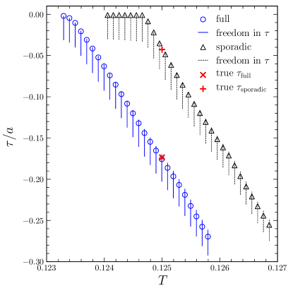
Figure 4 shows the minimum active fractions found for each , and the global minimum picking out the optimal . From our likelihood analysis we obtain the best fit parameters to be and for the full, and and for sporadic mock cases respectively (compared to the truth, , ). Any model lying above the curve is a valid fit to the data, but less efficient than the optima. We see that the global optimum is quite close to the truth. Note that this method gives a best fit, but not an uncertainty per se.
We can define an uncertainty by choosing to consider models with a bound on inefficiency such that the optimum behavior would not appear much less frequently than in 68.3% of simulated data sets. For example, a model with a larger than needed active window, hence , would be consistent with the data, but only rarely would its realizations be as restricted as the data, i.e. falling in narrower windows. “Efficient” models lie in the region above the minimization curve but below the dotted, nearly diagonal inefficiency curve (see Appendix A for its expression). Projecting to the axis defines the range in the period. For the full case this gives a range of , or uncertainty on the period. For the sporadic case the range is , or uncertainty (the tighter precision relative to the full case is due to the higher density, though fewer, windows; recall they both have the same total number of events, just distributed differently).

Figure 5 shows the phase parameter . It is tightly constrained when is at the minimum, but has a modest range when , for a given . Finally, we note that we crosschecked against two other optimization approaches, specifically simulated annealing by employing the dual_annealing routine from the SciPy optimization package and a MCMC sampler, and found the results are compatible (see Appendix B).
IV Application to SGR1935+2154
Real observational data can be more difficult, and scientifically rewarding. We apply our methods to actual measurements of the source SGR1935+2154, testing whether it exhibits PWB, and giving robust estimates of its period and active window fraction. These characteristics can constrain models of the origin of the emission and properties of the system.
SGR1935+2154, a magnetar within our Galaxy, was identified as the source of two FRBs occurring UT 2020 April 28 [9, 10]. The local nature makes measurements of the object and its environment much easier and with much greater detail. In fact, a linkage between the production of soft gamma bursts in this source and FRBs is naturally suggested: the same two events as the FRBs, with the appropriate delay due to dispersion by interstellar electrons, were detected by -ray instruments [23, 24, 25, 26, 27] (though some authors suggest that different source types may be responsible for these vs extragalactic FRBs [28]).
As an example of the constraining power of these measurements, in [8] the SGR1935+2154 soft gamma burst PWB period was found to be 231 days, but the binary comb model for FRB [29] is limited to periods days [30]. Such a model may perhaps be eliminated for SGR1935+2154 or other PWB long-period magnetars [8], pointing to other models such as isolated neutron star precession (e.g. [31]) as the source of periodicity, coupled with a nonperiodic emission mechanism. More generally, given an excellent knowledge of the PWB parameters, correlating additional observational properties with these parameters may shed further light on the physical mechanisms at play. For example, with robust knowledge of the phase of the window boundaries, one could look not only for correlations with the modulation period, but also for effects at the window boundaries in SGR burst intensity, fluence, and spectral characteristics. Comparison of the variation in soft gamma burst polarization measurements (coming from the next generation of instruments) with the PWB period and the window boundaries could shed light on the role of the magnetic field in these modulations, as well as in the role of magnetic field orientation in the emission mechanism.
Long term monitoring of SGR1935+2154 has provided several years of data from a number of -ray instruments. In [8], for some range of periods the data were folded at various trial periods, and the activity fraction – the fraction of a period that would be consistent with all event data, was calculated, and the period with the minimum activity fraction was taken to be the “best” period. That analysis did not provide an examination of the uncertainty in the period or active fraction. Its conclusion that there was actually a periodic windowed behavior arose from comparison to uniform random events. Here we use different methods and quantification, and a clustering analysis.
We apply our methods to burst data from the Third Interplanetary Network (IPN3 [32]). IPN3 includes numerous spacecraft with X-ray and gamma-ray sensitive instruments, but notably the Konus instrument on the Wind spacecraft. This instrument is in orbit around the sun at Lagrange point 1, far from earth, and so provides a nearly continuous, unobstructed view of the entire sky, and a more constant background than for low-earth orbit instruments. These are ideal properties for time series monitoring444While there is some heterogeneity in instruments and coverage, the main instruments other than Konus are in low earth orbit, without any long-term changing viewing zones and hence no bias for or against periods in the hundreds of days range. An analysis for particular sets of instruments was carried out in [8] and found results consistent with each other and the results here. .
Carrying out our procedure for identifying and characterizing PWB, we first examine the CDF, as in Fig. 1, but here applied to SGR1935+2154 data (159 events identified in the IPN3 SGR list for SGR1935+2154 as of 2021 February 1 [32]). Figure 6 shows the resulting CDF. While there are clearly episodes of activity and gaps of inactivity, it is difficult to tell by eye if there is PWB.

Applying the FOF method, we carry out the period analysis in Figure 7. While the activity window lengths and gaps scatter greatly, the pseudoperiods (sum of consecutive active window lengths and gap lengths) show an interesting pattern. We exhibit , and see a concentration around , or .

The FOF method gives the estimate for the period (not pseudoperiod ratio) of . While a broad estimation, due to some empty activity windows increasing the uncertainty, it still provides a useful prior for the more incisive likelihood analysis. In addition we find the activity window length and six active windows.
We proceed with our likelihood analysis and parameter determination of the SGR1935+2154 data in the same manner as the simulated cases of Sec. III. The final results determine a global optimal period and active fraction (i.e. ). Converting back to days by rescaling to the duration of observations, this implies the PWB has period days, with an active fraction of 55.4%. Figure 8 shows the results, along with the local optima boundary. Using the efficiency criterion, analysis of the SGR1935+2154 data yields a range of , or uncertainty on the period.

Figure 9 presents the estimation of the phase parameter, with a best estimate of , i.e. the first detected burst of the time series occurred 10% of the way through the activity window. The estimation of this is very tight () at , broadening as shown in the figure as one moves away from the local optima (here we show a shift by 0.02 from the minimum , the same fractional difference as the 0.01 shift used in Fig. 5).

Finally, we note that the FOF estimations for the period and active window length do include the likelihood optimization results of , (i.e. , and the optimization results lie well inside the prior information from the FOF analysis. Our results agree as well with those from [8].
V Conclusions
Astrophysical bursts occur in observations throughout the electromagnetic spectrum, from the radio to optical to gamma ray. Repeated outbursts indicate the source is not totally disrupted, and periodic bursting points at some physics connected with, e.g., rotation or an orbital companion. An intriguing middle ground that is becoming more recognized with further data is periodic windowed behavior, where activity windows, rather than the burst events themselves, have periodicity. This can also provide important clues to the astrophysical mechanism of the burst, and system characteristics.
Analysis methods for strict periodicity often fall short when dealing with PWB, as the duty cycle is important, activity windows can be empty of events, and the time series of events can be distributed in a complicated manner. We have emphasized that the lack of bursts carries critical information that must fold into the analysis, and we develop a time domain method that takes this into account.
The cumulative distribution function of event intervals works well at identifying whether or not PWB is a reasonable possibility. We test this technique for four distributions: uniform random, Weibull, PWB, and a special distribution with correlated clustering. Given reasonable indications identifying PWB from the CDF analysis, we then draw on the friends of friends technique from galaxy clustering to characterize the PWB. This FOF analysis delivers quantitative estimates of the period , active window length (and hence duty cycle ), and observing phase . For our test cases of mock data, the estimates accurately reconstruct the input and have precision for data with at least 100 events and populated windows. However, we view the FOF analysis as a guide toward carrying out a full likelihood analysis (where the FOF can serve in setting reasonable priors).
For the likelihood analysis we use an optimization grid approach, due to the low dimensionality of the parameter space, increased accuracy, and that the posterior surface is actually a broad plateau, not an isolated peak. However we do find consistent results with both a simulated annealing approach and a Markov Chain Monte Carlo approach. We minimize the duty cycle that agrees with the data, and find accurate estimates of the period to uncertainty on the mock data. Analyzing real observational data on the source SGR1935+2154 we first identify that PWB is reasonable for the data, and then characterize it as having period days, with uncertainty, and duty cycle .
Finding PWB for what is truly a random distribution is highly unlikely: if we consider the probability that a uniform distribution realization would avoid all the 10 spans of time that PWB predicts no activity (let alone have the active windows in a periodic pattern), this is . For a truly uniformly random distribution one could take into account not just the number of windows but the total number of events, so the probability would be . Nevertheless, the ultimate proof will be predictivity: if the values for the period and active fraction derived above are correct, the next two active windows (which admittedly are not guaranteed to have activity) are from June 1 - October 7, 2021 and January 18 - May 26, 2022 and we predict no activity outside of our active windows555On June 24, 2021 a burst was detected by the Fermi Gamma-Ray Space Telescope, in our predicted window. Equally importantly, no bursts were detected outside our predicted windows..
Numerous next generation time domain surveys in a wide range of wavelength bands (e.g. LSST [33] in the optical, DSA-2000 [34] and CMB-S4 [35] in the radio and submillimeter, wide-field instruments such as STROBE-X WFM [36] and SVOM ECLAIRs [37] in the X-ray/gamma ray bands) will greatly increase the database and diversity of repeating sources with possible PWB. The efficient methods presented here give a straightforward path for analysis, identification as PWB (vs, e.g., simply clustering), and its characterization. Accurate estimations of PWB, and the period, duty cycle, and phase, offer the potential for significant advances in understanding the physics of energetic bursts and the properties of the repeating outburst systems, in a wide variety of astrophysical contexts.
Acknowledgements.
We thank Alex Kim for helpful discussions. This work is supported in part by the Energetic Cosmos Laboratory. EL is supported in part by the U.S. Department of Energy, Office of Science, Office of High Energy Physics, under contract no. DE-AC02-05CH11231. This paper has made use of data of the Interplanetary Network (http://ssl.berkeley.edu/ipn3), maintained by K. Hurley.Appendix A Estimating Inefficiency
Many models, i.e. combinations of periods and active fractions , can fit the data. Trivially, a model that is always active, , will fit the burst data but be inefficient at doing so. That is, it allows bursts at any time but they seem to appear only within periodic windows. Such a formal fit is not informative. We therefore seek the most efficient fit as the most informative: the model with and its associated . However, models close to this are only a little inefficient, that is many realizations of such models would generate data still falling within the optimal window structure. Conversely, for models further away, such as all-active models, Monte Carlo simulations of such a model would show many instances that, while including the data, would also have predicted many bursts where none were seen. Hence it is inefficient (or, if you like, complete but not pure).
We seek a measure of the inefficiency, so that the region of efficient models can translate to a range, or uncertainty, of the period and active fraction. Consider a single window. If it is a little wider than optimal, then that model will fit the more restrictive data, but be somewhat inefficient at doing so. Suppose we want 68.3% of simulations of a model to not only match the data but also not give bursts outside the optimal windows. For one window, and one burst within the window, this means that models with are likely to be inefficient. For independent windows the inefficiencies multiply, so to obtain an efficiency each window can only contribute a factor . If we consider more than one burst within a window, we have to understand the coherence between bursts before we can quantitatively evaluate this, but gives an upper limit to the inefficiency so we stay with this.
Similarly, if the period is taken to be longer than optimal, this can also be inefficient. For a constant , a longer means a longer active window width . Again this adds inefficiency to each window, giving a factor for each window. There are further effects from the shift of the far and near sides of the windows, and the phase, but these contribute less when , . Under those conditions we simply multiply the two inefficiency factors to get to first order
| (5) |
We use this to define the diagonal inefficiency curves in Figs. 4 and 8. We have checked this gives a reasonable approximation under the conditions stated by running a suite of 1000 Monte Carlo realizations.
Appendix B Comparison to Direct Optimization
As mentioned in Sec. III, we have crosschecked our direct grid search optimization routine with a standard MCMC and a simulated annealing optimization. The direct grid search is innately more exact, and sufficiently efficient due to low dimensionality of our parameter space that we use it throughout the paper. We exhibit some results of the other two methods here.
Fig. 10 shows the MCMC samples generated using the Stan software [38] to find the global optimum model and explore the distribution of other combinations of parameters consistent with SGR1935+2154 data. It agrees well with our direct optimization. We also used the dual simulated annealing optimization routine dual_annealing [39] as a complementary approach to the grid search optimization to quickly find the best estimates of the global minimum. We randomly chose 25 initial points and found the dual annealing provided good estimates of the global minimum as well, as seen in Fig. 11.


References
- [1] R.B. Blackman, J.W. Tukey, Measurement of power spectra from the point of view of communication engineering (Dover, 1958)
- [2] D.H. Staelin, Proc. IEEE 57, 724 (1969)
- [3] J.T. VanderPlas, Understanding the Lomb-Scargle Periodogram, ApJS 236, 16 (2018) [arXiv:1703.09824]
- [4] K.M. Rajwade et al., Possible periodic activity in the repeating FRB 121102, MNRAS 495, 3551 (2020) [arXiv:2003.03596]
- [5] M. Cruces, L.G. Spitler, P. Scholz, R. Lynch, A. Seymour, J.W.T. Hessels, C. Gouiffès, G.H. Hilmarsson, M. Kramer, S. Munjal, Repeating behaviour of FRB 121102: periodicity, waiting times, and energy distribution, MNRAS 500, 448 (2021) [arXiv:2008.03461]
- [6] N. Oppermann, H-R. Yu, U-L. Pen, On the non-Poissonian repetition pattern of FRB121102, MNRAS, 475, 5109 (2018) [arXiv:1705.04881]
- [7] CHIME/FRB Collaboration, Periodic activity from a fast radio burst source, Nature 582, 351 (2020) [arXiv:2001.10275]
- [8] B. Grossan, Periodic Windowed Behavior in SGR1935+2154 SGR Bursts, arXiv:2006.16480
- [9] F. Kirsten, M.P. Snelders, M. Jenkins, K. Nimmo, J. van den Eijnden, J. Hessels, M. Gawronski, J. Yang, Detection of two bright radio bursts from magnetar SGR 1935 + 2154, Nature Astronomy 232 (2020) [arXiv:2007.05101]
- [10] C.D. Bochenek, V. Ravi, K.V. Belov, G. Hallinan, J. Kocz, S.R. Kulkarni, D.L. McKenna, A fast radio burst associated with a Galactic magnetar, Nature 587, 59 (2020) [arXiv:2005.10828]
- [11] G.Q. Zhang, Z-L. Tu, F.Y. Wang, Possible periodic activity in the short bursts of SGR 1806-20: connection to fast radio bursts, arXiv:2101.07923
- [12] E. Platts, A. Weltman, A. Walters, S.P. Tendulkar, J.E.B. Gordin, S. Kandhai, A living theory catalogue for fast radio bursts, Phys. Rep. 821, 1 (2019) [arxiv:1810.05836]
- [13] N.R. Lomb, Least-Squares Frequency Analysis of Unequally Spaced Data, Astroph. Space Sci. 39, 447 (1976)
- [14] J.D. Scargle, Studies in astronomical time series analysis. II. Statistical aspects of spectral analysis of unevenly spaced data, ApJ 263, 835 (1982)
- [15] J.I. Katz, Testing models of periodically modulated FRB activity, MNRAS 502, 4664 (2021) [arXiv:2012.15354]
- [16] A.C. Doyle, Silver Blaze, in The Memoirs of Sherlock Holmes (1892)
- [17] R.M. Soneira , P.J.E. Peebles, A computer model universe: simulation of the nature of the galaxy distribution in the Lick catalog, Astron. J. 83, 845 (1978)
- [18] P.J.E. Peebles, Large-scale Structure of the Universe, Princeton U. Press (1980)
- [19] S. Kullback, R. A. Leibler, On information and sufficiency, Ann. Math. Statistics, 22, 79 (1951)
- [20] F. Pérez-Cruz, Kullback-Leibler divergence estimation of continuous distributions, 2008 IEEE Int. Symp. on Information Theory, p. 1666, doi: 10.1109/ISIT.2008.4595271
- [21] J.P. Huchra, M.J. Geller, Groups of Galaxies. I. Nearby groups, ApJ 257, 423 (1982)
- [22] M. Davis, G. Efstathiou, C.S. Frenk, S.D.M. White, The Evolution of Large-Scale Structure in a Universe Dominated by Cold Dark Matter, ApJ 292, 371 (1985)
- [23] S.N. Zhang et al., Insight-HXMT X-ray and hard X-ray detection of the double peaks of the Fast Radio Burst from SGR 1935+2154, GCN 27675 (2020)
- [24] C.K. Li et al., HXMT identification of a non-thermal X-ray burst from SGR J1935+2154 and with FRB 200428, Nature Astronomy 36 (2021) [arXiv:2005.11071]
- [25] S. Mereghetti et al., INTEGRAL Discovery of a Burst with Associated Radio Emission from the Magnetar SGR 1935+2154, ApJL 898, L29 (2020) [arXiv:2005.06335]
- [26] M. Tavani, C. Casentini, A. Ursi, F. Verrecchia, A. Addis, An X-ray burst from a magnetar enlightening the mechanism of fast radio bursts, Nature Astronomy 31 (2021) [arXiv:2005.12164]
- [27] A. Ridnaia, S. Golenetskii, R. Aptekar, D. Frederiks, M. Ulanov, D. Svinkin, A. Tsvetkova, A. Lysenko, T. Cline, Konus-Wind observation of hard X-ray counterpart of the radio burst from SGR 1935+2154, GCN 27669 (2020)
- [28] B. Margalit, P. Beniamini, N. Sridhar, B.D. Metzger, Implications of a Fast Radio Burst from a Galactic Magnetar, ApJL 899, L27 (2020) [arXiv:2005.05283]
- [29] K. Ioka, B. Zhang, A Binary Comb Model for Periodic Fast Radio Bursts, ApJL 893, L26 (2020) [arXiv:2002.08297]
- [30] X. Zhang, H. Gao, What binary systems are the most likely sources for periodically repeating FRBs?, MNRAS 498, L1 (2020) [arXiv:2006.10328]
- [31] T. Akgün, B. Link, I. Wasserman, Precession of the Isolated Neutron Star PSR B1828-11, MNRAS 365, 653 (2006) [arXiv:astro-ph/0506606]
- [32] K. Hurley, Retrieved from The Third Interplanetary Network (2021 February 1), http://www.ssl.berkeley.edu/ipn3
- [33] LSST Dark Energy Science Collaboration, The LSST Dark Energy Science Collaboration (DESC) Science Requirements Document, arXiv:1809.01669
- [34] G. Hallinan et al., DSA-2000 – A Radio Survey Camera, arXiv:1907.07648
- [35] K. Abazajian et al., CMB-S4 Science Case, Reference Design, and Project Plan, arXiv:1907.04473
- [36] P.S. Ray et al., STROBE-X: X-ray Timing and Spectroscopy on Dynamical Timescales from Microseconds to Years, arXiv:1903.03035
- [37] O. Godet et al., The X-/gamma-ray camera ECLAIRs for the gamma-ray burst mission SVOM, Proc. SPIE Space Telescopes and Instrumentation 2014: Ultraviolet to Gamma Ray, 9144: 914424 (2014) [arXiv:1406.7759]
- [38] Stan Development Team (2021). “PyStan: the Python interface to Stan.” Python package version 3.1.1, http://mc-stan.org/
- [39] P. Virtanen et al., SciPy 1.0–Fundamental Algorithms for Scientific Computing in Python, Nature Methods 17, 261 (2020) [arXiv:1907.10121]