Distance and the Goeritz groups of bridge decompositions

It is well known that any closed orientable $3$-manifold $M$ is obtained by gluing two handlebodies $V^{+}$ and $V^{-}$ of the same genus along their boundaries. Such a decomposition of $M$ is called a Heegaard splitting, and the common boundary $\Sigma$ of $V^{+}$ and $V^{-}$ is called the Heegaarrd surface of the splitting. The distance of a Heegaard splitting $M=V^{+}\cup_{\Sigma}V^{-}$ is a measure of complexity introduced by Hempel [5]. It is defined to be the distance between the sets of meridian disks of $V^{+}$ and $V^{-}$ in the curve graph of $\Sigma$. The distance has successfully provided a way of describing the topology and geometry of $3$-manifolds.

A bridge decomposition of a link $L$ in a closed orientable $3$-manifold $M$ is a Heegaard splitting $M=V^{+}\cup_{\Sigma}V^{-}$ such that $L$ intersects each of $V^{+}$ and $V^{-}$ in properly embedded trivial arcs. When the genus of the surface $\Sigma$, called a bridge surface, is $g$, and the number of components of $V^{\pm}\cap L$ is $n$, we particularly call such a decomposition a $(g,n)$-decomposition of $L$. The distance is also defined for a bridge decomposition in the same way as in the case of a Heegaard splitting, and many results about Heegaard splittings have been extended to bridge decompositions. For example, Bachman-Schleimer [1] showed that the distance of a bridge decomposition of a knot is bounded above by the Euler characteristic of an essential surface in the complement of the knot, which is a generalization of a result of Hartshorn [4]. The arguments in [1] apply to the case of links as well, and their results, in particular, imply that if the distance of a link in a $3$-manifold is at least $5$, then the complement of the link admits a complete hyperbolic structure of finite volume. (The definition of the distance in this paper is slightly different from that in [1], see Section 1.3.) As another example, Tomova [17] gave a sufficient condition for uniqueness of bridge decompositions of knots in terms of the distances and the Euler characteristics of bridge surfaces, which is a generalization of a result of Sharlemann-Tomova [16].

In this paper, we are interested in the Goeritz group of a bridge decomposition. The Goeritz group (or the mapping class group) of a Heegaard splitting is defined to be the group of isotopy classes of self-diffeomorphisms of the ambient $3$-manifold that preserve the splitting setwize. Namazi [14] showed that for each topological type of Heegaard surface there exists a constant $C$ such that if the distance is at least $C$, then the Goeritz group is a finite group. Johnson [9] had refined this result by showing the constant $C$ can be taken to be at most $4$ independently of the genus of the Heegaard surface. The concept of Goeritz group has also been extended for bridge decompositions in [6]. In that paper, a variation of Namazi and Johnson’s result for the case of bridge decomposition was obtained: it was shown that the constant $C$ for the finiteness of the Goeritz group can be taken uniformly to be at most $3796$. The main result of the paper is the following, which improves the above mentioned result of [6].

Theorems 0.1 is proved by extending the argument of [9] to the case of bridge decompositions. In fact, the major part of the proof is devoted to show the following.

The paper is organized as follows. In Section 1, we review basic definitions and properties of the distance and the Goeritz group of a bridge decomposition. In Section 2, we review the theory of sweep-outs, which is the main tool of the paper. In Section 3, we give the proof of Theorem 3.1. Finally, in Section 4, we give the proof of Theorem 0.1.

We work in the smooth category. Throughout the paper, we will use the following notations and conventions:

• •

  Given two sets $A$ and $B$, we denote by $A-B$ or $A_{B}$ the relative complement of $B$ in $A$.

• •

  For a topological space $X$, we denote by $|X|$ the number of connected components of $X$. For a subset $Y\subset X$, we denote by $\mathrm{Cl}(Y;X)$ or $\mathrm{Cl}(Y)$ the closure of $Y$ in $X$.

• •

  For simplicity, we will not distinguish notationally between simple closed curves in a surface and their isotopy classes throughout.

We review the basic theory of sweep-outs. The main references of this section are Kobayashi-Saeki [12] and Johnson [10]. In the following, let $M$ be a closed orientable $3$-manifold, $L$ a link in $M$, and $(M,L;\Sigma)$ a $(\mathrm{genus}(\Sigma),n)$-decomposition of $L$ throughout.

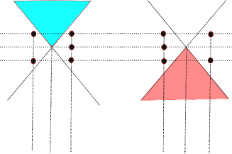
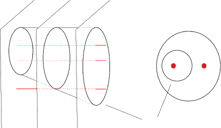
We note that any bridge decomposition admits a sweep-out. For simplicity, we shall always assume further that the spines $f^{-1}(\pm 1)$ are uni-trivalent graphs, and the intersection of the spines and $L$ is exactly the set of vertices whose valency is one. See Figure 1.

A smooth map $F$ from a $3$-manifold $N$ into $\mathbb{R}^{2}$ is said to be stable if there exists a neighborhood $U(F)$ of $F$ in the space of smooth maps $C^{\infty}(N,\mathbb{R}^{2})$ with the following property: for any $G\in U(F)$, there exist diffeomorphisms $\varphi:N\rightarrow N$ and $\psi:\mathbb{R}^{2}\rightarrow\mathbb{R}^{2}$ satisfying $G\circ\varphi=\psi\circ F$. The image of the set of singular points of the stable map is called the discriminant set.

Let $f$ and $g$ be sweep-outs of $(M,L)$. Due to Kobayashi-Saeki [12], the map $f\times g:M\rightarrow[-1,1]\times[-1,1]$ can be perturbed so that $f\times g$ is stable in the complement of spines of $f$ and $g$. In the following, whenever we consider the product of sweep-outs, we slightly perturb it to be stable. Let $\Gamma$ be the closure in $[-1,1]\times[-1,1]$ of the union of the discriminant set of $f\times g$ and the image of $L$ under the map $f\times g$. Then $\Gamma$ is naturally equipped with a structure of a finite graph of valency at most four. Such a finite graph is called the (Rubinstein-Scharlemann) graphic defined by $f\times g$.

Each point $(s,t)$ in the interior of the square $[-1,1]\times[-1,1]$ corresponds to the intersection of two level surfaces $\Sigma_{s}:=f^{-1}(s)$ and $\Sigma^{\prime}_{t}:=g^{-1}(t)$. We note that the surfaces $\Sigma_{s}$ and $\Sigma^{\prime}_{t}$ always intersect $L$ transversely by definition. If the point $(s,t)$ lies in the complementary region of the graphic $\Gamma$, then the surfaces $\Sigma_{s}$ and $\Sigma^{\prime}_{t}$ intersect transversely and $\Sigma_{s}\cap\Sigma_{t}\cap L=\emptyset$. If $(s,t)$ lies in the interior of an edge of $\Gamma$, then either

• •

  $\Sigma_{s}$ and $\Sigma^{\prime}_{t}$ share a single tangent point, and that point is a non-degenerate critical point of both $f|_{\Sigma^{\prime}_{t}}$ and $g|_{\Sigma_{s}}$, see Figure 2 (i) and (ii); or

• •

  $\Sigma_{s}$ and $\Sigma^{\prime}_{t}$ intersect transversely, and $\Sigma_{s}\cap\Sigma^{\prime}_{t}\cap L$ is a single point, see Figure 2 (iii).

If $(s,t)$ is at a $4$-valent vertex of $\Gamma$, then either

• •

  $\Sigma_{s}$ and $\Sigma^{\prime}_{t}$ share exactly two tangent points, and those points are non-degenerate critical points of both $f|_{\Sigma^{\prime}_{t}}$ and $g|_{\Sigma_{s}}$;

• •

  $\Sigma_{s}$ and $\Sigma^{\prime}_{t}$ share a single tangent point, and that point is a non-degenerate critical point of both $f|_{\Sigma^{\prime}_{t}}$ and $g|_{\Sigma_{s}}$. Further, $L$ intersects $\Sigma_{s}\cap\Sigma^{\prime}_{t}$ at a point where $\Sigma_{s}$ and $\Sigma^{\prime}_{t}$ intersect transversely; or

• •

  $\Sigma_{s}$ and $\Sigma^{\prime}_{t}$ intersect transversely, and $\Sigma_{s}\cap\Sigma^{\prime}_{t}\cap L$ consists of exactly two points.

If $(s,t)$ is at a $2$-valent vertex of $\Gamma$, then $\Sigma_{s}$ and $\Sigma^{\prime}_{t}$ share a single tangent point, and that point is a degenerate critical point of both $f|_{\Sigma^{\prime}_{t}}$ and $g|_{\Sigma_{s}}$. See Figure 3.

Each $1$- or $3$-valent vertex is in the boundary of the square, and it corresponds to the point where the level surface of one of the two sweep-outs is tangent to the spine of the other sweep-out.

The following is Lemma $34$ of Johnson [10].

Let $f$ and $g$ be sweep-outs associated to $(M,L;\Sigma)$. Let $t,s\in(-1,1)$. Set $\Sigma_{s}:=f^{-1}(s)$, $\Sigma_{t}^{\prime}:=g^{-1}(t)$, ${V_{s}}^{-}:=f^{-1}([-1,s])$, ${V_{s}}^{+}:=f^{-1}([s,1])$, ${V^{\prime}_{t}}^{-}:=g^{-1}([-1,t])$ and ${V^{\prime}_{t}}^{+}:=g^{-1}([t,1])$.

Let $\mathscr{R}_{a}$ ($\mathscr{R}_{b}$, respectively) denote the set of all points $(s,t)\in[-1,1]\times[-1,1]$ such that $\Sigma_{s}$ is mostly above (mostly below, respectively) $\Sigma_{t}^{\prime}$. The regions $\mathscr{R}_{a}$ and $\mathscr{R}_{b}$ are bounded by the edges of the graphic. Note that a point $(s,t)$ near $[-1,1]\times\{-1\}$ is labeled by $\mathscr{R}_{a}$ because ${V^{\prime}_{t}}^{-}$ lies within a small neighborhood the spine of $g$, and the all intersections of ${V^{\prime}_{t}}^{-}$ and $\Sigma_{s}$ must consist of disks. Similarly, a point $(s,t)$ near $[-1,1]\times\{1\}$ is labeled by $\mathscr{R}_{b}$. Also, by definition, both regions $\mathrm{Cl}(\mathscr{R}_{a})$ and $\mathrm{Cl}(\mathscr{R}_{b})$ are vertically convex, that is, if a point $(s,t)$ is in $\mathrm{Cl}(\mathscr{R}_{a})$ ($\mathrm{Cl}(\mathscr{R}_{b})$, respectively), then so is $(s,t^{\prime})$ for any $t^{\prime}\leq t$ ($t^{\prime}\geq t$, respectively).

In what follows, we assume that $(\mathrm{genus}(\Sigma),n)\not=(0,1),(0,2),(1,1)$. We say that $g$ spans $f$ if there there exists $t\in[-1,1]$ such that the horizontal arc $[-1,1]\times\{t\}$ intersects both $\mathscr{R}_{a}$ and $\mathscr{R}_{b}$. Otherwise, we say that $g$ splits $f$. See Figure 6.

We say that $g$ spans $f$ positively if there exist points $(a,t)\in\mathscr{R}_{a}$ and $(b,t)\in\mathscr{R}_{b}$ with $b<a$.

Let $(M,L)=(V^{+},V^{+}\cap L)\cup_{\Sigma}(V^{-},V^{-}\cap L)$ be a $(\mathrm{genus}(\Sigma),n)$-decomposition of a link $L$ in a closed orientable $3$-manifold $M$, and suppose that $(\mathrm{genus}(\Sigma),n)\not=(0,1),(0,2),(1,1)$. Recall that $d_{\mathcal{PD}}(M,L;\Sigma)=d_{\mathrm{C}(\Sigma_{L})}(\mathcal{PD}(V^{+}_{L}),\mathcal{PD}(V^{-}_{L}))$. The goal of this section is to show the following.

We prove Theorem 3.1. We first note that, by Lemma 1.2, we may assume the following.

Let $f:M\rightarrow[-1,1]$ be a sweep-out of $(M,L)$ with $f^{-1}(0)=\Sigma$, and $g$ the result of perturbing $f$ slightly. Let $[\phi]$ be in the kernel of $\eta$. Then, there exists an ambient isotopy $\{\Phi_{r}:M\rightarrow M\}_{r\in[0,1]}$ such that $\Phi_{0}=\mathrm{id}_{M}$, $\Phi_{1}=\phi$, and $\Phi_{r}(L)=L$ for all $r\in[0,1]$. We can assume that $\{\Phi_{r}\}_{r\in[0,1]}$ satisfies the conditions described in Lemma 2.1, that is, only a finitely many element in the $1$-parameter family $\{g_{r}:=g\circ\Phi_{r}\}_{r\in[0,1]}$ of sweep-outs of $(M,L)$ is non-generic.

References

- [1] D. Bachman and S. Schleimer, Distance and bridge position. Pacific J. Math. 219 (2005), no. 2, 221–235.
- [2] R. Blair, M. Campisi, J. Johnson, S. A. Taylor and M. Tomova, Exceptional and cosmetic surgeries on knots, Math. Ann. 367 (2017), no. 1-2, 581–622.
- [3] W. Haken, Some results on surfaces in -manifolds, Studies in Modern Topology pp. 39–98 Math. Assoc. Amer. (distributed by Prentice-Hall, Englewood Cliffs, N.J.) 1968.
- [4] K. Hartshorn, Heegaard splittings of Haken manifolds have bounded distance. Pacific J. Math. 204 (2002), no. 1, 61–75.
- [5] J. Hempel, -manifolds as viewed from the curve complex, Topology 40 (2001), no. 3, 631–657.
- [6] S. Hirose, D. Iguchi, E. Kin and Y. Koda, Goeritz groups of bridge decompositions, to appear in Int. Math. Res. Not.
- [7] K. Ichihara and J. Ma, A random link via bridge position is hyperbolic, Topology Appl. 230 (2017), 131–138.
- [8] Y. Jang, Distance of bridge surfaces for links with essential meridional spheres. Pacific J. Math. 267 (2014), no. 1, 121–130.
- [9] J. Johnson, Mapping class groups of medium distance Heegaard splittings, Proc. Amer. Math. Soc. 138 (2010), no. 12, 4529–4535.
- [10] J. Johnson, Bounding the stable genera of Heegaard splittings from below. J. Topol. 3 (2010), no. 3, 668–690.
- [11] J. Johnson, Automorphisms of the three-torus preserving a genus-three Heegaard splitting. Pacific J. Math. 253 (2011), no. 1, 75–94.
- [12] T. Kobayashi and O. Saeki, The Rubinstein-Scharlemann graphic of a 3-manifold as the discriminant set of a stable map. Pacific J. Math. 195 (2000), no. 1, 101–156.
- [13] M. Korkmaz and A. Papadopoulos, On the arc and curve complex of a surface. Math. Proc. Cambridge Philos. Soc. 148 (2010), no. 3, 473–483.
- [14] H. Namazi, Big Heegaard distance implies finite mapping class group, Topology Appl. 154 (2007), 2939–2949.
- [15] H. Rubinstein and M. Scharlemann, Comparing Heegaard splittings of non-Haken -manifolds, Topology 35 (1996), 1005–1026.
- [16] M. Scharlemann and M. Tomova, Alternate Heegaard genus bounds distance. Geom. Topol. 10 (2006), 593–617.
- [17] M. Tomova, Multiple bridge surfaces restrict knot distance. Algebr. Geom. Topol. 7 (2007), 957–1006.