Disorder-induced delocalization in flat-band systems with quantum geometry
Abstract
We investigate the transport properties of flat-band systems by analyzing a one-dimensional metal/flat-band/metal junction constructed on a Lieb lattice with an infinite band gap. Our study reveals that disorders can induce delocalization and enable the control of transmission through quantum geometry. In the weak disorder regime, transmission is primarily mediated by interface-bound states, whose localization length is determined by the quantum geometry of the system. As disorder strength increases, a zero-energy transmission channel—absent in the clean system—emerges, reaches a maximum, and then diminishes inversely with disorder strength in the strong disorder limit. In the strong disorder regime, the transmission increases with the localization length and eventually saturates when the localization length becomes comparable to the link size. Using the Born approximation, we attribute this bulk transmission to a finite velocity induced by disorder scattering. Furthermore, by analyzing the Bethe-Salpeter equation for diffusion, we propose that the quantum metric provides a characteristic length scale for diffusion in these systems. Our findings uncover a disorder-driven delocalization mechanism in flat-band systems that is fundamentally governed by quantum geometry. This work provides new insights into localization phenomena and highlights potential applications in designing quantum devices.
Introduction.— The Berry curvature and quantum metric are fundamental geometric quantities that characterize the electronic structure of crystalline solids. These quantities form the quantum geometric tensor [1] , where and represent the real and imaginary parts, respectively. This tensor provides a complete description of the local geometry of Bloch states in momentum space. The Berry curvature , analogous to a magnetic field in momentum space, has been extensively studied, particularly in the context of topological insulators and superconductors [2, 3] over the past decades. The quantum metric , on the other hand, measures the distance between the Bloch states [4, 5] in momentum space. Recently, there has been growing interest in understanding the role of the quantum metric in various physical phenomena, such as the nonlinear anomalous Hall effect [6, 7], fractional quantum Hall [8, 9], fractional Chern insulators [10, 11], and optical responses [12, 13, 14].
In recent years, flat-band systems have gained significant attention due to the quenched kinetic energy. These systems are characterized by energy bands that remain constant regardless of the crystal momentum. The interplay between flat bands and quantum geometry has revealed intriguing physics, particularly in the context of moiré materials [15, 16]. These materials provide an intrinsic platform with isolated narrow or flat bands, giving rise to a rich array of phenomena such as correlated insulating phases [17, 18], superconductivity [19, 20], anti-/ferromagnetism [21, 22], and exciton [23, 24]. Importantly, it has been emphasized that the quantum metric plays a crucial role in shaping the physical properties of flat-band systems [25, 26], as traditional understanding may fail due to the vanishing Fermi velocity () or the divergent effective mass.
One of the primary challenges in studying flat-band systems arises from the lack of characteristic length scales or energy scales typically derived from the Fermi velocity or effective mass. For instance, the conventional coherence length formula , where represents transition temperature, may no longer accurately describe the behavior of flat-band superconductors. Recent progress in this field has suggested that a quantum metric length can emerge as the relevant scale determining the coherence length in a flat-band superconductor [27, 28]. Furthermore, the quantum metric length has been shown to govern the size of Majorana fermions [29], introducing a new, controllable degree of freedom.
Alongside these developments, traditional models for electrical conductivity [30], which rely heavily on band dispersion and electron mobility, face significant challenges when applied to flat-band systems. The absence of band dispersion in these materials creates a unique scenario where conventional understanding about charge transport breaks down since any relevant perturbations such as interaction [31, 32, 33, 34] and disorder effect [35, 36, 37, 38] can lift the macroscopic degeneracy. This raises intriguing questions about the contribution of the quantum metric towards quantum transport properties, with flat-band systems serving as intrinsic platforms for study, due to the absence of band dispersion. Additionally, the influence of disorder on transport in these systems remains an open and important area of investigation.
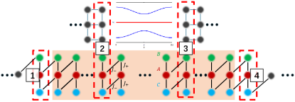
In light of these considerations, we aim to explore the effects of the disorder on the quantum transport properties of flat-band systems of quantum geometry. Specifically, we construct a metal/flat-band material/metal (M/FB/M) junction, where the flat-band system is realized by a Lieb lattice, and perform both two-terminal and four-terminal measurements [39] (see Fig. 1). In the absence of disorder (clean limit), transport is solely mediated by interface-bound states, whose localization length is tied to the quantum geometry effect of Bloch waves. Unlike the clean case, introducing disorder activates bulk-state transmission at zero energy, significantly enhancing transport compared to the clean limit.
M/FB/M junction.— The M/FB/M junction consists of a Lieb lattice as the link in the middle connecting the metallic leads. We first consider the two-terminal measurements with lead 1 and 4. The full Hamiltonian then can be split into several parts
| (1) |
The first part is the Lieb lattice [29] consists of three orbitals, labeled A, B, and C, with corresponding annihilation operators and . The Hamiltonian is given by
| (2) |
where and is the unit cell index. The Lieb lattice possesses one flat band and two dispersive bands, which are separated by a band gap . The Bloch state on the flat band possesses finite quantum metric,
| (3) |
In previous studies [27, 28, 29], it has been shown that the quantum metric can shape the properties of flat-band systems.
The second part is metallic leads described by simple tight-binding models with nearest-neighboring hopping
| (4) |
where being the fermion annihilation operator on the site with orbital index omitted. In the two-terminal measurement, Lead 1 and 4 are single-site chains connected to the floating site of the Lieb lattice while lead 2 and 3 are isolated to probe the bound states. In contrast, for the four-terminal measurement, we utilize three-site chains that are attached to the unit cell located at the central Lieb lattice to investigate bulk transport. For later convenience, we fix the chemical potential by setting .
The last part is the contact Hamiltonian which links the Lieb lattice with leads with coupling strength ,
| (5) |
Notice that although we choose the boundary condition for Lead 1 and 4 by fixing site coupling of the Lieb lattice, the other possible couplings will only change the results quantitatively. In this paper, we study the quantum transport of the M/FB/M junction with the setup in Fig. 1. In the clean limit, we perform the two-terminal measurement, while a four-terminal measurement is conducted in the presence of disorders. We first identify the exact wave functions of interface bound states which can facilitate transmittance. In the numerical calculations, unless otherwise specified, we set and while works as the unit of energy.
Bound state construction.— In the clean limit, two interface bound states can be created with a tunable localization length. We provide a methodology for calculating the exact wave function for bound states. We fix the energy of the bound states close to the flat band, and then the bound state wave function can be constructed with the sub-Hilbert space of . By exploring the flatband Bloch wave, we can find that A-sublattice sites do not contribute. Thus, we extend the condition to the bound states when . In this case, the Schrödinger equation for the Lieb lattice () is reduced to two simple recursive relations,:
| (6) | |||
| (7) |
We will focus on the interface bound states. For small , we have the general solutions to the recursive relations,
| (8) |
where and are the components of the wave function at the left-most site (). The B(C)-component interface state originates from the right(left) interface with the localization length . At , we have large degeneracy for bound states as long as vanishes. However, these bound states are unstable and can be smeared by the scattering waves. Thus, in the clean limit, we may not expect transmission from bulk states. For transmission to occur, the bound states need to have finite energy.
When specific to the finite energy , we can assume that the form of B, C-components in Eq. (8) is still valid, while takes on a perturbatively small value. The A-component can be obtained by an additional set of recursion relations along with Eqs. (6) and (7):
| (9) | ||||
| (10) |
By substituting in and with Eq. (8), we arrive at
| (11) |
The amplitude of is of the order , which is consistent with our assumption. The boundary condition, namely, the connection to the leads can determine and . Therefore, we reach the bound state solutions. With the effect of the external leads included, we can derive the transmission based on bound states.
Transmission without disorder.— Having solved the exact wavefunction within the Lieb lattice, we can now determine the transmission that originates from the interface-bound states. In the one-dimensional case, given an incoming wave with finite energy , we will have two bound states that center at two interfaces, respectively.
We start with an incoming incident wave from the left lead with energy , and corresponding wave vector . We assume reflected wave in the left lead, and transmitted wave in the right lead, where and satisfy the continuity condition . By solving the full wave functions, (details in SM), we can obtain the transmittance for as , where is the exponential decay factor of the bound state. Different from a conventional metal-insulator-metal junction with a dispersive band [40], has two maximum peaks at with . There is no phase difference between the incoming and transmitted waves at , indicating a destructive effect of reflected waves. Moreover, the transmission vanishes when approaches zero, namely, there is no transmission contribution from bound states. As we will see later, an enhancement of the transmission can occur when we involve disorder.
For the short junction limit, we have the perfect transmission with at . On the other hand, when the length of the junction is comparable to the localization length, the transmittance can be simplified to
| (12) |
which is maximal at with , and recovers the case of the weak transmission limit of a square trap. Eq. (12) resembles the effect of a transport system with two channels separated by energy . We can take as the characteristic energy scale for such an M/FB/M junction. In SM, we provide an alternate approach to derive the transmission within the M/FB/M junction using Green’s function method, which gives rise to the same transmission profile as in Eq. (12) under the long junction limit.
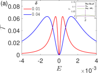
Numerical result in the clean limit.— We can demonstrate the theoretical predictions on the transmission profile via the two-terminal measurement. We can characterize the transmission profile by two key features: the maximal transmittance and the corresponding peak energy. In Fig. 2(a), the maximal transmittance matches the trend based on the wave function calculations. Specifically, in the case of the long junction , the maximal transmittance decays exponentially as the junction length increases, with a localization length . Furthermore, as shown in Fig. 2(b), the peak location is slightly smaller than the theoretical prediction . This discrepancy is due to the negligence of the higher-order terms in in the previous analytical calculation. In SM, we give the complicated exact form of the transmission, whose derivation is tedious. However, the prediction remains valid when the junction is long enough (), where the peak location approaches a constant value close to .
To clarify the role of the flat band in transport, we can compare the transmission profile of the Lieb lattice with the transmission profile of a two-band model without a flat band. The two-band model is constructed to contain the same dispersive bands as the Lieb lattice except for the removal of the flat band. When the flat band is removed, the transmission is strongly suppressed by an order of weaker, as shown in the inset of Fig. 2(a). Furthermore, the transmission profile reduces to the tunnel junction case with a single peak and a full width at half maximum (FWHM) on the order of . Thus, we can conclude that the significant overall transmission as well as its two-peak profile is enabled by the flat band, where the small energy scale emerges, allowing transmission to happen around the flat band.
Disorder-induced delocalization.— We will now explore the effects of disorder in the system. We introduce the Anderson’s onsite disorder, described by the Hamiltonian
| (13) |
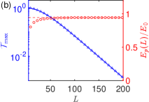
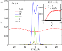
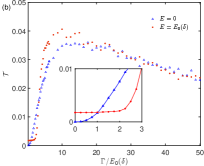
denotes the random onsite energy, uniformly distributed in the range . Based on the insights from interface bound states, we expect a series of bound states to emerge due to disorder, potentially triggering transport from bulk states. To minimize the impact of interface-bound states, we can use a four-terminal device and perform measurements between Leads 2 and 3, as illustrated in Fig. 1. The transmission profiles are shown in Figs. 3(a) and (b). Notably, the interface-bound state provides an energy scale . Fig. 3(a) displays the transmission behavior at various disorder strengths. We observe two peaks at when . As the disorder strength increases to , transport from bulk states gradually becomes dominant. In the strong disorder limit, , a plaquette structure emerges. A finite zero-energy transmission , which is absent in the clean limit (as shown in Fig. 2), characterizes the metallic properties of the flat band in the presence of disorder. Initially, increases as and peaks at (see Fig. 3). In the strong disorder limit, decays as , exhibiting typical conductivity behavior in a one-dimensional system. Such delocalization for a flat band is unexpected without considering quantum geometry. Inspired by the interface bound states, increasing the localization length enhances zero-energy transmission, which eventually saturates, as illustrated in the inset of Fig. 3.
To understand the dependence of the transmission on the junction length, We can use the localization length as the characteristic length scale for the diffusion transport, as one may anticipate the bound state can be excited by disorders. The disorder can lead to a broadening of the flat band. We can assume the disorder averaged for , otherwise . Here denotes the disorder average. For the case of weak disorder or the short junction where only one scattering process is effective during transmission, the transmission will become for . Thus, an enhancement is driven by the broadening of the transmission profiles of the interface bound states to zero energy. For the case of a stronger disorder or a long junction, multiple scattering processes occur as the localization length is greater than the effective distance of two impurities. By averaging the positions of the impurities, we can argue that where the factor is the effective density of states due to disorder. When , we have linear dependency and when , we reach constant value , which is consistent with Fig. 3(a). We have included calculations of a single pair of impurities within SM.
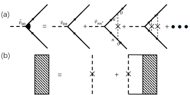
Diffusion transport.—We can discuss more about the transmission at the strong disorder limit of a long junction. Naively, a flat band without dispersion possesses a vanishing velocity. However, according to the Kubo-Greenwood formula, , we should have a finite velocity operator. We can make the crudest of approximations, . Then we apply the Born approximation diagrammatically as Fig. 4(a). The zeroth order vanishes and thus the leading order refers to the diagram involving single disorder scattering. The dominant contribution arises from the interband velocity which is proportional to the band gap with , respectively being the flat band and others. From the dimensional counting, we indeed find a finite velocity operator: for , which gives rise to . We do not have such correction from disorder for a band with trivial quantum geometry. Therefore, we can claim that the disorders mediate zero-energy transmission.
To explain the transmission’s size dependence, we try to calculate the diffusion length by considering the impurity vertex which satisfies the Bethe-Salpeter equation restricted on the flat band (see Fig. 4(b)). Formally, such a vertex involves the overlap . For small quantum metric, we have with , indicating that the quantum metric can provide a length scale as the diffusion length. It goes beyond the present scope for a comprehensive quantum theory, which we leave for future work.
Conclusion.— Flat-band materials such as moiré patterns [15], Kagome lattices [41], artificial quantum dot arrays [42] or optical lattice [43] could be used to construct M/FB/M junctions. The quantum geometry could be tuned by adjusting parameters like twist angle or lattice geometry, making these materials appealing for realizing the M/FB/M junction concept. Moreover, the M/FB/M junction concept can be generalized to a photonic crystal, which could function as an ideal frequency filter. These experiments would not only validate the theoretical predictions but also pave the way for novel quantum devices exploiting the unique transport properties of flat-band systems. Additionally, our numeric shows that disorder does not suppress transport in flat-band systems, but instead enhances it, also shedding light on why realistic flat-band systems, in particular van der Waals materials such as twisted bilayer graphene, where disorder should play a significant role intrinsically, still show robust signatures of transport at low charge carrier density.
Acknowledgements.
We thank Patrick A. Lee, Tai-Kai Ng, Roderich Moessner, and Haijing Zhang for their valuable discussions. K. T. L. acknowledges the support of the Ministry of Science and Technology, China, and the Hong Kong Research Grants Council through Grants No. 2020YFA0309600, No. RFS2021-6S03, No. C6025-19G, No. AoE/P-701/20, No. 16310520, No. 16310219, No. 16307622, and No. 16309223.References
- Provost and Vallee [1980] J. P. Provost and G. Vallee, Riemannian structure on manifolds of quantum states, Communications in Mathematical Physics 76, 289 (1980).
- Hasan and Kane [2010] M. Z. Hasan and C. L. Kane, Colloquium: Topological insulators, Reviews of Modern Physics 82, 3045 (2010), arXiv:1002.3895 [cond-mat.mes-hall] .
- Qi and Zhang [2011] X.-L. Qi and S.-C. Zhang, Topological insulators and superconductors, Reviews of Modern Physics 83, 1057 (2011), arXiv:1008.2026 [cond-mat.mes-hall] .
- Anandan and Aharonov [1990] J. Anandan and Y. Aharonov, Geometry of quantum evolution, Phys. Rev. Lett. 65, 1697 (1990).
- Resta [2011] R. Resta, The insulating state of matter: a geometrical theory, European Physical Journal B 79, 121 (2011), arXiv:1012.5776 [cond-mat.mtrl-sci] .
- Wang et al. [2023] N. Wang, D. Kaplan, Z. Zhang, T. Holder, N. Cao, A. Wang, X. Zhou, F. Zhou, Z. Jiang, C. Zhang, S. Ru, H. Cai, K. Watanabe, T. Taniguchi, B. Yan, and W. Gao, Quantum-metric-induced nonlinear transport in a topological antiferromagnet, Nature (London) 621, 487 (2023), arXiv:2306.09285 [cond-mat.mes-hall] .
- Kaplan et al. [2024] D. Kaplan, T. Holder, and B. Yan, Unification of Nonlinear Anomalous Hall Effect and Nonreciprocal Magnetoresistance in Metals by the Quantum Geometry, Phys. Rev. Lett. 132, 026301 (2024), arXiv:2211.17213 [cond-mat.mes-hall] .
- Haldane [2011] F. D. M. Haldane, Geometrical Description of the Fractional Quantum Hall Effect, Phys. Rev. Lett. 107, 116801 (2011), arXiv:1106.3375 [cond-mat.mes-hall] .
- Haldane [2023] F. D. M. Haldane, Incompressible Quantum Hall fluids as Electric Quadrupole fluids, arXiv e-prints , arXiv:2302.12472 (2023), arXiv:2302.12472 [cond-mat.str-el] .
- Abouelkomsan et al. [2023] A. Abouelkomsan, K. Yang, and E. J. Bergholtz, Quantum metric induced phases in Moiré materials, Physical Review Research 5, L012015 (2023), arXiv:2202.10467 [cond-mat.str-el] .
- Wu et al. [2024] A.-K. Wu, S. Sarkar, X. Wan, K. Sun, and S.-Z. Lin, Quantum metric induced quantum Hall conductance inversion and reentrant transition in fractional Chern insulators, arXiv e-prints , arXiv:2407.07894 (2024), arXiv:2407.07894 [cond-mat.str-el] .
- Ahn et al. [2022] J. Ahn, G.-Y. Guo, N. Nagaosa, and A. Vishwanath, Riemannian geometry of resonant optical responses, Nature Physics 18, 290 (2022), arXiv:2103.01241 [cond-mat.mes-hall] .
- Holder et al. [2020] T. Holder, D. Kaplan, and B. Yan, Consequences of time-reversal-symmetry breaking in the light-matter interaction: Berry curvature, quantum metric, and diabatic motion, Physical Review Research 2, 033100 (2020), arXiv:1911.05667 [cond-mat.mes-hall] .
- Tanaka et al. [2024] H. Tanaka, H. Watanabe, and Y. Yanase, Nonlinear optical responses in superconductors under magnetic fields: quantum geometry and topological superconductivity, arXiv e-prints , arXiv:2403.00494 (2024), arXiv:2403.00494 [cond-mat.supr-con] .
- Bistritzer and MacDonald [2011] R. Bistritzer and A. H. MacDonald, Moiré bands in twisted double-layer graphene, Proceedings of the National Academy of Science 108, 12233 (2011), arXiv:1009.4203 [cond-mat.mes-hall] .
- Nuckolls and Yazdani [2024] K. P. Nuckolls and A. Yazdani, A Microscopic Perspective on Moiré Materials, arXiv e-prints , arXiv:2404.08044 (2024), arXiv:2404.08044 [cond-mat.mes-hall] .
- Cao et al. [2018a] Y. Cao, V. Fatemi, A. Demir, S. Fang, S. L. Tomarken, J. Y. Luo, J. D. Sanchez-Yamagishi, K. Watanabe, T. Taniguchi, E. Kaxiras, R. C. Ashoori, and P. Jarillo-Herrero, Correlated insulator behaviour at half-filling in magic-angle graphene superlattices, Nature (London) 556, 80 (2018a), arXiv:1802.00553 [cond-mat.mes-hall] .
- Regan et al. [2020] E. C. Regan, D. Wang, C. Jin, M. I. Bakti Utama, B. Gao, X. Wei, S. Zhao, W. Zhao, Z. Zhang, K. Yumigeta, M. Blei, J. D. Carlström, K. Watanabe, T. Taniguchi, S. Tongay, M. Crommie, A. Zettl, and F. Wang, Mott and generalized Wigner crystal states in WSe2/WS2 moiré superlattices, Nature (London) 579, 359 (2020), arXiv:1910.09047 [cond-mat.mes-hall] .
- Cao et al. [2018b] Y. Cao, V. Fatemi, S. Fang, K. Watanabe, T. Taniguchi, E. Kaxiras, and P. Jarillo-Herrero, Unconventional superconductivity in magic-angle graphene superlattices, Nature (London) 556, 43 (2018b), arXiv:1803.02342 [cond-mat.mes-hall] .
- Lu et al. [2019] X. Lu, P. Stepanov, W. Yang, M. Xie, M. A. Aamir, I. Das, C. Urgell, K. Watanabe, T. Taniguchi, G. Zhang, A. Bachtold, A. H. MacDonald, and D. K. Efetov, Superconductors, orbital magnets and correlated states in magic-angle bilayer graphene, Nature (London) 574, 653 (2019), arXiv:1903.06513 [cond-mat.str-el] .
- Tang et al. [2020] Y. Tang, L. Li, T. Li, Y. Xu, S. Liu, K. Barmak, K. Watanabe, T. Taniguchi, A. H. MacDonald, J. Shan, and K. F. Mak, Simulation of Hubbard model physics in WSe2/WS2 moiré superlattices, Nature (London) 579, 353 (2020).
- Chen et al. [2020] G. Chen, A. L. Sharpe, E. J. Fox, Y.-H. Zhang, S. Wang, L. Jiang, B. Lyu, H. Li, K. Watanabe, T. Taniguchi, Z. Shi, T. Senthil, D. Goldhaber-Gordon, Y. Zhang, and F. Wang, Tunable correlated Chern insulator and ferromagnetism in a moiré superlattice, Nature (London) 579, 56 (2020), arXiv:1905.06535 [cond-mat.mes-hall] .
- Alexeev et al. [2019] E. M. Alexeev, D. A. Ruiz-Tijerina, M. Danovich, M. J. Hamer, D. J. Terry, P. K. Nayak, S. Ahn, S. Pak, J. Lee, J. I. Sohn, M. R. Molas, M. Koperski, K. Watanabe, T. Taniguchi, K. S. Novoselov, R. V. Gorbachev, H. S. Shin, V. I. Fal’ko, and A. I. Tartakovskii, Resonantly hybridized excitons in moiré superlattices in van der Waals heterostructures, Nature (London) 567, 81 (2019), arXiv:1904.06214 [cond-mat.mes-hall] .
- Rivera et al. [2018] P. Rivera, H. Yu, K. L. Seyler, N. P. Wilson, W. Yao, and X. Xu, Interlayer valley excitons in heterobilayers of transition metal dichalcogenides, Nature Nanotechnology 13, 1004 (2018).
- Peotta and Törmä [2015] S. Peotta and P. Törmä, Superfluidity in topologically nontrivial flat bands, Nature Communications 6, 8944 (2015), arXiv:1506.02815 [cond-mat.supr-con] .
- Törmä et al. [2022] P. Törmä, S. Peotta, and B. A. Bernevig, Superconductivity, superfluidity and quantum geometry in twisted multilayer systems, Nature Reviews Physics 4, 528 (2022), arXiv:2111.00807 [cond-mat.supr-con] .
- Chen and Law [2024] S. A. Chen and K. T. Law, Ginzburg-Landau Theory of Flat-Band Superconductors with Quantum Metric, Phys. Rev. Lett. 132, 026002 (2024), arXiv:2303.15504 [cond-mat.supr-con] .
- Hu et al. [2023] J.-X. Hu, S. A. Chen, and K. T. Law, Anomalous Coherence Length in Superconductors with Quantum Metric, arXiv e-prints , arXiv:2308.05686 (2023), arXiv:2308.05686 [cond-mat.supr-con] .
- Guo et al. [2024] X. Guo, X. Ma, X. Ying, and K. T. Law, Majorana Zero Modes in Lieb-Kitaev Model with Tunable Quantum Metric, arXiv e-prints , arXiv:2406.05789 (2024), arXiv:2406.05789 [cond-mat.supr-con] .
- Sommerfeld [1928] A. Sommerfeld, Zur Elektronentheorie der Metalle auf Grund der Fermischen Statistik, Zeitschrift fur Physik 47, 1 (1928).
- Antebi et al. [2024] O. Antebi, J. Mitscherling, and T. Holder, The drude weight of a flatband metal, arXiv e-prints (2024), arXiv:2407.09599 [cond-mat.str-el] .
- Laubscher et al. [2023] K. Laubscher, C. S. Weber, M. Hünenberger, H. Schoeller, D. M. Kennes, D. Loss, and J. Klinovaja, RKKY interaction in one-dimensional flat-band lattices, Phys. Rev. B 108, 155429 (2023), arXiv:2210.10025 [cond-mat.mes-hall] .
- Checkelsky et al. [2023] J. G. Checkelsky, B. A. Bernevig, P. Coleman, Q. Si, and S. Paschen, Flat bands, strange metals, and the Kondo effect, arXiv e-prints , arXiv:2312.10659 (2023), arXiv:2312.10659 [cond-mat.str-el] .
- Antebi et al. [2024] O. Antebi, J. Mitscherling, and T. Holder, The Drude weight of a flatband metal, arXiv e-prints , arXiv:2407.09599 (2024), arXiv:2407.09599 [cond-mat.str-el] .
- Mitscherling and Holder [2022] J. Mitscherling and T. Holder, Bound on resistivity in flat-band materials due to the quantum metric, Phys. Rev. B 105, 085154 (2022), arXiv:2110.14658 [cond-mat.mes-hall] .
- Mitscherling [2020] J. Mitscherling, Longitudinal and anomalous Hall conductivity of a general two-band model, Phys. Rev. B 102, 165151 (2020), arXiv:2008.11218 [cond-mat.str-el] .
- Liu et al. [2024] Z. Liu, Z.-F. Zhang, Z.-G. Zhu, and G. Su, Effect of disorder on Berry curvature and quantum metric in two-band gapped graphene, arXiv e-prints , arXiv:2404.13275 (2024), arXiv:2404.13275 [cond-mat.mes-hall] .
- Rosen et al. [2024] I. T. Rosen, S. Muschinske, C. N. Barrett, D. A. Rower, R. Das, D. K. Kim, B. M. Niedzielski, M. Schuldt, K. Serniak, M. E. Schwartz, J. L. Yoder, J. A. Grover, and W. D. Oliver, Flat-band (de)localization emulated with a superconducting qubit array, arXiv e-prints , arXiv:2410.07878 (2024), arXiv:2410.07878 [cond-mat.mes-hall] .
- Jiang et al. [2014] H. Jiang, H. Liu, J. Feng, Q. Sun, and X. C. Xie, Transport Discovery of Emerging Robust Helical Surface States in Z2=0 Systems, Phys. Rev. Lett. 112, 176601 (2014), arXiv:1403.3743 [cond-mat.mes-hall] .
- Bandy and Glick [1976] W. R. Bandy and A. J. Glick, Tight-binding Green’s-function calculation of electron tunneling. I. One-dimensional two-band model, Phys. Rev. B 13, 3368 (1976).
- Kang et al. [2020] M. Kang, L. Ye, S. Fang, J.-S. You, A. Levitan, M. Han, J. I. Facio, C. Jozwiak, A. Bostwick, E. Rotenberg, M. K. Chan, R. D. McDonald, D. Graf, K. Kaznatcheev, E. Vescovo, D. C. Bell, E. Kaxiras, J. van den Brink, M. Richter, M. Prasad Ghimire, J. G. Checkelsky, and R. Comin, Dirac fermions and flat bands in the ideal kagome metal FeSn, Nature Materials 19, 163 (2020), arXiv:1906.02167 [cond-mat.str-el] .
- Chen et al. [2024] C.-Y. Chen, E. Li, H. Xie, J. Zhang, J. W. Y. Lam, B. Z. Tang, and N. Lin, Isolated flat band in artificially designed Lieb lattice based on macrocycle supramolecular crystal, Communications Materials 5, 54 (2024).
- Xia et al. [2016] S. Xia, Y. Hu, D. Song, Y. Zong, L. Tang, and Z. Chen, Demonstration of flat-band image transmission in optically induced Lieb photonic lattices, Optics Letters 41, 1435 (2016).