Disformal transformation of stationary and axisymmetric solutions in modified gravity
Abstract
The extended scalar-tensor and vector-tensor theories admit black hole solutions with the nontrivial profiles of the scalar and vector fields, respectively. The disformal transformation maps a solution in a class of the scalar-tensor or vector-tensor theories to that in another class, and hence it can be a useful tool to construct a new nontrivial solution from the known one. First, we investigate how the stationary and axisymmetric solutions in the vector-tensor theories without and with the gauge symmetry are disformally transformed. We start from a stationary and axisymmetric solution satisfying the circularity conditions, and show that in both the cases the metric of the disformed solution in general does not satisfy the circularity conditions. Using the fact that a solution in a class of the vector-tensor theories with the vanishing field strength is mapped to that in a class of the shift-symmetric scalar-tensor theories, we derive the disformed stationary and axisymmetric solutions in a class of these theories, and show that the metric of the disformed solutions does not satisfy the circularity conditions if the scalar field depends on the time or azimuthal coordinate. We also confirm that in the scalar-tensor theories without the shift symmetry, the disformed stationary and axisymmetric solutions satisfy the circularity conditions. Second, we investigate the disformal transformations of the stationary and axisymmetric black hole solutions in the generalized Proca theory with the nonminimal coupling to the Einstein tensor, the shift-symmetric scalar-tensor theory with the nonminimal derivative coupling to the Einstein tensor, the Einstein-Maxwell theory, and the Einstein-conformally coupled scalar field theory. We show that the disformal transformations modify the causal properties of the spacetime, in terms of the number of horizons, the position of the black hole event horizon, and the appearance of the singularities at the finite radii.
pacs:
04.50.-h, 04.50.Kd, 98.80.-kI Introduction
Black hole solutions have played very important role in modern astrophysics, cosmology, and high energy physics. The first black hole solutions found in general relativity under the assumption of the static and spherically symmetric spacetime are the Schwarzschild solution Schwarzschild (1917) in the vacuum and the Reissner-Nordström (RN) solution Reissner (1916); Nordstrom (1918) in the presence of the electric/ magnetic fields. The rotating black hole solutions in general relativity obtained under the assumption of the stationary and axisymmetric spacetime are the Kerr solution Kerr (1963) in the vacuum and the Kerr-Newman solution Newman et al. (1965) in the presence of the electric/magnetic fields. In general relativity, the uniqueness of these black hole solutions under the given symmetries has been proven Israel (1967, 1968); Carter (1971), and hence the spacetime geometry is uniquely specified only by the three parameters, i.e., the mass, the angular momentum, and the electric/magnetic charge.
Black hole solutions exist not only in general relativity but also in the other gravitational theories Herdeiro and Radu (2015). Many gravitational theories share the same black hole solutions with general relativity. In several classes of the scalar-tensor and vector-tensor theories under the certain conditions, the black hole no-hair theorems have been proven in Refs. Ruffini and Wheeler (1971); Hawking (1972a); Bekenstein (1972a, b); Hawking (1972b); Bekenstein (1995); Sotiriou and Faraoni (2012); Hui and Nicolis (2013); Babichev et al. (2017a); Graham and Jha (2014), stating that the Schwarzschild or Kerr solution with the trivial profile of the scalar or vector field is the unique vacuum black hole solution in these classes. On the other hand, black hole solutions with the nontrivial profiles of the scalar and vector fields have been found in the scalar-tensor and vector-tensor theories which evade the conditions for the no-hair theorems. The examples of the nontrivial black hole solutions are the Bocharova-Bronnikov-Melnikov-Bekenstein (BBMB) solution in the Einstein-conformally coupled scalar field theory Bocharova et al. (1970); Bekenstein (1975), the hairy black hole solutions in the Einstein-scalar-Gauss-Bonnet theory Kanti et al. (1996); Ayzenberg and Yunes (2014); Alexeev and Pomazanov (1997); Torii et al. (1997); Kanti et al. (1998); Guo et al. (2008), the stealth black hole solutions in the shift-symmetric scalar-tensor theories Babichev and Charmousis (2014); Appleby (2015); Babichev et al. (2016); Rinaldi (2012); Anabalon et al. (2014); Minamitsuji (2014); Babichev et al. (2017b, 2018); Ben Achour and Liu (2019); Motohashi and Minamitsuji (2019); Minamitsuji and Edholm (2019); Ben Achour et al. (2020a); Minamitsuji and Edholm (2020); Sotiriou and Zhou (2014a, b) and the generalized Proca theories Chagoya et al. (2016); Minamitsuji (2016); Babichev et al. (2017c); Heisenberg et al. (2017a, b). Beyond the assumption of the static and spherically symmetric solutions, the nontrivial stationary and axisymmetric black hole solutions have been explored within the Hartle-Thorne slow rotation approximation (see Refs. Hartle (1967); Hartle and Thorne (1968)) in Refs. Pani and Cardoso (2009); Torii et al. (1997); Maselli et al. (2015); Chagoya et al. (2016); Minamitsuji (2016) and by the direct approaches in Refs. Kleihaus et al. (2011, 2016); Charmousis et al. (2019); Babichev et al. (2020); Anson et al. (2020); Ben Achour et al. (2020b); Delgado et al. (2020); Herdeiro and Radu (2014); Herdeiro et al. (2016). In this paper, we will investigate how the stationary and axisymmetric solutions are mapped under the disformal transformation and what are the general properties of the stationary and axisymmetric solutions obtained after the disformal transformation Bekenstein (1993); Zumalacárregui and García-Bellido (2014); Liberati (2013); Kimura et al. (2017); Domènech et al. (2018); Gumrukcuoglu and Namba (2020); De Felice and Naruko (2020).
The frame transformation is a useful tool to generate the new nontrivial black hole solutions in the gravitational theories beyond general relativity. In the general gravitational theories including the scalar fields and the vector fields , where the indices run the four-dimensional spacetime and the indices and run all the species of the scalar and vector fields, respectively, the general transformation from one frame to another is given by
| (1) |
where represents any covariant tensor constructed by the metric , the fields and , and their derivatives (e.g., the field strengths ), which is symmetric with respect to the exchanges of the spacetime indices and . In the case that the transformation is invertible, namely, there exists the inverse transformation such that
| (2) |
a known solution in a class of the theories is uniquely mapped to a solution in a class of the new theories , obtained by
| (3) |
In the vacuum spacetime, the two theories and are equivalent in the sense that they share the equivalent space of the solutions. However, in the presence of the matter sector minimally coupled to the metrics in the action and in the action , respectively, the two theories and are no longer physically equivalent. In this paper, although we will neglect the contribution of matter for obtaining the solutions, we will assume the existence of the matter sector and regard all the metrics related by the general transformation (1) as the physically independent ones. Since we assume that matter is minimally coupled to the metric in each frame, the two frames can be distinguished observationally; e.g., the trajectories of particles freely falling into a black hole are different.
The disformal transformations Bekenstein (1993); Zumalacárregui and García-Bellido (2014); Liberati (2013); Kimura et al. (2017); Domènech et al. (2018); Kimura et al. (2017); Gumrukcuoglu and Namba (2020); De Felice and Naruko (2020) (see Eqs. (22), (35), and (41)) map a class of the scalar-tensor or vector-tensor theories without the Ostrogradsky ghosts Woodard (2015) to another class, without any change of the number of the degrees of freedom. The conventional scalar-tensor theories are mapped to the degenerate higher-order scalar-tensor (DHOST) theories Langlois and Noui (2016); Ben Achour et al. (2016a, b); Langlois (2019), and similarly the conventional vector-tensor theories without/ with the gauge symmetry are also mapped to the extended vector-tensor theories without the Ostrogradsky ghosts Kimura et al. (2017); Gumrukcuoglu and Namba (2020); De Felice and Naruko (2020). Refs. Charmousis et al. (2019); Babichev et al. (2020) analyzed how the Kerr solution with the nontrivial profile of the scalar field and the constant scalar kinetic term is transformed under the scalar disformal transformation, and showed that the disformed *1*1*1 In this paper, we will call the solutions after the disformal transformations (22), (35), and (41) the disformed solutions. Kerr solution does not satisfy the circularity conditions (see Appendix A). The stationary and axisymmetric black hole solutions which violate the circularity conditions have also been obtained in the scalar-tensor theories with the nonminimal couplings to the quadratic order curvature invariants Nakashi and Kimura (2020). In the present paper, we will investigate how a general stationary and axisymmetric solution in a class of the vector-tensor and scalar-tensor theories is disformally mapped to that in another class of them.
Here, we will not explore the explicit form of the disformed theories shown in Eq. (3) and the concrete form of the coupling functions, but rather focus on the general properties of the disformed stationary and axisymmetric solutions, by imposing that the disformal transformation is invertible. We would like to emphasize that as long as the disformal transformation is invertible, there should be one-to-one correspondence between the original theory and the theory obtained after the disformal transformation, and they should share the equivalent solution space, in the case that the contribution of matter is absent Zumalacárregui and García-Bellido (2014); Ben Achour et al. (2016a); Kimura et al. (2017); Gumrukcuoglu and Namba (2020). Even in the case that the theory obtained via the disformal transformation is apparently higher derivative while the original theory gives rise to the second-order Euler-Lagrange equations, the higher-derivative Euler-Lagrange equations in the disformed theory should be degenerate and reduce to the second-order system after the suitable redefinition of the variables. Thus, the disformal transformation should not modify the number of the degrees of freedom, and the two theories should be the two different mathematical descriptions of the equivalent theory, in the case that the contribution of matter is absent. In such a case, the order of the disformal transformation and the variation of the action should be able to be exchanged, and the disformed solutions should satisfy the Euler-Lagrange equations obtained by varying the action of the theory derived via the disformal transformation (see Appendix B for the explicit examples). In other words, we should be able to obtain the disformed solutions without the derivation of the detailed form of the action of the theory derived via the disformal transformation. If the future astrophysical observations detect any deviation from the predictions of general relativity in the strong gravity regimes, the type of the deviations indicated by the disformal transformation may allow us to test the existence of the scalar or vector fields in the vicinity of the black hole. Therefore, in this paper, instead of the derivation of the explicit action of the scalar-tensor and vector-tensor theories obtained via the disformal transformations, we will focus on the disformal transformations at the level of the solutions.
First, we will derive the disformal transformation of the metric of the most general stationary and axisymmetric solutions satisfying the circularity conditions, which ensure the existence of the two-surfaces orthogonal to the two commuting Killing fields and (see Appendix C), and show that the disformed solutions do not necessarily satisfy the circularity conditions. Using the fact that the solutions in a class of the vector-tensor theories with the vanishing field strength, , after the replacement of and the integration of it, are mapped to those in the corresponding class of the shift-symmetric scalar-tensor theories with the scalar field , we will show that the disformed stationary and axisymmetric solutions in the shift-symmetric scalar-tensor theories do not satisfy the circularity conditions in the case that the scalar field depends on the time or azimuthal coordinate. We will then consider the disformal transformation of the vector-tensor theory with the gauge symmetry, and find that the disformed solution satisfies the circularity conditions, in the case that the azimuthal component of the magnetic field vanishes. Second, we will investigate the disformal transformation of the slowly rotating black hole solutions in the generalized Proca, the shift-symmetric scalar-tensor, and the Einstein-conformally coupled scalar field theories, and the disformal transformation of the Kerr-Newman solution with an arbitrary spin dimensionless parameter in the Einstein-Maxwell theory, which will be discussed separately in details.
The paper is organized as follows: in Sec. II, we review the general properties of the stationary and axisymmetric solutions in the scalar-tensor and vector-tensor theories. In Sec. III, we investigate the properties of the disformed stationary and axisymmetric solutions. In Secs. IV-VI, we derive the disformal transformation of the stealth Schwarzschild, the Schwarzschild-(anti-) de Sitter, and the locally asymptotically anti-de Sitter black hole solutions, respectively, with the leading order slow rotation corrections in the generalized Proca theory with the nonminimal coupling of the vector field to the Einstein tensor and the shift-symmetric scalar-tensor theory with the nonminimal derivative coupling to the Einstein tensor, and argue that the disformal transformation can modify the causal properties of the spacetime in terms of the position of the black hole event horizon and the number of the horizons. In Sec. VII, we consider the disformal transformation of the Kerr-Newman solution with an arbitrary spin parameter and discuss the general properties of the disformed Kerr-Newman solution in terms of the position of the horizons and the existence of the singularities. In Sec. VIII, we derive disformal transformation of the slowly rotating BBMB solution in the Einstein-conformally coupled scalar field theories. Sec. IX is devoted to giving a brief summary and conclusion.
II The stationary and axisymmetric solutions
II.1 The metric
The most general stationary and axisymmetric spacetime which possesses the two commuting Killing vector fields and , satisfying and , is given by
| (4) |
where represents the time, radial, polar angular, and azimuthal angular coordinates, respectively. The metric (4) further reduces to the simpler form, if the two Killing vector fields obey the integrability conditions Kundt and Trumper (1966); Carter (1969); Wald (1984)
| (5) |
Moreover, the conditions (5) are satisfied in the case that the so-called circularity conditions
| (6) |
are satisfied (see Appendix C), where is the Ricci tensor associated with the metric . In the case that the circularity conditions are satisfied, there exist the two-surfaces orthogonal to the two Killing vector fields and , and then the general stationary and axisymmetric metric (4) reduces to the block-diagonal form
| (7) |
where , and are the functions of and . An appropriate coordinate transformation on the two-surfaces allows us to set , then Eq. (7) reduces to
| (8) |
In general relativity, the vacuum spacetime where with being constant and the spacetime filled with perfect fluids with four-velocities spanned by and satisfy the circularity conditions (6). On the other hand, in the gravitational theories with the additional scalar or vector degrees of freedom, the absence of matter or the perfect fluid form of the matter energy-momentum tensor does not ensure the circularity conditions (6) and hence the integrability (5).
We assume that our starting gravitational theory possesses a stationary and axisymmetric solution given in the form of Eq. (8). In general relativity, it is well known that the Kerr solution is the unique, asymptotically flat, stationary, and axisymmetric black hole solution in vacuum Israel (1967, 1968); Carter (1971), which can be written into the form of Eq. (8). The parametrized ‘non-Kerr’ metrics Bambi (2012a, b); Konoplya and Zhidenko (2013); Glampedakis and Babak (2006); Johannsen and Psaltis (2010a, b); Vigeland et al. (2011); Medeiros et al. (2020) employed to test the Kerr hypothesis observationally also belong to the form of Eq. (8). In the next section, we will show that the disformal transformations, such as Eqs. (22), (35), and (41) below, map a stationary and axisymmetric metric solution satisfying the circularity conditions (8) to a noncircular one given by the general metric (4).
II.2 In the vector-tensor theories
For a given stationary and axisymmetric spacetime (8) satisfying the circularity conditions (6), the most general Ansatz of the vector field is given by
| (9) |
for which the norm of the vector field can be written as
| (10) |
In the vector-tensor theories with the gauge symmetry, there is an ambiguity about the gauge transformation , where is an arbitrary function of the spacetime coordinates .
II.3 In the shift-symmetric scalar-tensor theories
A solution in a class of the vector-tensor theories with can be mapped to that in a class of the shift-symmetric scalar-tensor theories with the scalar field , via the substitution of and the integration of it Minamitsuji (2016). The conditions for the Ansatz (9) lead to
| (11) |
which are integrated as
| (12) |
where and are constants and is the function of . Through the replacement of and its further integration, we obtain the most general form of the scalar field in the stationary and axisymmetric spacetime (8) in terms of the shift-symmetric scalar-tensor theories,
| (13) |
The norm of the vector field is then promoted to the kinetic term of the scalar field
| (14) |
II.4 In the scalar-tensor theories without the shift symmetry
In the case of the scalar-tensor theories without the shift symmetry, the explicit dependence on and in Eq. (13) contradicts with the stationarity and axisymmetry of the spacetime, since the equations of motion explicitly would depend on and . Hence the most general Ansatz of the scalar field in the stationary and axisymmetric spacetimes is given by
| (15) |
and hence, .
II.5 The slowly rotating solutions
In the latter part of this paper, we will also focus on the disformal transformation of the slowly rotating solutions within the first order of the Hartle-Thorne approximation Hartle (1967); Hartle and Thorne (1968). In this approach, the metric functions , , , , and in Eq. (8) are expanded with respect to the small parameter which is of the order of the dimensionless angular speed of the black hole rotation with and being the mass and the angular momentum of the black hole, respectively. At , we prepare for the reference static and spherically symmetric solutions. At , the diagonal components of the metric , , , and in Eq. (8) remain the same as those in the reference solutions and the pure function of , and the leading slow rotation corrections appear only in the function . Thus, the general metric Ansatz (8) reduces to the form of
| (16) |
with
| (17) |
where and are of , and represents the frame-dragging function. The slow rotation corrections to the diagonal components , , , and appear at , where we denote the th order quantities of the slow rotation approximation by . Going beyond would be much more involved, as one has to solve for all the components of the metric and matter fields. Thus, for simplicity, we will focus only on the leading order slow rotation corrections of .
On the other hand, the slow rotation corrections to and in Eq. (9) appear at , and in Eq. (9) is the quantity of . Thus, the general Ansatz of the vector field (9) reduces to
| (18) |
with
| (19) |
where and are of , and , which is of , represents the radial profile of the magnetic component of the vector field Chagoya et al. (2016); Minamitsuji (2016).
In order to obtain a slowly rotating solution in a class of the vector-tensor theories, we substitute the Ansatz of Eqs. (16) and (18) into the action and then expand it with respect to . At , the variations of the action with respect to , , , and yield the Euler-Lagrange equations which give rise to the reference static and spherically symmetric solutions. Then, at , the variations with respect to and provide the coupled equations, which after the substitution of Eqs. (17) and (19) reduce to the equations to determine and .
A slowly rotating solution in a class of the vector-tensor theories with can be mapped to that in a class of the shift-symmetric scalar-tensor theories. Up to , the conditions for the Ansatz (18) lead to
| (20) |
After the replacement of and the integration of it, the Ansatz for the scalar field in the slow rotation limit of the stationary and axisymmetric solutions in the shift-symmetric scalar-tensor theories is obtained as Maselli et al. (2015).
| (21) |
In the scalar-tensor theories without the shift symmetry, we have to set , otherwise the equations of motion would explicitly depend on the time. Thus, up to , the scalar field remains the same as that in the static and spherically symmetric black hole solutions Babichev and Charmousis (2014); Appleby (2015); Maselli et al. (2015).
In order to obtain a slowly rotating solution in the scalar-tensor theories, we substitute the Ansatze (16) and (21) into the action and follow the same way as in the case of the vector-tensor theories. At , the variation with respect to provides the equation for it, which after the substitution of Eq. (17) reduces to the equation to determine .
III The disformal transformation of stationary and axisymmetric solutions
III.1 The vector disformal transformation without the gauge symmetry
We consider the disformal transformation in a vector-tensor theory
| (22) |
which explicitly breaks the gauge invariance, where we assume that the dependence on in the functions and comes through the norm of the vector field (see Eq. (10)), and , so that the disformally transformed theory is covariant, where the disformal transformation (22) relates a class of degenerate higher-order vector-tensor theories to another Kimura et al. (2017). *2*2*2 In principle, we may consider more general disformal transformations which contain both , , and the dependence on and into and in Eq. (22). Here, for simplicity, for the vector-tensor theories without the gauge symmetry, we will focus on the transformation in the form of Eq. (22) which minimally breaks the gauge symmetry. The inverse disformally mapped metric of Eq. (22) is given by
| (23) |
We choose the functions and in Eq. (22), so that the disformal transformation (22) is invertible, namely, and Kimura et al. (2017). As long as the disformal transformation (22) is invertible, any known solution in a class of the vector-tensor theories is uniquely mapped to a solution in a new class of the vector-tensor theories given by . The norm of the vector field for the disformed metric is given by
| (24) |
In the case that , , , and are also constants.
Following Eq. (22), we find that the stationary and axisymmetric spacetime metric (8) is disformally mapped to
| (25) | |||||
where each component in the last line violates the circularity conditions (6). Imposing them leads to
| (26) |
which further can be solved as
| (27) |
In the former and latter cases, the metric of Eq. (25) reduces to
| (28) |
and
| (29) |
The metrics (28) and (29) belong to the class of Eqs. (7) and (8), respectively.
After the disformal transformation (22), the metric of a slowly rotating solution (16) is given by
| (30) | |||||
where since with ,
| (31) |
Introducing the new time coordinate by
| (32) |
the disformed metric (30) is rewritten as
| (33) | |||||
The existence of the nonzero in Eqs. (30) and (33) indicates the violation of the circularity conditions, which explicitly appears at . Up to , the position of the black hole event horizon in the disformed frame is determined by a positive root of . The apparent divergence of in Eq. (33) at the point where is just a coordinate artifact.
In the case that the reference static and spherically symmetric solution is given by a black hole spacetime and has an event horizon at which , after the disformal transformation, the position of the event horizon is modified to the position which is fixed by the algebraic equation . Since the number of the positive roots of the equation may be different from that of the original equation , the number of the horizons may be modified before and after the disformal transformation. The shift of the position of the event horizon happens in the case that the character the vector field is timelike with nonzero , which will be discussed in Secs. IV and V.
The solution of the vector field rewritten in terms of the time coordinate defined in the disformed frame (32) is given by
| (34) |
which will be employed to investigate the regularity of the vector field at the event and cosmological horizons of the disformed solutions.
III.2 The vector disformal transformation with the gauge symmetry
When we consider the vector-tensor theories with the gauge symmetry, instead of the vector disformal transformation (22), we consider the disformal transformation with the gauge symmetry given by
| (35) |
where and with
| (36) |
We choose the functions and , so that the disformal transformation (35) is invertible Gumrukcuoglu and Namba (2020). Ref. Gumrukcuoglu and Namba (2020) explored the vector-tensor theories which are related to the Einstein-Maxwell theory under the disformal transformation (35). Ref. De Felice and Naruko (2020) showed that Eq. (35) corresponds to the most general disformal transformation with the gauge symmetry which is built up with and its dual tensor , where denotes the volume element. As long as the disformal transformation (35) is invertible, a solution in a class of the vector-tensor theories with the gauge symmetry is uniquely mapped to a solution in a new class obtained by .
Under the disformal transformation (35), the metric of the stationary and axisymmetric spacetime (8) with the vector field (9) is mapped as
| (37) | |||||
where each component in the last line violates the circularity conditions (6). Imposing the circularity conditions requires the vanishing azimuthal component of the magnetic field
| (38) |
The metric of a slowly rotating solution (16) with the vector field (18) is disformally mapped to
| (39) | |||||
where since and with and ,
| (40) |
Since , at all the components in the last line of Eq. (37) vanish. Thus, under the -invariant disformal transformation (35), up to , the position of the black hole event horizon is not modified, and hence given by a solution of . This is in the contrast with the case of the disformal transformation without the gauge symmetry (35), where the disformal transformation can modify the position of the black hole event horizon even at the leading order of the slow rotation approximation. We note that beyond the slow rotation approximation the position of the event horizon (and the other horizons) may be modified. In Sec. VII, we will check this point explicitly with the disformed Kerr-Newman solution.
III.3 The scalar disformal transformation
Finally, we consider the disformal transformation in the scalar-tensor theories. With the scalar field itself and its first-order derivative , the most general scalar disformal transformation is given by
| (41) |
In a class of the shift-symmetric scalar-tensor theories and , while in a class of the scalar-tensor theories without the shift symmetry and . We choose the functions and in Eq. (41), so that the disformal transformation (41) is invertible, and Zumalacárregui and García-Bellido (2014). As long as the disformal transformation (41) is invertible, a known solution in a class of the scalar-tensor theories is uniquely mapped to a solution in a new class given by .
With the general Ansatz of Eqs. (8) and (13), after the disformal transformation (41), the metric of a stationary and axisymmetric solution (8) is mapped to
| (42) | |||||
where each component in the last line violates the circularity conditions (6). Thus, for nonzero and the disformed metric violates the circularity conditions (6). Setting and in Eq. (13),
| (43) |
which includes the case of the disformed Kerr solution discussed in Refs. Charmousis et al. (2019); Babichev et al. (2020).
In the case of a scalar-tensor theory without the shift symmetry, for the Ansatz (15), the disformed metric is given by
| (44) |
which satisfies the circularity conditions (6).
In the slow rotation limit of a stationary and axisymmetric solution in a class of the shift-symmetric scalar-tensor theories, after the disformal transformation (41) the metric (16) with the scalar field (21) is mapped to
| (45) | |||||
where since with ,
| (46) |
As in the case of the transformation from Eqs. (30) to (33), the metric (45) can be rewritten as
| (47) | |||||
The nonzero in Eq. (47) indicates the violation of the circularity conditions, which explicitly appears at . In the case that the reference static and spherically symmetric solution is a black hole spacetime and has a black hole event horizon at which , the position of the event horizon is shifted to the position determined by the solution of . The shift of the position of the event horizon will happen, in the solution where the scalar field is time dependent with .
On the other hand, in the slow rotation limit of the stationary and axisymmetric solutions in the scalar-tensor theories without the shift symmetry, the metric (16) with the scalar field (21) is disformally mapped to
| (48) |
where since and with ,
| (49) |
In the case that the reference static and spherically symmetric solution is a black hole spacetime and has an event horizon where , the position of the event horizon remains the same before and after the disformal transformation. This is because the character of the scalar field is spacelike and does not affect the causal properties of the spacetime.
III.4 The examples
In order to discuss more concrete examples, in Secs. IV-VI, we will consider the following class of the generalized Proca theories with the second-order equations of motion Heisenberg (2014); Tasinato (2014); De Felice et al. (2016)
| (50) |
where and represent the reduced Planck mass and the cosmological constant, and are the mass and the coupling constant of the vector field , is defined in Eq. (36), and and are the Ricci scalar and Einstein tensor associated with the metric , respectively. The static and spherically symmetric black hole solutions have been obtained in the subclass (50) Chagoya et al. (2016); Minamitsuji (2016); Babichev et al. (2017c), and in other subclasses of the generalized Proca theories Heisenberg et al. (2017a, b).
A solution in the vector-tensor theory (50) with the vanishing field strength vanishes , after the replacement of and the integration of it, can be mapped to that in the shift-symmetric scalar-tensor theory
| (51) |
which is a class of the shift-symmetric Horndeski theories Horndeski (1974); Deffayet et al. (2009); Kobayashi et al. (2011). The static and spherically symmetric black hole solutions in the shift-symmetric scalar-tensor theory (51) have also been explored Babichev and Charmousis (2014); Appleby (2015); Babichev et al. (2016); Rinaldi (2012); Anabalon et al. (2014); Minamitsuji (2014).
After the discussion on the theories (50) and (51), we will also discuss the cases of the Einstein-Maxwell theory (95) and the Einstein-conformally coupled scalar field theory (108) in Secs. VII and VIII, respectively, as the examples of the vector-tensor theory with the gauge symmetry and the scalar-tensor theory without the shift symmetry.
IV The disformed asymptotically flat black hole solutions
In this section, we focus on the asymptotically flat black hole solutions in the models (50) and (51).
IV.1 The stealth Schwarzschild solution
For an arbitrary value of and in the generalized Proca theory (50), there exists the stealth Schwarzschild solution with the leading order slow rotation corrections Chagoya et al. (2016); Minamitsuji (2016) given by Eqs. (16) and (18) with
| (52) |
and
| (53) |
where we set the constant term in to be zero because of the asymptotically flat spacetime and is the constant. Since , up to , and remain constant.
The disformed solution written in terms of the original time coordinate (30) is given by
| (54) | |||||
and that rewritten in terms of the new time coordinate (33) is given by
| (55) | |||||
where we assume that and for the invertible disformal transformation up to .
By introducing the rescaled mass parameter and the rescaled time coordinate , up to , the disformed metric can be written as
| (56) | |||||
At , the disformed solution is also the Schwarzschild solution, but the position of the disformed black hole event horizon is given by . Thus, unlike the conformal transformation, the disformal transformation modifies the position of the event horizon and the causal properties of the spacetime, assuming that matter is minimally coupled to the metric in each frame. As , and the off-diagonal components behave as and .
At , the vector field expressed in terms of the new time coordinate defined in the disformed frame (34) is given by
| (57) | |||||
where “” means that the near-horizon limit is taken, and represents the null coordinates which are regular at the future and past event horizons, respectively. Thus, the positive and negative branch solutions of the vector field are regular at the future and past event horizons, respectively, and the disformal transformation does not modify the essential properties of the vector field from the original one Chagoya et al. (2016); Minamitsuji (2016). In Appendix B, at , we confirm that Eqs. (56) and (57) are the solutions of the Euler-Lagrange equations obtained by varying the action of the extended vector-tensor theory derived via the disformal transformation of the generalized Proca theory (50) with .
IV.2 The charged stealth Schwarzschild solution
For and in the generalized Proca theory (50), there exists the charged stealth Schwarzschild solution with the leading order slow rotation corrections Chagoya et al. (2016); Minamitsuji (2016), given by Eqs. (16) and (18) with
| (59) |
and
| (60) |
where we set the constant term in to be zero, so that the disformed spacetime is asymptotically flat, and , , and represent the mass, angular momentum, and electric charge of the black hole, respectively. *3*3*3Below, we will employ the same notation , , and to describe the mass, angular momentum, and electric charge of the black hole in the original frame, respectively, which are measured at the spatial infinity. Since the norm of the vector field , up to , and also remain constant.
The disformed solution written in terms of the original time coordinate (30) is given by
| (61) | |||||
and that rewritten in terms of the new time coordinate (33) is given by
| (62) | |||||
where we assume that and for the invertible disformal transformation up to .
By introducing the rescaled mass and charge parameters
| (63) |
and the rescaled time coordinate , at , the metric of the disformed solution is given by
| (64) |
At , the disformed solution is given by the RN solution with the mass and charge , and the position of the black hole event horizon is modified as . There is also the inner Cauchy horizon at . In this particular case, the disformal transformation maps the Schwarzschild solution to the RN solution. Thus, unlike the conformal transformation, the disformal transformation modifies the causal properties of the spacetime in terms of the position of the event horizon and the number of the horizons, assuming that matter is minimally coupled to the metric in each frame. As , and .
At , the vector field expressed in terms of the new time coordinate defined in the disformed frame (34) is given by
| (65) | |||||
In the limit of the black hole event horizon , the vector field can be approximated by
| (66) |
where and represent the null coordinates which are regular at the future and past event horizons, respectively. Thus, the positive and negative branch solutions of the vector field are regular at the future and past event horizons, respectively, and the disformal transformation does not modify the essential properties of the vector field from the original one Chagoya et al. (2016); Minamitsuji (2016). In Appendix B, at , we confirm that Eqs. (64) and (65) are the solutions of the Euler-Lagrange equations of the extended vector-tensor theory derived via the disformal transformation of the generalized Proca theory (50) with .
Since , there is no corresponding solution in the scalar-tensor theory obtained via the disformal transformation of the theory (51).
V The disformed Schwarzschild-(anti-) de SItter solutions with the slow rotation corrections
In this section, we focus on asymptotically-(anti-) de Sitter black holes in the models (50) and (51).
V.1 The Schwarzschild- (anti-) de Sitter solutions
For an arbitrary value of in the generalized Proca theory (50), there exists the Schwazschild-(anti-) de Sitter solution with the leading order slow rotation corrections given by Eqs. (16) and (18) with Chagoya et al. (2016); Minamitsuji (2016)
| (67) |
where we assume that and (or and ), and
| (68) |
Here, we keep the nonzero , because the spacetime is not asymptotically flat. Since the norm of the vector field , up to , and remain constant.
The disformed solution written in terms of the original time coordinate (30) is given by
| (69) | |||||
and that rewritten in terms of the new time coordinate (33) is given by
| (70) | |||||
where we assume that and for the invertible disformal transformation up to . In the case of , the disformed metric remains the same as the Schwarzschild-(anti-) de Sitter solutions besides the overall constant factor . By introducing the rescaled mass parameter and the effective cosmological constant
| (71) |
and the time coordinate ,
| (72) |
Thus, at , the disformed solution is also the Schwarzschild-(anti)-de Sitter solution, and for has the cosmological and black hole event horizons. Unlike the conformal transformation, the disformal transformation modifies the position of the event horizon, assuming that matter is minimally coupled to the metric in each frame.
At , the vector field expressed in terms of the new time coordinate defined in the disformed frame (34) is given by
| (73) | |||||
where “” means that the near-horizon limit is taken, and () represents the null coordinate which is regular at the future event and past cosmological horizons (the past event and future cosmological horizons). Thus, the positive (negative) branch solution of the vector field is regular at the future event and past cosmological horizons (the past event and future cosmological horizons). The disformal transformation does not modify the essential properties of the vector field from the original one Minamitsuji (2016).
V.2 The charged Schwarzschild- (anti-) de Sitter solution
For and in the generalized Proca theory (50), there exists the charged Schwazschild-(anti-) de Sitter solution with the leading order slow rotation corrections given by Eqs. (16) and (18) with Chagoya et al. (2016); Minamitsuji (2016)
| (76) |
and
| (77) |
Since the norm of the vector field , up to , and also remain constant. Thus, the disformed solution written in terms of the original time coordinate (30) is given by
| (78) | |||||
and that rewritten in terms of the new time coordinate (33) is given by
| (79) | |||||
where we assume that and for the invertible disformal transformation up to .
By introducing the rescaled mass and charge parameters, the effective cosmological constant
| (80) |
and the time coordinate ,
| (81) |
Thus, at , the disformed solution is given by the RN-anti-de Sitter solution which contains maximally two horizons, i.e., the black hole event and inner Cauchy horizons. Unlike the conformal transformation, the disformal transformation modifies the position of the event horizon, assuming that matter is minimally coupled to the metric in each frame.
At , the vector field expressed in terms of the new time coordinate defined in the disformed frame (34) is given by
| (82) | |||||
where “” means that the near-horizon limit is taken, and and represent the null coordinates which are regular at the future and past event horizons, respectively. Thus, the positive and negative branch solutions of the vector field are regular at the future and past event horizons, respectively, and the disformal transformation does not modify the essential properties of the vector field from the original one Minamitsuji (2016).
Since , there is no corresponding solution in the scalar-tensor theory obtained via the disformal transformation of the theory (51).
VI The disformed asymptotically locally anti-de Sitter solutions with the slow rotation corrections
Finally, we focus on the asymptotically locally anti-de Sitter black hole solutions in the models (50) and (51).
VI.1 The asymptotically locally anti-de Sitter solutions
For an arbitrary value of in the generalized Proca theory (50), there exist the black hole solutions with the leading order slow rotation corrections given by Eqs. (16) and (18) with Chagoya et al. (2016); Minamitsuji (2016)
| (83) |
and
| (84) |
where we assume and , and as , which are asymptotically locally anti-de Sitter. For , the equation has a single positive root, and hence there is only the black hole event horizon Minamitsuji (2016).
Since the norm of the vector field , up to , and are the pure functions of . Thus, the disformed solution can be obtained as
| (85) | |||||
where is defined in Eq. (VI.1). The disformed solution also contains only the black hole event horizon located at the point where . Thus, the disformal transformation does not modify the position of the event horizon, since the character of the vector field is spacelike and does not affect the causal properties of the solution. The solution of the vector field remains the same before and after the disformal transformation, and diverges as in the vicinity of the event horizon.
VI.2 The charged asymptotically locally anti-de Sitter solutions
For in the generalized Proca theory (50), there exist the charged locally anti-de Sitter black hole solutions with the leading order slow rotation corrections given by Eqs. (16) and (18) with Chagoya et al. (2016); Minamitsuji (2016)
| (89) |
and
| (90) |
Here, we keep the nonzero , because the spacetime is not asymptotically flat.
For (), the above solution (VI.2) reduces to the Schwarzschild-anti-de Sitter solution
| (91) |
For simplicity, we focus on this particular case of . Since the norm of the vector field , up to , we find that and . Hence, the disformed solution can be obtained as
| (92) | |||||
where is defined in Eq. (VI.2), which after the coordinate transformation (32) reduces to
| (93) | |||||
Thus, at , the reference Schwarzschild-anti-de Sitter solution is disformally mapped to the RN-anti-de Sitter solution. The existence of the nonzero electric charge modifies the number of the horizons and the position of the black hole event horizon.
With Eq. (32), at , the solution of the vector field expressed in terms of the new time coordinate is given by
| (94) |
where and represent the null coordinates which are regular at the future and past event horizons, respectively. Thus, the positive and negative branch solutions of the vector field are regular at the future and past event horizons, respectively. We note that in this particular choice of , the character of the vector field is null in both the frames before and after the disformal transformation, and . Even for , the positive and negative branch solutions of the vector field are regular at the future and past event horizons, respectively.
Since , there is no corresponding solution in the scalar-tensor theory obtained via the disformal transformation of the scalar-tensor theory (51).
VII The disformed Kerr-Newman solution
In this section, we consider the disformal transformation of the black hole solutions in the Einstein-Maxwell theory
| (95) |
which is the typical and simplest example of the vector-tensor theories with the gauge symmetry. As the unique static and spherically symmetric solution in the theory (95), there is the RN solution given by Eqs. (16) and (18) with
| (96) |
and remains an arbitrary function of because of the gauge symmetry. Up to , the slow rotation corrections to the RN solution are given by
| (97) |
The slow rotation corrections to the Schwarzschild solution are obtained by smoothly taking the limit of . We recall that , , and represent the mass, angular momentum, and the electric charge of the black hole, respectively.
Beyond the slow rotation approximation, as the unique stationary and axisymmetric black hole solution in the Einstein-Maxwell theory (95), there is the Kerr-Newman solution which in the Boyer–Lindquist form is given by Eqs. (8) and (9) with
| (98) |
and
| (99) |
where we have defined
| (100) |
The positions of the black hole event and inner Cauchy horizons are given by
| (101) |
respectively. In the limit of the small dimensionless spin ,
| (102) |
which reproduce the slow rotation corrections (97).
VII.1 The slow rotation limit
We consider the disformal transformation (35) of the RN solution (96) with the first-order slow rotation corrections (97). Assuming that and in Eq. (35) are the regular functions of and , up to of the slow rotation approximation, and can be expanded as
| (103) |
where and (), and and () are constants. Here, we have used and with and . Thus, the metric of the disformed RN solution with the leading order slow rotation corrections (35) is given by
| (104) | |||||
In the limit of , as and , the disformed metric reduces to
| (105) |
Thus, unlike the examples of the disformal transformation without the gauge symmetry, up to , the position of the black hole event horizon in the slow rotation limit is not modified by the disformal transformation (35). This is just the confirmation of the general argument in Sec. III.2. In the next subsection, we will confirm whether the position of the black hole event horizon is modified or not, going beyond the slow-rotation approximation.
VII.2 The disformed Kerr-Newman solution
Since , the metric of the disformed Kerr-Newman solution reduces to the form of Eq. (37) with the vanishing terms in the last line, which definitively satisfies the circularity conditions (6). Since the explicit form of the disformed solution obtained after the substitution of Eqs. (VII)-(100) is involved, we do not show it explicitly. In this subsection, we investigate the basic properties of the disformed Kerr-Newman solution in the vicinity of the event horizon numerically and discuss the behaviors in the large distance limit. For simplicity, we assume that and .
Substituting Eq. (8) into Eq. (35) with Eqs. (VII)-(100), we obtain the disformed Kerr-Newman solution satisfying the circularity conditions (6), whose structure is given by
| (106) |
If the black hole event horizon exists, its position is determined by the equations . In the pure Kerr case of , the disformed solutions coincide with the original solutions for any value of the dimensionless spin parameter and the disformed solution is given by the Kerr solution with the same and , and hence the position of the black hole event horizon remains the same as the Kerr case . In the case , although the disformed solution is no longer given by the Kerr-Newman metric, the position of the black hole event horizon remains the same as that in the original frame shown in Eq. (101) for any value of the polar angle . However, for a sufficiently large positive or negative value of , singularities can be formed at the finite values of inside or outside the event horizon, whose position crucially depends on the values of and .
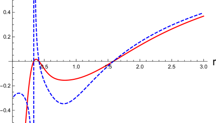
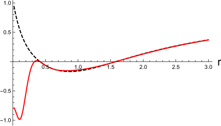
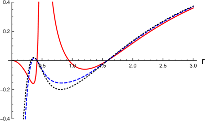
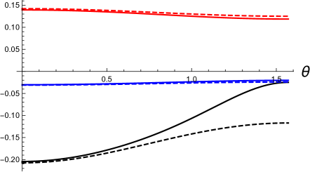
In Fig. 1, we show a few examples of the disformed Kerr-Newman solution in the vicinity of the black hole event horizon. The metric functions in the disformed Kerr-Newmans solution are shown as the functions of . In the left panels, (the disformed Kerr-Newman solution, the red-solid curves) and (the disformed Kerr-Newman solution, the blue-dashed curves) are shown as the functions of . In the right panels, (the disformed Kerr-Newman solution, the red-solid curves) and (the Kerr-Newman solution, the black-dashed curves) are shown as the functions of . We choose and in the top and bottom panels, respectively, and set the other parameters to , , and in the units of .
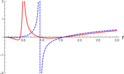
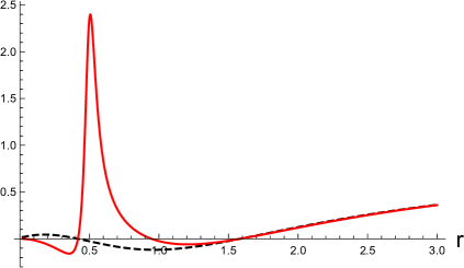
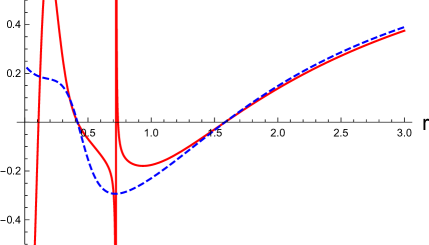
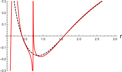
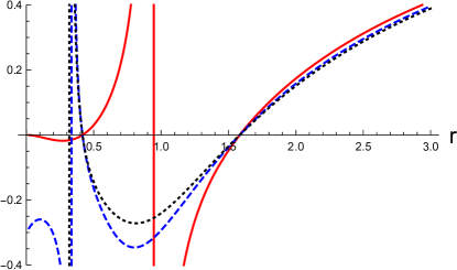
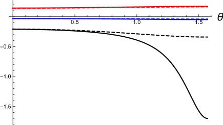
The same plots as Fig. 1 for the different angle are shown in Fig 2. In these examples, the black hole event horizon is located at in the units of irrespective of the polar angle , and there are several singularities at the finite values of inside the black hole event horizon. The value of does not affect the position of the event horizon, which remains the same as that in the original solution before the disformal transformation. Outside the event horizon, the difference between the disformed Kerr-Newman and original Kerr-Newman solutions quickly approaches zero.
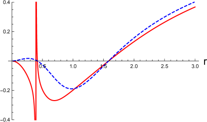
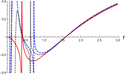
In Fig, 3, and (the disformed Kerr-Newman solution, see Eq. (106)) for several different polar angles with the fixed other parameters are shown. In the left panels, (the disformed Kerr-Newman solution) is shown as the function of for by the red-solid, blue-dashed, and black-dotted curves, respectively. In the right panels, (the disformed Kerr-Newman solution) is shown as the function of for by the red-solid, blue-dashed, and black-dotted curves, respectively. We choose and in the top and bottom panels, respectively, and set the other parameters to and in the units of . In these examples, the black hole event horizon is located at in the units of , irrespective of .
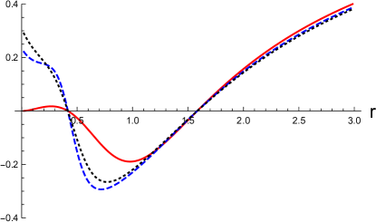
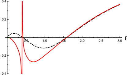
In Fig. 4, the angular dependence of the metric functions in the Kerr-Newman and disformed Kerr-Newman solutions is shown as the function of . We note that the horizontal axis denotes between and , as the metric components are symmetric across the equatorial plane . In the left panels, (the disformed Kerr-Newman solution, the solid curves) and (the Kerr-Newman solution, the dashed curves) are shown as the functions of respectively. In the right panels, (the disformed Kerr-Newman solution, the solid curves) and (the Kerr-Newman solution, the dashed curves) are shown as the functions of . The red, blue, and black curves correspond to the positions of in the units of , respectively. For the disformed Kerr-Newman solution, we choose and in the top and bottom panels, respectively, and set the other parameters to and in the units of .
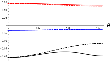
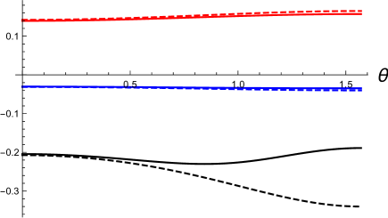
In both Figs. 3 and 4, the black hole event horizon is located at in the units of . In these examples, the singularities are hidden by the event horizon. We find that the position of the event horizon does not depend on the polar angle , and the spacetime structure inside the horizon and the position of the singularities depend on . The deviation from the Kerr-Newman solution is more significant in the vicinity of the equatorial plane and for smaller values of .
The leading order contributions to the disformed Kerr-Newman metric in the large distance limit are given by
| (107) |
Thus, for a generic dimensionless spin parameter , the leading order disformal corrections, which depend on , appear in the frame-dragging component at , which is suppressed by the factor of in comparison with the leading order Kerr term . We note in the case that is given by some positive powers of and , the disformal correction to the frame-dragging component is suppressed by inverse powers of higher than . Thus, the disformed black hole solution may be able to be distinguished from the original Kerr-Newman solution only via the direct measurements such as black hole shadows. The detailed studies of the observational properties of the disformed Kerr-Newman solution will be left for future work.
VIII The disformed solutions in the Einstein-conformally coupled scalar field theory
Finally, as the example of scalar-tensor theories without the shift symmetry, we consider the Einstein-conformally coupled scalar field theory
| (108) |
There exists the BBMB solution Bocharova et al. (1970); Bekenstein (1975) with the leading order slow rotation corrections given by Eqs. (16) and (21) with
| (109) |
and
| (110) |
where we set the constant term to be zero, so that the disformed spacetime is asymptotically flat. In the large distance limit ,
| (111) |
Thus, the leading term of agrees with Eq. (97) with , and the difference from the slow rotation limit of the Kerr solution ( in the case of Eq. (97)) appears at .
We consider the disformal transformation (41) where and are the functions only of or , separately. First, in the case of and where and are constants, the disformed BBMB solution with the leading order slow rotation corrections is given by
| (112) | |||||
As , the metric solution asymptotically approaches the flat Minkowski spacetime. Second, in the case of and where and are constant, the disformed BBMB solution with the leading order slow rotation corrections is given by
| (113) | |||||
As , besides the overall conformal factor , the metric approaches , where . Thus the deficit solid angle is given by .
In both the cases of Eqs. (112) and (113), up to , the degenerate black hole event horizon is located at . Thus, at , the disformal transformation does not modify the position of the black hole event horizon, since the character of the scalar field is spacelike. This confirms the general properties of the disformed black hole solutions within the slow rotation approximation in the scalar-tensor theories without the shift symmetry discussed in Sec. III.3. The physical properties of the disformed solution crucially depend on the choice of the functions and . As discussed in Sec. III.3, the circularity conditions (6) are always satisfied even beyond the slow rotation approximation. The scalar field in the disformed BBMB solution blows up at the event horizon as in the case of the original solution, irrespective of and .
IX Conclusions
We have investigated the disformal transformation of stationary and axisymmetric solutions in a broad class of the vector-tensor and scalar-tensor theories. We have started from the most general form of the stationary and axisymmetric solutions obeying the integrability conditions (5), for which the circularity conditions (6) have to be satisfied. We have shown that after the disformal transformations (22) and (35) in the vector-tensor theories without and with the gauge symmetry, respectively, and the resultant stationary and axisymmetric solutions (25) and (37) in general do not satisfy the circularity conditions (6), except for the cases that Eqs. (27) and (38) are satisfied.
Using the fact that a solution in a class of the vector-tensor theories without the gauge symmetry and with the vanishing field strength , after the replacement of and the integration of it, is uniquely mapped to that in the corresponding class of the shift-symmetric scalar-tensor theories with the scalar field , we have shown that in the shift-symmetric scalar-tensor theories the general form of the scalar field in the stationary and axisymmetric spacetime is given by Eq. (13), and the disformed stationary and axisymmetric metric (42) does not satisfy the circularity conditions for or , namely, in the case that the scalar field depends on the time or the azimuthal angle . On the other hand, in the scalar-tensor theories without the shift symmetry, the scalar field cannot depend on these coordinates and then the disformed stationary and axisymmetric solution always satisfies the circularity conditions. Thus, any violation of the circularity conditions may indicate the existence of the vector field or the scalar field with the unbroken shift symmetry, irrespective of the detailed structure of the action of the vector-tensor or scalar-tensor theories.
Second, as the concrete examples, we have considered the generalized Proca theory with the nonminimal coupling to the Einstein tensor (50). As the particular case, a solution with the vanishing field strength , after the replacement of and the integration of it, could be mapped to that in the shift-symmetric scalar-tensor theory with the nonminimal derivative coupling to the Einstein tensor (51). We have started from the reference static and spherically symmetric solutions in these theories and then derived the leading order slow rotation corrections to the metric functions and the vector or scalar field. Up to the leading order slow rotation corrections to the reference solutions, in the generalized Proca theory (50) we have obtained the nonzero values of the component of the metric and the azimuthal component of the vector field, while in the shift-symmetric scalar-tensor theory (51) the scalar field remains the same as that in the static and spherically symmetric solution (21). The disformal transformations of Eqs. (22) and (35) induced the and components of the metric and the component of the vector field, up to the first order of the slow rotation approximation, respectively, where the former could be eliminated by the redefinition of the timelike coordinate (32).
After the disformal transformation (22), the generalized Proca theory is mapped to a class of the extended vector-tensor theories without the Ostrogradsky ghosts Kimura et al. (2017). At the zeroth order of the slow rotation approximation, via the disformal transformation the stealth Schwarzschild solution obtained for any value of the coupling parameter and the charged stealth Schwarzschild solution obtained for the particular value of the coupling constant are mapped to the stealth Schwarzschild solution and the RN solution with the maximally two horizons, respectively, where the position of the black hole event horizon was modified. In the near-horizon limit, the vector field expressed in terms of the new time coordinate defined in the disformed frame (32) is proportional to the null coordinates which are regular at the future and past event horizons, respectively. Thus, the positive and negative branch solutions of the vector field are regular at the future and past event horizons, respectively, and the disformal transformation does not modify the essential properties of the vector field from the original one Minamitsuji (2016). The similar properties could also be verified for the Schwarzschild-(anti-) de Sitter solutions and the charged Schwarzschuld- (anti-) de Sitter solutions, where the vector field written in terms of the time coordinate defined in the disformed frame is regular at either the future or past event horizon (and at either the past or future cosmological horizon, if the cosmological horizons exist).
In the case of the disformal transformation with the gauge invariance (35), we showed at the leading order of the slow rotation approximation, the disformal transformation does not modify the position of the black hole event horizon, in contrast to the case of the disformal transformation without the gauge symmetry (22). We have explicitly confirmed this for the reference RN solution. We also obtained the disformal transformation of the Kerr-Newman solution for an arbitrary dimensionless spin parameter. We then showed that the position of the black hole event horizon is not modified by the disformal transformation, although the too large disformal contribution leads to singularities at the finite values of the radial coordinate. Moreover, we saw that in the large distance limit the leading disformal contribution appears at the frame-dragging component of the disformed Kerr-Newman metric, but is suppressed by the inverse powers of the radial coordinate.
Finally, as the example of the scalar-tensor theories without the shift symmetry, we have considered the disformal transformation of the BBMB solution (109) with the leading order slow rotation corrections (110). We confirmed that the disformed BBMB solution with the slow rotation corrections satisfies the circularity conditions, which is the general property of the disformed stationary and axisymmetric solutions in the scalar-tensor theories without the shift symmetry.
Before closing this paper, we would like to emphasize again that as long as the disformal transformation is invertible, there should be always one-to-one correspondence between the original theory and the theory obtained after the disformal transformation, and they should share the equivalent solution space, in the case that the contribution of matter is absent Zumalacárregui and García-Bellido (2014); Ben Achour et al. (2016a); Kimura et al. (2017); Gumrukcuoglu and Namba (2020). Even in the case that the theory obtained via the disformal transformation is apparently higher derivative while the original theory gives rise to the second-order Euler-Lagrange equations, the higher-derivative Euler-Lagrange equations in the disformed theory should be degenerate and reduce to the second-order system after the suitable redefinition of the variables. In such a case, the two theories should be just the two different mathematical descriptions of the same theory and have no physical difference at all. Hence, the order of the disformal transformation and the variation of the action should be able to be exchanged, and the disformed solutions should always satisfy the Euler-Lagrange equations obtained by varying the action of the theory derived via the disformal transformation. We note that since we assumed that matter is minimally coupled to the metric in each frame, we have regarded the two theories as the physically independent ones; e.g., the trajectories of particles freely falling into a black hole are different, although we have neglected the contribution of matter in deriving the solutions.
In Appendix B, we have explicitly demonstrated that the disformal transformation of the asymptotically flat solutions discussed in Sec. IV satisfies the Euler-Lagrange equations of the extended vector-tensor theories derived via the disformal transformation of the generalized Proca theories (50). The same conclusions should be obtained for the vector disformal transformation with the gauge symmetry and the scalar disformal transformation without the shift symmetry, as long as these disformal transformations are invertible.
On the other hand, our main purpose was to show to which a new metric a disformal transformation maps a general stationary and axisymmetric solution satisfying the circularity conditions, assuming that the transformation is invertible. The explicit examples shown in Secs. IV-VIII were just to confirm the general properties of the disformed solution mentioned in Sec. III. Our main result is that if the future observations could measure any violation of the circularity conditions, it would indicate the existence of the vector field without the symmetry or the scalar field with the shift symmetry in the vicinity of the black hole, irrespective of the detailed structure of the action of the scalar-tensor or vector-tensor theories obtained via the disformal transformation. Therefore, in this paper, instead of the derivation of the explicit action of the scalar-tensor and vector-tensor theories obtained via the disformal transformations, we have focused on the disformal transformations at the level of the solutions.
There are several issues left for future studies. First, in the case that the disformed stationary and axisymmetric solutions do not satisfy the circularity conditions, it will be important to see the consequences on astrophysical phenomena and the implications on observations such as black hole shadows and gravitational waves (see Refs. Psaltis et al. (2020); Psaltis (2019) for the constraints on the deviations from the Kerr solution with the latest data of black hole shadows by the Event Horizon Telescope). Second, it will also be important to explore more explicit stationary and axisymmetric solutions with the nontrivial field profiles of the scalar or vector field beyond the slow rotation and the properties of their disformed solutions. We hope to come back to these issues in our future publications.
Acknowledgements.
M.M. was supported by the Portuguese national fund through the Fundação para a Ciência e a Tecnologia in the scope of the framework of the Decree-Law 57/2016 of August 29, changed by Law 57/2017 of July 19, and the CENTRA through the Project No. UIDB/00099/2020.Appendix A The disformed Kerr solution
In this appendix, we review the disformed Kerr solution obtained from the stealth Kerr solution in the DHOST theories Anson et al. (2020); Ben Achour et al. (2020b).
In the coordinate system (8), the Kerr solution in the Boyer–Lindquist form is described by Eqs. (VII)–(100) with and . We assume that the scalar field does not depend on and ,
| (114) |
and consider the scalar disformal transformation (41) with and . The disformed solution is then given by
| (115) |
In a subclass of the Class-Ia DHOST theories Langlois and Noui (2016); Ben Achour et al. (2016a, b); Langlois (2019), the stealth Kerr solution was obtained Charmousis et al. (2019); Babichev et al. (2020); Anson et al. (2020); Ben Achour et al. (2020b), where is given by
| (116) |
for which the kinetic term of the scalar field (14) is given by .
The disformed metric (115) then reduces to
| (117) | |||||
Introducing the rescaled time coordinate and mass, and , respectively,
| (118) | |||||
which does not reduce to the circular form of Eq. (8) because of the nonzero component of . The physical properties of the disformed Kerr metric, e.g., the position of the black hole event horizon, were discussed in Refs. Anson et al. (2020); Ben Achour et al. (2020b).
Appendix B The solutions of the equations of motion in the disformed generalized Proca theory
As long as the disformal transformation is invertible, there should be one-to-one correspondence between the original theory and the theory obtained after the disformal transformation, and they should share the equivalent solution space, in the case that the contribution of matter is absent. Even in the case that the theory obtained via the disformal transformation is apparently higher derivative while the original theory gives rise to the second-order Euler-Lagrange equations, the higher-derivative Euler-Lagrange equations in the disformed theory should be degenerate and reduce to the second-order system after the suitable redefinition of the variables. The two theories should be the two different mathematical descriptions of the equivalent theory, as long as the contribution of matter is absent. Thus, the order of the disformal transformation and the variation of the action should be able to be exchanged, and the disformed solutions should satisfy the Euler-Lagrange equations obtained by varying the action of the theory derived via the disformal transformation.
In this appendix, we demonstrate that the disformed asymptotically flat solutions discussed in Sec. IV satisfy the Euler-Lagrange equations obtained by varying the action of the extended vector-tensor theory derived via the disformal transformation (22) of the generalized Proca theory (50) with , as long as the disformal transformation is invertible. Here, we employ the conventions employed in Ref. Kimura et al. (2017), where the correspondence with the conventions in the main text (see Eqs. (22) and (125)) is given by
| (119) |
We consider the generalized Proca theory (50) with , rewritten in terms of the new conventions as
| (120) |
where we attach “bar” to the quantities defined in the frame before the disformal transformation (see Eq. (125)). Following the general formulation of the generalized Proca theory Heisenberg (2014); De Felice et al. (2016), the theory (120) is given by the choice of
| (121) |
and the others to be zero, where . Moreover, following the general form of the extended vector-tensor theories Kimura et al. (2017), the theory (120) can be described by
| (122) |
with
and with the replacement to the barred quantities (, , and ), where the coefficients in are given by
| (124) |
We consider the disformal transformation from the frame to the new frame , given by
| (125) |
which maps the generalized Proca theory written in terms of to a class of the extended vector-tensor theories without the Ostrogradsky ghosts Kimura et al. (2017), given by
| (126) |
where is defined in Eq. (B) with the coefficients related to () by
| (127) | |||||
| (128) | |||||
| (129) | |||||
| (130) | |||||
| (131) | |||||
| (132) |
The inverse transformation to Eq. (125) is given by
| (133) |
where , respectively. For simplicity, we assume the constant disformal transformation
| (134) |
and the invertibility of the transformation .
We consider the static and spherically symmetric Ansatz for the metric and the vector field
| (135) | |||||
| (136) |
Plugging the Ansatz (135)-(136) into the action (126) and varying it with respect to , , , and , we obtain a set of the four independent Euler-Lagrangian equations.
B.1 On the disformal transformation of the stealth Schwarzschild solution
For our purpose, we impose the further simplification of and (and hence ), and hence
| (137) |
We also assume the proportionality of and , with being a constant. With these assumptions, the Euler-Lagrange equations with respect to and reduce to the first-order degenerate equation of ,
| (138) |
whose solution is given by the form of
| (139) |
where denotes the integration constant. In order to avoid the appearance of the deficit solid angle, we impose the constant part of to be unity, which fixes
| (140) |
Eq. (139) with Eq. (140) also satisfies the Euler-Lagrange equations for and . Thus, all the Euler-Lagrange equations are satisfied. In this way, we finally obtain the solution for the metric and the vector field, respectively, given by
| (141) |
and
| (142) |
The solution (141)-(142) is equivalent to that obtained after the disformed stealth Schwarzschild solution given by Eqs. (55)-(57) obtained in Sec. IV.1, after the replacement of , , , , and .
B.2 On the disformal transformation of the charged stealth Schwarzschild solution
Following the same procedure, we can also confirm that the disformal transformation of the charged stealth Schwarzschild black hole solution discussed in Sec. IV.2 is also the solution of the extended vector-tensor theory (126) derived via the disformal transformation.
We impose the simplification of and with and being constants, and hence
| (143) |
Again, we assume the proportionality of and , with being a constant. With these assumptions, the Euler-Lagrange equations with respect to and reduce to the first-order degenerate equation of , whose solution is given by
| (144) | |||||
where denotes the integration constant. In order to avoid the appearance of the deficit solid angle, we impose the constant part of to be unity, which fixes as Eq. (140).
Substituting Eq. (144) with Eq. (140) into the Euler-Lagrange equations for and results in the degenerate algebraic equation
Here, we choose the branch
| (146) |
Then, all the Euler-Lagrange equations are satisfied, and the solution for the metric and vector field is explicitly given by
| (147) | |||||
and
| (148) |
which agree with Eq. (64)-(65) after the replacement of , , , , and .
These examples demonstrated that the disformed solutions satisfy the Euler-Lagrange equations obtained by varying the the action of the vector-tensor theories derived via the disformal transformation of the original theory, as long as the disformal transformation is invertible. The same conclusion should be obtained for the scalar disformal transformation and the vector disformal transformation with the gauge symmetry, given by Eqs. (41) and (35), respectively, as long as these disformal transformations are invertible.
Appendix C The stationary and axisymmetric solutions and circularity conditions
In this appendix, we review the conditions under which the most general stationary and axisymmetric spacetime Eq. (4) with the two commuting Killing vector fields and reduce to the form of Eq. (7) with the integrable two-surfaces orthogonal to and .
There is the theorem stating that the two-surfaces orthogonal to and are integrable, if and satisfy (see e.g., Refs. Kundt and Trumper (1966); Carter (1969); Wald (1984))
- (i)
-
Each of and vanishes at least at a point in the spacetime.
- (ii)
Frobenius’s theorem states that the necessary and sufficient conditions for integrability are given by Eq. (5), which we recapitulate here
| (150) |
or equivalently,
| (151) |
where , , and denotes the volume element.
Here, we confirm that the assumptions (i) and (ii) are necessary for the integrability conditions (5). First, the assumption (i) ensures that each of the products and vanishes at least at a point in the spacetime (e.g., on the symmetry axis). They vanish in the entire spacetime, if
| (152) |
Since , the diffeomorphism group generated by leaves invariant, and similarly, the diffeomorphism group generated by does invariant. Thus, any tensor constructed by and their derivatives is invariant under , and hence is invariant under , i.e., . Similarly, any tensor constructed by and their derivatives is also invariant under , and hence is invariant under , i.e., . Thus, Eq. (152) reduces to
| (153) |
After some algebra, we obtain
| (154) |
Then, under the assumption (ii), i.e., Eq. (6),
| (155) |
which ensures that Eq. (151) holds in the entire spacetime and hence the existence of the integrable orthogonal two-surfaces. This ensures that the circularity conditions (6) are necessary for the integrability conditions (5).
For the general stationary and axisymmetric spacetime metric (4), the possible terms which violate the circularity conditions (6) are given by the components of the Ricci tensor , , , and , and all these components of the Ricci tensor vanish, if the metric form is given by Eq. (7) or (8). In general relativity, the condition (6) holds in the vacuum spacetime where with being constant, or in the spacetime filled with the perfect fluids with the four-velocities spanned by the two Killing vector fields and , with and being constants. On the other hand, in the other gravitational theories with the nontrivial scalar or vector field degrees of freedom, the components does not necessarily vanish even in the vacuum spacetimes (or in the spacetime with the perfect fluids) and the circularity conditions (6) may not hold.
References
- Schwarzschild (1917) K. Schwarzschild, Sitzungsberichte der Koniglich Preussischen Akademie der Wissenschaften. 7, 189 (1917).
- Reissner (1916) H. Reissner, Annalen der Physik (in German) 50, 106 (1916).
- Nordstrom (1918) G. Nordstrom, Verhandl. Koninkl. Ned. Akad. Wetenschap., Afdel. Natuurk., Amsterdam 26, 1201 (1918).
- Kerr (1963) R. P. Kerr, Phys. Rev. Lett. 11, 237 (1963).
- Newman et al. (1965) E. T. Newman, R. Couch, K. Chinnapared, A. Exton, A. Prakash, and R. Torrence, J. Math. Phys. 6, 918 (1965).
- Israel (1967) W. Israel, Phys. Rev. 164, 1776 (1967).
- Israel (1968) W. Israel, Commun. Math. Phys. 8, 245 (1968).
- Carter (1971) B. Carter, Phys. Rev. Lett. 26, 331 (1971).
- Herdeiro and Radu (2015) C. A. R. Herdeiro and E. Radu, Proceedings, 7th Black Holes Workshop 2014, Int. J. Mod. Phys. D24, 1542014 (2015), arXiv:1504.08209 [gr-qc] .
- Ruffini and Wheeler (1971) R. Ruffini and J. A. Wheeler, Phys. Today 24, 30 (1971).
- Hawking (1972a) S. Hawking, Commun. Math. Phys. 25, 152 (1972a).
- Bekenstein (1972a) J. Bekenstein, Phys. Rev. D 5, 2403 (1972a).
- Bekenstein (1972b) J. Bekenstein, Phys. Rev. Lett. 28, 452 (1972b).
- Hawking (1972b) S. Hawking, Commun. Math. Phys. 25, 167 (1972b).
- Bekenstein (1995) J. Bekenstein, Phys. Rev. D 51, 6608 (1995).
- Sotiriou and Faraoni (2012) T. P. Sotiriou and V. Faraoni, Phys. Rev. Lett. 108, 081103 (2012), arXiv:1109.6324 [gr-qc] .
- Hui and Nicolis (2013) L. Hui and A. Nicolis, Phys. Rev. Lett. 110, 241104 (2013), arXiv:1202.1296 [hep-th] .
- Babichev et al. (2017a) E. Babichev, C. Charmousis, and A. Lehebel, JCAP 04, 027 (2017a), arXiv:1702.01938 [gr-qc] .
- Graham and Jha (2014) A. A. H. Graham and R. Jha, Phys. Rev. D 89, 084056 (2014), [Erratum: Phys.Rev.D 92, 069901 (2015)], arXiv:1401.8203 [gr-qc] .
- Bocharova et al. (1970) N. Bocharova, K. Bronnikov, and V. Melnikov, Vestn. Mosk. Univ. Ser. III Fiz. Astron. , 706 (1970).
- Bekenstein (1975) J. Bekenstein, Annals Phys. 91, 75 (1975).
- Kanti et al. (1996) P. Kanti, N. E. Mavromatos, J. Rizos, K. Tamvakis, and E. Winstanley, Phys. Rev. D54, 5049 (1996), arXiv:hep-th/9511071 [hep-th] .
- Ayzenberg and Yunes (2014) D. Ayzenberg and N. Yunes, Phys. Rev. D90, 044066 (2014), [Erratum: Phys. Rev.D91,no.6,069905(2015)], arXiv:1405.2133 [gr-qc] .
- Alexeev and Pomazanov (1997) S. O. Alexeev and M. V. Pomazanov, Phys. Rev. D55, 2110 (1997), arXiv:hep-th/9605106 [hep-th] .
- Torii et al. (1997) T. Torii, H. Yajima, and K.-i. Maeda, Phys. Rev. D55, 739 (1997), arXiv:gr-qc/9606034 [gr-qc] .
- Kanti et al. (1998) P. Kanti, N. E. Mavromatos, J. Rizos, K. Tamvakis, and E. Winstanley, Phys. Rev. D57, 6255 (1998), arXiv:hep-th/9703192 [hep-th] .
- Guo et al. (2008) Z.-K. Guo, N. Ohta, and T. Torii, Prog. Theor. Phys. 120, 581 (2008), arXiv:0806.2481 [gr-qc] .
- Babichev and Charmousis (2014) E. Babichev and C. Charmousis, JHEP 1408, 106 (2014), arXiv:1312.3204 [gr-qc] .
- Appleby (2015) S. Appleby, JCAP 05, 009 (2015), arXiv:1503.06768 [gr-qc] .
- Babichev et al. (2016) E. Babichev, C. Charmousis, and A. Lehebel, Class. Quant. Grav. 33, 154002 (2016), arXiv:1604.06402 [gr-qc] .
- Rinaldi (2012) M. Rinaldi, Phys. Rev. D86, 084048 (2012), arXiv:1208.0103 [gr-qc] .
- Anabalon et al. (2014) A. Anabalon, A. Cisterna, and J. Oliva, Phys. Rev. D89, 084050 (2014), arXiv:1312.3597 [gr-qc] .
- Minamitsuji (2014) M. Minamitsuji, Phys. Rev. D89, 064017 (2014), arXiv:1312.3759 [gr-qc] .
- Babichev et al. (2017b) E. Babichev, C. Charmousis, and A. Lehebel, JCAP 04, 027 (2017b), arXiv:1702.01938 [gr-qc] .
- Babichev et al. (2018) E. Babichev, C. Charmousis, G. Esposito-Farese, and A. Lehebel, Phys. Rev. Lett. 120, 241101 (2018), arXiv:1712.04398 [gr-qc] .
- Ben Achour and Liu (2019) J. Ben Achour and H. Liu, Phys. Rev. D 99, 064042 (2019), arXiv:1811.05369 [gr-qc] .
- Motohashi and Minamitsuji (2019) H. Motohashi and M. Minamitsuji, Phys. Rev. D 99, 064040 (2019), arXiv:1901.04658 [gr-qc] .
- Minamitsuji and Edholm (2019) M. Minamitsuji and J. Edholm, Phys. Rev. D 100, 044053 (2019), arXiv:1907.02072 [gr-qc] .
- Ben Achour et al. (2020a) J. Ben Achour, H. Liu, and S. Mukohyama, JCAP 02, 023 (2020a), arXiv:1910.11017 [gr-qc] .
- Minamitsuji and Edholm (2020) M. Minamitsuji and J. Edholm, Phys. Rev. D 101, 044034 (2020), arXiv:1912.01744 [gr-qc] .
- Sotiriou and Zhou (2014a) T. P. Sotiriou and S.-Y. Zhou, Phys. Rev. Lett. 112, 251102 (2014a), arXiv:1312.3622 [gr-qc] .
- Sotiriou and Zhou (2014b) T. P. Sotiriou and S.-Y. Zhou, Phys. Rev. D 90, 124063 (2014b), arXiv:1408.1698 [gr-qc] .
- Chagoya et al. (2016) J. Chagoya, G. Niz, and G. Tasinato, Class. Quant. Grav. 33, 175007 (2016), arXiv:1602.08697 [hep-th] .
- Minamitsuji (2016) M. Minamitsuji, Phys. Rev. D 94, 084039 (2016), arXiv:1607.06278 [gr-qc] .
- Babichev et al. (2017c) E. Babichev, C. Charmousis, and M. Hassaine, JHEP 05, 114 (2017c), arXiv:1703.07676 [gr-qc] .
- Heisenberg et al. (2017a) L. Heisenberg, R. Kase, M. Minamitsuji, and S. Tsujikawa, Phys. Rev. D 96, 084049 (2017a), arXiv:1705.09662 [gr-qc] .
- Heisenberg et al. (2017b) L. Heisenberg, R. Kase, M. Minamitsuji, and S. Tsujikawa, JCAP 08, 024 (2017b), arXiv:1706.05115 [gr-qc] .
- Hartle (1967) J. B. Hartle, Astrophys. J. 150, 1005 (1967).
- Hartle and Thorne (1968) J. B. Hartle and K. S. Thorne, Astrophys.J. 153, 807 (1968).
- Pani and Cardoso (2009) P. Pani and V. Cardoso, Phys. Rev. D79, 084031 (2009), arXiv:0902.1569 [gr-qc] .
- Maselli et al. (2015) A. Maselli, H. O. Silva, M. Minamitsuji, and E. Berti, Phys. Rev. D92, 104049 (2015), arXiv:1508.03044 [gr-qc] .
- Kleihaus et al. (2011) B. Kleihaus, J. Kunz, and E. Radu, Phys. Rev. Lett. 106, 151104 (2011), arXiv:1101.2868 [gr-qc] .
- Kleihaus et al. (2016) B. Kleihaus, J. Kunz, S. Mojica, and E. Radu, Phys. Rev. D93, 044047 (2016), arXiv:1511.05513 [gr-qc] .
- Charmousis et al. (2019) C. Charmousis, M. Crisostomi, R. Gregory, and N. Stergioulas, Phys. Rev. D 100, 084020 (2019), arXiv:1903.05519 [hep-th] .
- Babichev et al. (2020) E. Babichev, C. Charmousis, A. Cisterna, and M. Hassaine, JCAP 06, 049 (2020), arXiv:2004.00597 [hep-th] .
- Anson et al. (2020) T. Anson, E. Babichev, C. Charmousis, and M. Hassaine, (2020), arXiv:2006.06461 [gr-qc] .
- Ben Achour et al. (2020b) J. Ben Achour, H. Liu, H. Motohashi, S. Mukohyama, and K. Noui, (2020b), arXiv:2006.07245 [gr-qc] .
- Delgado et al. (2020) J. F. Delgado, C. A. Herdeiro, and E. Radu, JHEP 04, 180 (2020), arXiv:2002.05012 [gr-qc] .
- Herdeiro and Radu (2014) C. A. R. Herdeiro and E. Radu, Phys. Rev. Lett. 112, 221101 (2014), arXiv:1403.2757 [gr-qc] .
- Herdeiro et al. (2016) C. Herdeiro, E. Radu, and H. Runarsson, Class. Quant. Grav. 33, 154001 (2016), arXiv:1603.02687 [gr-qc] .
- Bekenstein (1993) J. D. Bekenstein, Phys. Rev. D48, 3641 (1993), arXiv:gr-qc/9211017 [gr-qc] .
- Zumalacárregui and García-Bellido (2014) M. Zumalacárregui and J. García-Bellido, Phys. Rev. D89, 064046 (2014), arXiv:1308.4685 [gr-qc] .
- Liberati (2013) S. Liberati, Class.Quant.Grav. 30, 133001 (2013), arXiv:1304.5795 [gr-qc] .
- Kimura et al. (2017) R. Kimura, A. Naruko, and D. Yoshida, JCAP 1701, 002 (2017), arXiv:1608.07066 [gr-qc] .
- Domènech et al. (2018) G. Domènech, S. Mukohyama, R. Namba, and V. Papadopoulos, Phys. Rev. D 98, 064037 (2018), arXiv:1807.06048 [gr-qc] .
- Gumrukcuoglu and Namba (2020) A. E. Gumrukcuoglu and R. Namba, Phys. Rev. D 100, 124064 (2020), arXiv:1907.12292 [hep-th] .
- De Felice and Naruko (2020) A. De Felice and A. Naruko, Phys. Rev. D 101, 084044 (2020), arXiv:1911.10960 [gr-qc] .
- Woodard (2015) R. P. Woodard, Scholarpedia 10, 32243 (2015), arXiv:1506.02210 [hep-th] .
- Langlois and Noui (2016) D. Langlois and K. Noui, JCAP 1602, 034 (2016), arXiv:1510.06930 [gr-qc] .
- Ben Achour et al. (2016a) J. Ben Achour, D. Langlois, and K. Noui, Phys. Rev. D93, 124005 (2016a), arXiv:1602.08398 [gr-qc] .
- Ben Achour et al. (2016b) J. Ben Achour, M. Crisostomi, K. Koyama, D. Langlois, K. Noui, and G. Tasinato, JHEP 12, 100 (2016b), arXiv:1608.08135 [hep-th] .
- Langlois (2019) D. Langlois, Int. J. Mod. Phys. D 28, 1942006 (2019), arXiv:1811.06271 [gr-qc] .
- Nakashi and Kimura (2020) K. Nakashi and M. Kimura, (2020), arXiv:2008.04003 [gr-qc] .
- Kundt and Trumper (1966) W. Kundt and M. Trumper, Z. Phys. 192, 419 (1966).
- Carter (1969) B. Carter, J. Math. Phys. 10, 70 (1969).
- Wald (1984) R. M. Wald, General Relativity (University of Chicago Press, Chicago, 1984).
- Bambi (2012a) C. Bambi, Phys. Rev. D 85, 043001 (2012a), arXiv:1112.4663 [gr-qc] .
- Bambi (2012b) C. Bambi, Phys. Rev. D 86, 123013 (2012b), arXiv:1204.6395 [gr-qc] .
- Konoplya and Zhidenko (2013) R. Konoplya and A. Zhidenko, Phys. Rev. D 87, 024044 (2013), arXiv:1210.8430 [gr-qc] .
- Glampedakis and Babak (2006) K. Glampedakis and S. Babak, Class.Quant.Grav. 23, 4167 (2006), arXiv:gr-qc/0510057 [gr-qc] .
- Johannsen and Psaltis (2010a) T. Johannsen and D. Psaltis, Astrophys. J. 716, 187 (2010a), arXiv:1003.3415 [astro-ph.HE] .
- Johannsen and Psaltis (2010b) T. Johannsen and D. Psaltis, Astrophys. J. 718, 446 (2010b), arXiv:1005.1931 [astro-ph.HE] .
- Vigeland et al. (2011) S. Vigeland, N. Yunes, and L. Stein, Phys.Rev. D83, 104027 (2011), arXiv:1102.3706 [gr-qc] .
- Medeiros et al. (2020) L. Medeiros, D. Psaltis, and F. Özel, Astrophys. J. 896, 7 (2020), arXiv:1907.12575 [astro-ph.HE] .
- Heisenberg (2014) L. Heisenberg, JCAP 05, 015 (2014), arXiv:1402.7026 [hep-th] .
- Tasinato (2014) G. Tasinato, JHEP 04, 067 (2014), arXiv:1402.6450 [hep-th] .
- De Felice et al. (2016) A. De Felice, L. Heisenberg, R. Kase, S. Tsujikawa, Y.-l. Zhang, and G.-B. Zhao, Phys.Rev.D 93, 104016 (2016), arXiv:1602.00371 [gr-qc] .
- Horndeski (1974) G. W. Horndeski, Int.J.Theor.Phys. 10, 363 (1974).
- Deffayet et al. (2009) C. Deffayet, S. Deser, and G. Esposito-Farèse, Phys. Rev. D80, 064015 (2009), arXiv:0906.1967 [gr-qc] .
- Kobayashi et al. (2011) T. Kobayashi, M. Yamaguchi, and J. Yokoyama, Prog. Theor. Phys. 126, 511 (2011), arXiv:1105.5723 [hep-th] .
- Psaltis et al. (2020) D. Psaltis et al. (EHT), Phys. Rev. Lett. 125, 141104 (2020), arXiv:2010.01055 [gr-qc] .
- Psaltis (2019) D. Psaltis, Gen. Rel. Grav. 51, 137 (2019), arXiv:1806.09740 [astro-ph.HE] .