Disentangling Interpretable Factors with Supervised Independent Subspace Principal Component Analysis
Abstract
The success of machine learning models relies heavily on effectively representing high-dimensional data. However, ensuring data representations capture human-understandable concepts remains difficult, often requiring the incorporation of prior knowledge and decomposition of data into multiple subspaces. Traditional linear methods fall short in modeling more than one space, while more expressive deep learning approaches lack interpretability. Here, we introduce Supervised Independent Subspace Principal Component Analysis (sisPCA), a PCA extension designed for multi-subspace learning. Leveraging the Hilbert-Schmidt Independence Criterion (HSIC), sisPCA incorporates supervision and simultaneously ensures subspace disentanglement. We demonstrate sisPCA’s connections with autoencoders and regularized linear regression and showcase its ability to identify and separate hidden data structures through extensive applications, including breast cancer diagnosis from image features, learning aging-associated DNA methylation changes, and single-cell analysis of malaria infection. Our results reveal distinct functional pathways associated with malaria colonization, underscoring the essentiality of explainable representation in high-dimensional data analysis.
1 Introduction
High-dimensional data generated by complex biological mechanisms encapsulate an ensemble of patterns. A prime example is single-cell RNA sequencing (scRNA-seq) data (Fig. 1). These datasets measure the expression of tens of thousands of genes across potentially millions of cells, creating rich tapestries woven from interacting cellular pathways, gene dynamics, cell states, and inherent measurement noise. To unravel these patterns and reveal hidden relationships, it is necessary to decompose the data into meaningful, lower-dimensional subspaces.

Linear representation learning methods, such as Principal Component Analysis (PCA) (Hotelling, 1933) and Independent Component Analysis (ICA) (Comon, 1994), extract latent spaces from data using explainable linear transformations. These widely employed unsupervised tools learn a single latent space or a union of one-dimensional subspaces. Independent Subspace Analysis (ISA) extends ICA by extracting multidimensional components as independent subspaces (Cardoso, 1998). Yet, the unsupervised nature of these methods precludes knowledge integration, restricting their utility and sometimes even identifiability (Theis, 2006). In the context of Fig. 1, the representation learned without supervision fails to separate temporal variability from technical batch effects.
Conversely, recent advancements in deep generative models, especially semi-supervised approaches (Kingma et al., 2014), have shown promise in disentangling diverse latent spaces and retaining relevant information under supervision. However, challenges remain in ensuring subspace independence within a variational autoencoder (VAE). While models like -VAE (Higgins et al., 2016), HCV (Lopez et al., 2018) and biolord (Piran et al., 2024) attempt to address this, inference for deep generative models remains challenging and the learned representations are not interpretable.
To bridge the gap, we propose Supervised Independent Subspace Principal Component Analysis (sisPCA)111A Python implementation of sisPCA is available on GitHub at https://github.com/JiayuSuPKU/sispca (DOI 10.5281/zenodo.13932660). The repository also includes notebooks to reproduce results in this paper., an innovative method extending PCA to multiple subspaces. By incorporating the Hilbert-Schmidt Independence Criterion (HSIC), sisPCA effectively decomposes data into explainable independent subspaces that align with target supervision. It thus reconciles the simplicity and clarity of linear methods with the nuanced multi-space modeling capabilities of advanced generative models. In summary, our contributions include:
-
•
A multi-subspace extension of PCA for disentangling linear latent subspaces in high-dimensional data. We additionally show that supervising subspaces with a linear target kernel can be conceptualized as linear regression regularized akin to Zellner’s g-prior.
-
•
An efficient eigendecomposition-based alternating optimization algorithm to compute sisPCA subspaces. The learning process with linear kernels resembles matrix factorization, which may potentially benefit from desirable local geometric properties (Conjecture 3.1).
-
•
Demonstrated effectiveness and interpretability of sisPCA in various applications. This includes identifying diagnostic image features for breast cancer, dissecting aging signatures in human DNA methylation data, and unraveling time-independent transcriptomic changes in mouse liver cells upon malaria infection.
2 Background
2.1 Hilbert-Schmidt Independence Criterion (HSIC)
The Hilbert-Schmidt Independence Criterion (HSIC) serves as a methodology for testing the independence of two random variables and (Gretton et al., 2005a). It operates by embedding probability distributions into reproducing kernel Hilbert spaces (RKHS) and quantifying independence by distance between the joint distribution and the product of its marginals. Specifically, HSIC builds on the cross-covariance operator , which is a generalization of the cross-covariance matrix to infinite-dimensional RKHS (i.e., the feature spaces of and after transformation),
Here and are the RKHSs with feature maps and for and respectively. The tensor product operator maps to , such that The HSIC is then defined as,
where and are the orthogonal bases of and . and are independent if and only if . In practice, given a finite sample from the joint distribution , the empirical HSIC can be computed as,
where and are matrices of kernel evaluations over the samples in and in , and is the centering matrix defined as , with being the identity matrix.
2.2 Related work
The HSIC, as a non-parametric criterion for independence, has been effectively integrated into numerous representation learning models, especially for disentangling complex data structures. One of the earliest applications of HSIC is ICA (Comon, 1994), where the goal is to recover unmixed and statistically independent sources. Gretton et al. (2005a) showed that minimizing HSIC via gradient descent outperforms specialized linear ICA algorithms. Alternatively, HSIC can also be maximized to encode specific information in learning tasks. In supervised PCA (sPCA), HSIC is deployed to guide the identification of principal subspaces with maximum dependence on target variables (Barshan et al., 2011). More recently, Ma et al. (2020) used HSIC as a supervised learning objective for deep neural networks to bypass back-propagation, and Li et al. (2021) subsequently extend it to the context of self-supervised learning.
Our primary interest lies in extending these models to identify multiple subspaces, each representing independent, meaningful signatures. In this direction, Cao et al. (2015) suggested the inclusion of HSIC as a diversity term in multi-view subspace clustering, encouraging representations from different views to capture complementary information. Building on a similar idea, Lopez et al. (2018) incorporated HSIC-based regularization into VAE architectures to promote subspace separation. However, there has yet to be a linear multi-space model for more interpretable data decomposition.
The presented work is also related to contrastive representation learning, as introduced in Abid et al. (2018) and Abid and Zou (2019). Along this line of research, recent studies have also applied HSIC to regularize contrastive VAE subspaces (Tu et al., 2024; Qiu et al., 2023). See Appendix A for more discussions on connections and differences.
3 The sisPCA model
We introduce Supervised Independent Subspace Principal Component Analysis (sisPCA), a linear model for disentangling independent data variation (Fig. 2). The model’s linearity ensures explicit interpretability and enables regression-based extensions such as sparse feature selection. We formally discuss the connection between sisPCA and regularized linear regression in Section 3.2.

3.1 Problem formulation
As motivated in Fig. 1, given a dataset with observations and features and associated target variables , we aim to find separate subspace representations of the data with latent dimensions . Each subspace should maximize dependence with one target variable while minimizing dependence with other subspaces. For simplicity, we assume Euclidean space, and . Other types of data can be easily handled using appropriate kernels, which will be discussed later. The linear projection to the -th subspace is represented by the matrix , with being the data representation in this -th subspace. Similar to the concept of PCA loading, the projection depicts linear combinations of original features in and thus can be directly interpreted as feature importance scores.
Our overall objective is to find the set of subspace projections that solves
under some constraints. Here is a measure of dependence and penalizes overlapping subspaces. Using HSIC as the dependence measure, sisPCA solves the constrained optimization
| (1) | ||||
where and are kernels defined on the -th subspace and the -th target variable , respect. This formulation differs from kernel PCA, where in the first term of (1) the kernel is defined over rather than (the kernel extension of sisPCA will be discussed later).
In the special case where is linear for all subspaces, the optimization becomes
| (2) | ||||
The first term is the supervised PCA objective (Barshan et al., 2011). We can thus view the above formulation, termed sisPCA-linear, as an extension of supervised PCA to multiple subspaces with additional regularization for subspace independence (Fig. 2). It comes with an appealing property:
Remark 3.1.
We now examine the second HSIC term in (2). Consider two subspaces and with centered . The HSIC regularization is
This term equals zero if and only if and are orthogonal. While not convex in and jointly, the coupling of and solely through the matrix product indicates a well-behaved local geometry, as explored by Sun and Luo (2016). Indeed, it allows sisPCA-linear to benefit from theoretical insights on matrix factorization. For example, Ge et al. (2017) showed that for a quadratic function over the matrix — in our context — all local minima are also globally optimal under mild conditions achievable through proper regularization.
Returning to (2), we see that spurious local optima may only emerge from subspace imbalance in the first symmetry-breaking supervision term, where some subspaces may contribute more to the overall objective. This leads to the following conjecture on the optimization landscape of (2):
Conjecture 3.1
(informal): The sisPCA-linear objective (2) has no spurious local optima under balanced supervision, which is achievable through proper regularization; With unbalanced supervision, the global optima can still be recovered using local search algorithms following simple initialization based on the relative supervision strength of each subspace.
Intuitively, the balanced supervision condition is to ensure that the local optima induced by subspace symmetry and interchangeability are also global optima. For more discussions on the optimization landscape, the balance condition, and Conjecture 3.1, see Appendix C.
We now consider an iterative optimization approach to solve (2).
Remark 3.2.
The optimization problem in (2) can be solved via alternating optimization, where each iteration has an analytical update for each subspace.
Using basic matrix algebra, the objective of (2) simplifies to,
where and . Given the set , can be updated by maximizing , leading to the update , where are the columns of corresponding to the largest eigenvalues from the eigendecomposition .
The full optimization process is outlined in Algorithm 1, Appendix B. This procedure guarantees convergence to an optimum as the objective is bounded and non-decreasing in every iteration. We further implement an initialization step to find the path (subspace update order) towards the global optimum as proposed in Conjecture 3.1. Briefly, we compare subspace contributions to the supervision loss and prioritize updates for subspaces under stronger supervision.
While convenient, a zero HSIC regularization loss with a linear kernel in (2) does not guarantee independent subspaces. For strict independence, the subspace kernel in (1) needs to be universal (e.g., Gaussian). We refer to this as sisPCA-general and solve it using gradient descent (Algorithm 2, Appendix D). The naive implementation with a Gaussian kernel has complexity in contrast to with a linear kernel. See Appendix D for performance difference discussions.
Both sisPCA-linear and sisPCA-general are linear methods where measures direct contribution of original features to each subspace. Nevertheless, the sisPCA framework can be easily extended to incorporate nonlinear feature interactions, analogous to kernel PCA. See Appendix E.
3.2 Kernel selection for different target variables
The use of kernel independence measure in (1) allows sisPCA to accommodate various data types through flexible kernel choices for (data), (latent subspace), and (target).
For categorical variables (e.g., cancer types), we use the Dirac delta kernel,
It is also possible to use other general graph kernels for categorical variables with an intrinsic hierarchical structure, e.g., subtypes and stages (Smola and Kondor, 2003).
For continuous variables , we use the linear kernel
When is multivariate, the kernel is the sum of per-dimension kernels .
Remark 3.3.
In a nutshell, we show that sisPCA-linear can be viewed as approximating the target with . The particular regularization on corresponds to a zero-mean multivariate Gaussian prior, which is related to Zellner’s g-prior in Bayesian regression.
3.3 Learning an unknown subspace without supervision
In practical applications, a common goal would be to recover both subspaces linked to known attributes (supervised) and to unknown attributes (unsupervised) simultaneously. In sisPCA, this is achieved by setting the target kernel for the unknown subspace to the identity matrix (), corresponding to unsupervised PCA (Fig. 2). Section 4.1 provides an example of this process.
However, the absence of external supervision introduces a potential identifiability issue. As indicated in Appendix B eq. 4 each supervised subspace is driven by two forces to (1) align with the target and (2) capture major variations in the data. This dual objective can lead to scenarios where unknown attributes, ideally retained in the residual unsupervised subspace, being inadvertently presented in supervised subspaces. Fig. 8 in Appendix D gives an example where sisPCA-general fails.
4 Applications
Unless otherwise specified, in the following sections sisPCA refers to sisPCA-linear, where the objective (2) is solved using Algorithm 1. For baseline comparisons, we consider linear models including PCA and sPCA. While non-linear VAE counterparts such as HCV (Lopez et al., 2018) are included for quantitative performance benchmarking in Section 4.4, they are not considered for interpretability analyses due to their inherent complexity. The rationale and details for baseline selection are provided in Appendix F.
4.1 Recovering supervised and unsupervised subspaces in simulated data
We first consider learning latent subspaces associated with known and unknown attributes using simulated data. The dataset reflects a ground truth 6-dimensional latent space, comprising three distinct 2D subspaces (Fig. 3a): S1 with two Gaussian distributions, S2 with a noisy 2D grid and S3 with a ring structure. The defining manifold characteristics of S3 remain unknown to the model, representing the unsupervised component. These subspaces were concatenated and linearly projected to 20-dimensions using a matrix with entries uniformly distributed on .


Both unsupervised PCA (targeting S3) and supervised PCA (S1 and S2) subspaces capture structures heavily influenced by S2 (Fig. 3b and Fig. 11 in Appendix H), due to S2’s pronounced variations. In contrast, sisPCA markedly improves the disentanglement of these subspaces, especially the unsupervised S3 (Fig. 3c). Despite S2’s dominant influence, sisPCA isolates the effects of each subspace, resulting in clearer separation of the three independent signals. The two supervised subspaces S1 and S2 are distinctly characterized by patterns exclusively associated with the supervision attributes. In the unsupervised subspace S3, although Principal Component 2 (PC2) picks up some categorical information from S1, sisPCA successfully uncovers the underlying circular structure.
4.2 Learning diagnostic subspaces from breast cancer image features
We apply sisPCA to the Kaggle Breast Cancer Wisconsin Data222uciml/breast-cancer-wisconsin-data, CC BY-NC-SA 4.0 license. to demonstrate its utility in data compression and feature extraction. The dataset contains 569 samples with 30 summary features from breast mass imaging. Our goals are to (1) learn compressed subspaces for predicting disease status (‘Malignant’ or ‘Benign’, agnostic during training), and (2) understand the relationship between original features and how they contribute to the learned representation and diagnosis potential.
The diagnosis label, invisible to all models, is used to measure subspace quality via the mean silhouette score , where and are mean intra-cluster and nearest-cluster distances for sample . Higher scores indicate larger diagnostic potential. In addition, we use the Geodesic Grassmann distance to measure subspace separateness, where and the principal angles (Miao and Ben-Israel, 1992). Higher scores indicate better disentanglement. Inputs for all model are zero-centered and variance-standardized.
In the PCA space, samples are well-separated based on diagnosis along PC1 (Fig. 4a). ‘symmetry_mean’ and ‘radius_mean’ are the top two features negatively contributing to PC1, motivating us to construct separate subspaces to reflect nuclei size (using ‘radius_mean’ and ‘radius_sd’ as targets) and shape (using ‘symmetry_mean’ and ‘symmetry_sd’ as targets). The remaining 26 features are projected onto these subspaces using sPCA (Fig. 4b) and sisPCA (Fig. 4c). In sPCA, both subspaces better explain diagnosis status than PCA but remain highly entangled (Grassmann distance: , Pearson correlation of PC2 loading: 0.850). However, with sisPCA’s explicit disentanglement, the symmetry subspace loses its predictive power as the two spaces separate further (Grassmann distance: ). sisPCA subspaces are constructed from distinct feature sets (PC2 loading correlation ), with ‘area’ and ‘perimeter’ contributing more to the radius subspace and ‘compactness’ and ‘smoothness’ to the symmetry one. The radius subspace also gains additional predictive power by repulsing further from the symmetry space (Silhouette scores: in sisPCA, in sPCA).
Our sisPCA results suggest that cell nuclear size is more informative for breast cancer diagnosis than nuclear shape. We confirm this by measuring directly the predictive potential of target variables (Silhouette scores: 0.457 for ’radius_mean’ and ’radius_sd’, 0.092 for ’symmetry_mean’ and ’symmetry_sd’). Our conclusion also aligns with previous clinical observations (Kashyap et al., 2018). In contrast, PCA and sPCA, while capable to extract new diagnostic features (PC1), cannot faithfully capture feature relationships without disentanglement and potentially overestimate symmetry-related features’ relevance in malignancy.


4.3 Separating aging-dependent DNA methylation changes from tumorigenic signatures
Tumorigenesis and aging are two intricately linked biological processes, resulting in cancer omics data that often display patterns of both. DNA methylation (DNAm) exemplifies this complexity, undergoing genome-wide alterations during aging while also exhibiting cancer-specific changes in particular regions, presumably silencing tumor suppressor genes or activating oncogenes.
4.3.1 Problem and dataset description
The Cancer Genome Atlas (TCGA)333Data access is controlled through the NCI Genomic Data Commons (https://portal.gdc.cancer.gov/). offers a comprehensive collection of DNAm datasets from patients with various cancer types. In TCGA DNAm data, methylation status is probed across genomic locations using the Illumina Infinium 450K array and quantified as beta values ranging from 0 (unmethylated) to 1 (methylated). The resulting data matrix presents challenges due to the use of three different probe types and highly correlated features, typically requiring careful preprocessing. For illustration purpose, we use a downsampled dataset comprising the first 5,000 non-constant and non-NA CpG sites from 9,725 TCGA tumor samples across 33 cancer types.
Our goal is to disentangle tumorigenic signatures from age-dependent methylation dynamics in this pan-cancer DNAm data. Traditional methylation analyses often employ regression-based methods to learn site-specific statistics, later aggregated by gene or high-level genomic annotations (Bock, 2012). However, these approaches may suffer from high dimensionality and multi-collinearity due to potential redundancy in CpG methylation activity. We propose using sisPCA to address these limitations, which allows us to (1) learn compressed, low-dimensional representations that retain biological information, and (2) minimize confounding factors not controlled in simple regression models by enforcing disentanglement.
Specifically, we aim to learn two subspaces: one aligning with chronological age (CA, aging subspace, supervised with a linear kernel) and another with TCGA cancer categories (cancer subspace, supervised with a delta kernel). We evaluate the quality of learned representations using information density measured by the Silhouette score and subspace separateness by the Grassmann distance. For the rank-one aging subspace (), we also measure information density using the maximum absolute Spearman correlation, , between CA and each axis of the subspace .
4.3.2 Quantitative performance of subspace quality
We first validate the disentanglement effect of formulation (2). Unlike models such as Lopez et al. (2018) that use a Gaussian kernel, sisPCA minimizes the HSIC regularization with a linear kernel. This approach trades strict statistical guarantees for improved computational efficiency (detailed in Appendix D). Our experiments demonstrate that as increases, the two subspaces show increasing divergence (Table 1). Notably, while HSIC-Gaussian is not explicitly optimized, it decreases in tandem with HSIC-Linear. The generally larger values of HSIC-linear potentially offer advantages in optimization and help mitigate numerical rounding errors.
| sisPCA | ||||
|---|---|---|---|---|
| PCA | (sPCA) | |||
| HSIC-Linear (in the objective of sisPCA) | 481.6 | 189.7 | 2.0e-4 | 2.4e-05 |
| HSIC-Gaussian | 1.1e-2 | 6.5e-3 | 7.0e-4 | 7.0e-4 |
| Grassmann distance | 0 | 3.09 | 4.97 | 4.97 |
Furthermore, the separation of aging and cancer subspaces leads to a moderate increase in target information density and a decrease in confounding information (Table 2). However, stronger regularization does not always equate to better representations. This is partly due to the inherent coupling between aging and tumorigenesis. Efforts to remove aging signals inevitably result in information loss on cancer type. We discuss the tuning of more generally in Appendix G.
| sisPCA | |||||
|---|---|---|---|---|---|
| Subspace | PCA | ||||
| Maximum Spearman correlation with age | age | 0.213 | 0.278 | 0.286 | 0.294 |
| cancer | 0.213 | 0.233 | 0.103 | 0.115 | |
| Silhouette score with cancer type | age | 0.074 | -0.183 | -0.221 | -0.230 |
| cancer | 0.074 | 0.106 | 0.107 | 0.097 | |
4.4 Disentangling infection-induced changes in the mouse single-cell atlas of the Plasmodium liver stage
Malaria, transmitted by mosquitoes carrying the Plasmodium parasite, involves a critical liver stage where the parasite colonizes and replicates within host hepatocytes. This section examines the intricate host-parasite interactions at single-cell resolution during this stage.
4.4.1 Problem and dataset description
We analyze scRNA-seq data of mouse hepatocytes from Afriat et al. (2022)444Preprocessed data available at https://doi.org/10.6084/m9.figshare.22148900.v1 (CC BY 4.0).. Our goal is to distinguish genes directly involved in parasite harboring from those associated with broader temporal changes post-infection. The processed dataset comprises gene expression profiles of 19,053 cells collected at five post-infection time points (2, 12, 24, 30, and 36h) and from control mice. Infection status was determined based on GFP expression linked to malaria. We keep the top 2,000 highly variable genes and use normalized expression as model inputs. Time points are treated as discrete categories to account for potential nonlinear dynamics. See Appendix F for full experiment details.
4.4.2 Learning the infection subspace associated with parasite encapsulation
UMAP visualizations of PCA, sPCA, and sisPCA subspaces show that while PCA primarily captures temporal variations (Fig. 5a), both sPCA and sisPCA successfully differentiate between infected and uninfected hepatocytes in their infection subspaces. However, sPCA’s infection space still exhibits significant temporal effects, suggesting uncontrolled confounding effects (Fig. 12b in Appendix H). sisPCA effectively eliminates this intermingling, yielding cleaner representations where relevant biological information is further enriched in the corresponding spaces (Fig. 5b).
Comparisons with non-linear VAE counterparts (Fig. 5c and Fig. 12, full model description in Appendix F) and quantitative evaluations (Table 3) demonstrate that our HSIC-based supervision formulation (1) achieves performance comparable to neural network predictors. Notably, sisPCA outperforms HSIC-constrained supervised VAE (hsVAE)(Lopez et al., 2018) in separating infected and uninfected cells. Indeed, hsVAE’s performance in the infection subspace is so poor that even under supervision, the representation contains near-random information (Fig. 5c). To address this gap, we developed hsVAE-sc by incorporating additional domain-specific knowledge (See Appendix F, and Fig. 12d in Appendix H). This model learns a much improved infection space (Silhouette score: 0.233) while maintaining high distinguishability in the temporal space (Silhouette score: 0.634). The improvement is likely due to the fact that parasite encapsulation can induce a slight increase in total RNA counts; by using unnormalized count-level data and explicitly modeling the library size, the model captures this additional information and thus produces enhanced results.


| Linear | Non-linear | ||||||
|---|---|---|---|---|---|---|---|
| Subspace | PCA | sPCA | sisPCA | VAE | supVAE | hsVAE | |
| Grassmann distance | 0 | 3.771 | 4.824 | 0 | 3.571 | 3.598 | |
| Silhouette - infection | infection | -0.014 | 0.207 | 0.235 | -0.036 | 0.041 | -0.015 |
| time | -0.014 | -0.075 | -0.097 | -0.036 | -0.087 | -0.069 | |
| Silhouette - time point | infection | 0.311 | -0.029 | -0.028 | 0.296 | 0.052 | 0.015 |
| time | 0.311 | 0.348 | 0.355 | 0.296 | 0.479 | 0.582 | |
While visualizations and quantitative metrics provide useful estimates, they may not fully capture the biological relevance of the representations. For instance, a subspace with two point masses perfectly separating cells by infection status would have the highest information density, yet offer little new biological insight. Advantageously, linear models like sisPCA are inherently interpretable. Using the learned sisPCA projection as feature importance scores, we rank genes based on their PC contributions. Chemokine genes, including Cxcl10, emerge as top positive contributors to infection-PC1, which is elevated in infected cells. This aligns with their established role as acute-phase response markers. Gene Ontology (GO) enrichment analysis of genes with significant PC1 loading scores reveals that infection leads to reduced fatty acid metabolism and enhanced stress and defense responses, consistent with known Plasmodium harboring effects. These results remain highly consistent across a wide range of hyperparameters, demonstrating the robustness of our approach. See Appendix G for full examination on the effect of .

5 Discussion
This study presents sisPCA, a novel extension of PCA for disentangling multiple subspaces. We showcase its capability in interpretable analyses for learning complex biological patterns, such as aging dynamics in methylation and transcriptomic changes during Plasmodium infection. To enhance usability, we have implemented an automatic hyperparameter tuning pipeline for using grid search and spectral clustering, similar to contrastive PCA (Abid et al., 2018) (Appendix G).
Still, sisPCA has several limitations: Linearity constraints: The linear nature of sisPCA may miss non-linear feature interactions, potentially underperforming on more complicated datasets. While nonlinear extensions are possible (Appendix E), they come at the cost of reduced computational efficiency and interpretability. Linear kernel HSIC: The HSIC-linear regularization, while computationally convenient, does not guarantee complete subspace independence. However, minimizing HSIC-linear tends to reduce HSIC with a Gaussian kernel (Table 1), which suggests that the issue is less of a concern in practice. Subspace identifiability: Our formulation (1) relies on external supervision to differentiate subspaces, which could lead to identifiability issues if the supervisions are too similar, or when one subspace is unsupervised.
Despite these limitations, sisPCA’s ability to provide interpretable, disentangled representations of complex biological data makes it a valuable addition to the toolkit of biologists working with high-dimensional datasets. We envision future applications on larger-scale omics datasets and potential new biomedical discoveries.
6 Acknowledgements
We thank Bianca Dumitrascu for early discussions and anonymous reviewers for their valuable comments. This work was funded by the National Institutes of Health, National Cancer Institute (R35CA253126, U01CA261822, and U01CA243073 to R. R.) and the Edward P. Evans Center for MDS at Columbia University (to J. S. and R. R.).
References
- Afriat et al. (2022) Amichay Afriat, Vanessa Zuzarte-Luís, Keren Bahar Halpern, Lisa Buchauer, Sofia Marques, Angelo Ferreira Chora, Aparajita Lahree, Ido Amit, Maria M Mota, and Shalev Itzkovitz. A spatiotemporally resolved single-cell atlas of the plasmodium liver stage. Nature, 611(7936):563–569, 2022.
- Hotelling (1933) Harold Hotelling. Analysis of a complex of statistical variables into principal components. Journal of educational psychology, 24(6):417, 1933.
- Comon (1994) Pierre Comon. Independent component analysis, a new concept? Signal processing, 36(3):287–314, 1994.
- Cardoso (1998) J-F Cardoso. Multidimensional independent component analysis. In Proceedings of the 1998 IEEE International Conference on Acoustics, Speech and Signal Processing, ICASSP’98 (Cat. No. 98CH36181), volume 4, pages 1941–1944. IEEE, 1998.
- Theis (2006) Fabian Theis. Towards a general independent subspace analysis. Advances in Neural Information Processing Systems, 19, 2006.
- Kingma et al. (2014) Durk P Kingma, Shakir Mohamed, Danilo Jimenez Rezende, and Max Welling. Semi-supervised learning with deep generative models. Advances in neural information processing systems, 27, 2014.
- Higgins et al. (2016) Irina Higgins, Loic Matthey, Arka Pal, Christopher Burgess, Xavier Glorot, Matthew Botvinick, Shakir Mohamed, and Alexander Lerchner. beta-vae: Learning basic visual concepts with a constrained variational framework. In International conference on learning representations, 2016.
- Lopez et al. (2018) Romain Lopez, Jeffrey Regier, Michael I Jordan, and Nir Yosef. Information constraints on auto-encoding variational bayes. Advances in neural information processing systems, 31, 2018.
- Piran et al. (2024) Zoe Piran, Niv Cohen, Yedid Hoshen, and Mor Nitzan. Disentanglement of single-cell data with biolord. Nature Biotechnology, pages 1–6, 2024.
- Gretton et al. (2005a) Arthur Gretton, Olivier Bousquet, Alex Smola, and Bernhard Schölkopf. Measuring statistical dependence with hilbert-schmidt norms. In Proceedings of the 16th international conference on Algorithmic Learning Theory, pages 63–77, 2005a.
- Barshan et al. (2011) Elnaz Barshan, Ali Ghodsi, Zohreh Azimifar, and Mansoor Zolghadri Jahromi. Supervised principal component analysis: Visualization, classification and regression on subspaces and submanifolds. Pattern Recognition, 44(7):1357–1371, 2011.
- Ma et al. (2020) Wan-Duo Kurt Ma, JP Lewis, and W Bastiaan Kleijn. The hsic bottleneck: Deep learning without back-propagation. In Proceedings of the AAAI conference on artificial intelligence, volume 34-04, pages 5085–5092, 2020.
- Li et al. (2021) Yazhe Li, Roman Pogodin, Danica J Sutherland, and Arthur Gretton. Self-supervised learning with kernel dependence maximization. Advances in Neural Information Processing Systems, 34:15543–15556, 2021.
- Cao et al. (2015) Xiaochun Cao, Changqing Zhang, Huazhu Fu, Si Liu, and Hua Zhang. Diversity-induced multi-view subspace clustering. In Proceedings of the IEEE conference on computer vision and pattern recognition, pages 586–594, 2015.
- Abid et al. (2018) Abubakar Abid, Martin J Zhang, Vivek K Bagaria, and James Zou. Exploring patterns enriched in a dataset with contrastive principal component analysis. Nature communications, 9(1):2134, 2018.
- Abid and Zou (2019) Abubakar Abid and James Zou. Contrastive variational autoencoder enhances salient features. arXiv preprint arXiv:1902.04601, 2019.
- Tu et al. (2024) Xinming Tu, Jan-Christian Hütter, Zitong Jerry Wang, Takamasa Kudo, Aviv Regev, and Romain Lopez. A supervised contrastive framework for learning disentangled representations of cellular perturbation data. In David A. Knowles and Sara Mostafavi, editors, Proceedings of the 18th Machine Learning in Computational Biology meeting, volume 240 of Proceedings of Machine Learning Research, pages 90–100. PMLR, 30 Nov–01 Dec 2024. URL https://proceedings.mlr.press/v240/tu24a.html.
- Qiu et al. (2023) Wei Qiu, Ethan Weinberger, and Su-In Lee. Isolating structured salient variations in single-cell transcriptomic data with strastivevi. bioRxiv, pages 2023–10, 2023.
- Sun and Luo (2016) Ruoyu Sun and Zhi-Quan Luo. Guaranteed matrix completion via non-convex factorization. IEEE Transactions on Information Theory, 62(11):6535–6579, 2016.
- Ge et al. (2017) Rong Ge, Chi Jin, and Yi Zheng. No spurious local minima in nonconvex low rank problems: A unified geometric analysis. In International Conference on Machine Learning, pages 1233–1242. PMLR, 2017.
- Smola and Kondor (2003) Alexander J Smola and Risi Kondor. Kernels and regularization on graphs. In Learning Theory and Kernel Machines: 16th Annual Conference on Learning Theory and 7th Kernel Workshop, COLT/Kernel 2003, Washington, DC, USA, August 24-27, 2003. Proceedings, pages 144–158. Springer, 2003.
- Miao and Ben-Israel (1992) Jianming Miao and Adi Ben-Israel. On principal angles between subspaces in rn. Linear algebra and its applications, 171:81–98, 1992.
- Kashyap et al. (2018) Anamika Kashyap, Manjula Jain, Shailaja Shukla, and Manoj Andley. Role of nuclear morphometry in breast cancer and its correlation with cytomorphological grading of breast cancer: A study of 64 cases. Journal of cytology, 35(1):41–45, 2018.
- Bock (2012) Christoph Bock. Analysing and interpreting dna methylation data. Nature Reviews Genetics, 13(10):705–719, 2012.
- Weinberger et al. (2023) Ethan Weinberger, Chris Lin, and Su-In Lee. Isolating salient variations of interest in single-cell data with contrastivevi. Nature Methods, 20(9):1336–1345, 2023.
- Gretton et al. (2005b) Arthur Gretton, Alexander Smola, Olivier Bousquet, Ralf Herbrich, Andrei Belitski, Mark Augath, Yusuke Murayama, Jon Pauls, Bernhard Schölkopf, and Nikos Logothetis. Kernel constrained covariance for dependence measurement. In International Workshop on Artificial Intelligence and Statistics, pages 112–119. PMLR, 2005b.
- Schölkopf et al. (1997) Bernhard Schölkopf, Alexander Smola, and Klaus-Robert Müller. Kernel principal component analysis. In International conference on artificial neural networks, pages 583–588. Springer, 1997.
Appendix A Connections with contrastive representation learning
Contrastive representation learning, as introduced in Abid et al. [2018], aims to find representations that capture the difference between explicit positive and negative samples. For example, contrastive PCA (cPCA) takes the pair of a target dataset of interest and a background dataset as inputs and finds the principal components that account for large variances in the target but small variances in the background [Abid et al., 2018]. cVAE [Abid and Zou, 2019] and contrastiveVI [Weinberger et al., 2023] apply the idea to VAE architectures, where the target and background data are assumed to have different generative processes and the corresponding representations lie in separate subspaces. The learning of the target and background subspaces are achieved by explicitly forcing target and background samples to use different spaces. More recently, Tu et al. [2024] and Qiu et al. [2023] adopt an HSIC-based regularization approach to encourage the disentanglement of the two subspaces.
Despite the similarity, our proposed sisPCA model is conceptually different from these contrastive models. sisPCA (and the non-linear HCV [Lopez et al., 2018]) focuses on the decomposition of a single dataset, as opposed to a pair of target and background datasets. The sense of contrast in sisPCA comes from explicit supervision, of which each subspace either aligns with or is repulsed from. If we concatenate the pair of target-background into one dataset and consider the case-control information as supervision, the associated sisPCA subspace can also reflect the difference similar to cPCA (the objective is still not the same).
Appendix B Properties of the sisPCA-linear optimization problem
B.1 Proof of Remark 3.1 on the equivalence of sisPCA-linear and autoencoder
Here we show that thesisPCA-linear optimization 2 is equivalent to solving a regularized linear autoencoder. First note the well-known fact of PCA that maximizing the variance of the projection is equivalent to minimizing the reconstruction error of a linear orthogonal autoencoder, since
Now consider supervised PCA with a positive semidefinite kernel and its Cholesky decomposition . Note in vanilla unsupervised PCA. That is, PCA can be viewed as aligning to a supervision kernel where every sample forms a group of itself. Without loss of generality, we assume and to be centered, such that the first term in eq.2 per subspace becomes
Maximizing the above quantity is thus equivalent to minimizing the weighted reconstruction error where from supervision controls the aspects to focus on.
B.2 The alternating optimization algorithm for sisPCA-linear
B.3 Proof of Remark 3.3 on the equivalence of sisPCA-linear and regression
Here we show that the sisPCA-linear problem 2 is equivalent to a regularized linear regression. For simplicity, we assume both and to be centered and to be univariate. Since is rank-one, we need only to consider the largest eigenvalue and corresponding eigenvector of . Therefore, maximizing the first cross-covariance term in (2) is equivalent to finding a unit vector by
| (3) | ||||
| (4) |
That is, maximizing the linear solves the regression problem of approximating the target with serving as the regression coefficients, while also maximizing variations of the fitted value (or, equivalently, minimizing an additional self-supervised reconstruction loss). The particular regularization term in (3) corresponds to a zero-mean multivariate Gaussian (MVN) prior on . To see this, we first diagonalize into where is orthogonal and contains the singular values of in decreasing order. Denote . Now we have
where . Subsequently, (3) becomes
| (5) |
and solving (5) is equivalent to finding the maximum a posteriori estimator of the regression coefficients under a MVN prior with zero mean and inverse covariance . Directions corresponding to smaller singular values will receive stronger shrinkage effects. The formulation of (5) is also closely related to Zellner’s g-prior in Bayesian regression where the coefficient follows for some positive and noise variance . Finally, when fixing other subspaces , , now a function of , can also be integrated into (5). The new quadratic regularization term is , which again corresponds to a zero-centered MVN prior.
Appendix C Optimization landscape of sisPCA-linear and Conjecture 3.1
We first provide a motivating example to see how the first supervision term in (2) affects the optimization landscape. Assume no supervision (i.e. ) and all the latent subspaces share the same dimension . In the absence of disentanglement regularization, every subspace will simply be the same vanilla PCA space, leading to complete overlap. The introduction of the disentanglement penalty in (2) maintains the objective’s symmetry with respect to . In other words, subspaces are interchangeable in the pure unsupervised setting, and consequently the symmetry gives rise to multiple local optima. Nevertheless, the presented challenge is trivial, in that all local optima are also global, and the number of local optima, considered in terms of invariant groups up to column sign-flipping, depends only on the number of subspaces .
Under supervision, some subspaces may be selectively favored. For example, the scaling of subspace supervision kernels can break the symmetry of the overall objective, allowing information to be preferentially preserved in one subspace while being removed from others. In such scenarios (referred to as unbalanced supervision), local optima that are closer to the supervised PCA results of subspaces with larger also yield higher objective values. The balanced supervision condition can be evaluated by calculating the relative ratio of kernel scales, or equivalently, the ratio of objective gradient with respect to each subspace kernel.
Another important observation is that, because the disentanglement penalty is symmetric, tuning the hyperparameter will not alter the ranking of local optima. This suggests a straightforward initialization strategy to navigate towards the global solution by evaluating the relative supervision strength, , for each subspace. Here, represents the initial, pre-disentanglement solution for subspace , which can be efficiently computed using supervised PCA.
We can directly visualize the optimization landscape in a simplified scenario (Fig. 7). Consider , which consists of two 2D vectors separated along the first axis. With supervisions and differing only by a scalar , our goal is to determine the projections and that transform into subspace representations and . Adopting a linear kernel for , the sisPCA-linear objective (2) is now equivalent to the following simplified problem
Since only has one effective dimension, both and align with that axis (i.e., and , the unregularized solution) when the disentanglement penalty is low (), leading to a single optimal solution . Under strong regularization, two local maxima and emerge, and their relative order depends solely on the scalar and is unaffected by . Specifically, each maximum represents a preference for capturing the significant axis in within one subspace, allowing for an easy decision on initialization based on a comparison between and . In the context of alternating optimization methods like Algorithm 1, it can be simply done by fixing the subspace () and updating first to minimize the disentanglement penalty (from , the unregularized solution, to ). The optimization path stays near the global optima regardless of .

This phenomenon also resembles the situation described in Ge et al. [2017] on , where an additional regularizer is necessary to maintain balance when dealing with asymmetric matrices. The first half of Conjecture 3.1 is indeed motivated by the above result. For sisPCA, a similar regularizer in the form of may be enough to ensure balanced supervision. Moreover, given that the multi-solution challenge arises from subspace interchangeability, we hypothesize that more discriminative could alleviate the issue. Since there are only pairwise interactions between subspaces in (2), Ge et al. [2017]’s framework can be adapted to study the behavior of more than two subspaces. Intuitively, the proof of Conjecture 3.1 would be to show that the local gradient direction of (2) aligns with the global descent direction in a region near global optima, and proper regularization or initialization can make sure the optimizer stays in that region. Following the procedures described in section 5 of Ge et al. [2017] for asymmetric matrices, we may concatenate all subspaces into and reformulate the objective as a quadratic function of plus some regularization.
Appendix D Design and applications of sisPCA-general with Gaussian kernel
In this section, we discuss the sisPCA-general optimization problem in detail. Recall that it is motivated by the limitation of sisPCA-linear that zero HSIC disentanglement regularization does not ensure statistical independence. In sisPCA-general, we want to solve (1) by employing HSIC with with universal kernels, e.g. the Gaussian kernel.
Definition D.1.
Given a compact metric space and a continuous kernel on , is called universal if for every continuous function and all , there exists an such that .
A nice result on universal kernel from the Constrained Covariance (COCO) framework [Gretton et al., 2005b] is that it can approximate any continuous function on a compact metric space. In other words, the HSIC with a universal kernel will be zero only if, among all possible continuous transformation, the covariance of two random variables are always zero. In sisPCA-general, the latent representation is still encoded by a linear projection . This indicates that can be interpreted in the same way as PCA and sisPCA-linear to extract feature importance.
We solve the sisPCA-general problem with Gaussian kernel,
using gradient descent (Algorithm 2). Since the problem is constrained, the algorithm unfortunately is not guaranteed to converge. The HSIC with Gaussian kernel also affects the optimization landscape. Empirically, we observed that sisPCA-general tends to have many local optima, requiring exhaustive tuning of training parameters such as the learning rate and stopping criteria. The Gaussian kernel scale is also important. Ma et al. [2020] reported in their experiments that the performance of HSIC-based optimization is moderately sensitive to and thereby proposed a multiple-scale solution that essentially aggregates results from different . In our experiments, we followed Gretton et al. [2005a] by setting the kernel scale to the median distance between data points in the input space.
Another notable disadvantage of sisPCA-general is its cubic-scaling computational complexity. Here we focus on scenarios where the number of features is fixed and the sample size is large (), which is common when data preprocessing and filtering is in place. Specifically, the computational complexity for calculating with a linear kernel for and a given target kernel for is . If both and are linear, the complexity can be further reduced to . Additionally, the eigendecomposition of the (cross) covariance incurs a cost of . This means that each update in Algorithm 1 has an overall complexity of wrt the sample size , aligning with that of supervised PCA. In comparison, most dimensionality reduction methods requiring pair-wise distance computation have a complexity of at least . On the other hand, for sisPCA-general, computing a Gaussian-kernel naively is of complexity. From an engineering perspective, further optimizations for both the sisPCA-linear (Algorithm 1) and sisPCA-general (Algorithm 2) algorithms are conceivable, for instance, by exploiting data sparsity and by mini-batch or incremental update.
Recovering supervised and unsupervised subspaces in simulated data
We demonstrate the performance and limitation of sisPCA-general using simulated data. The task and simulation details are described in Section 4.1. As illustrated in Fig. 8, sisPCA-general partially recovers the two supervised subspaces S1 and S2. Challenges arise, however, in fully eliminating continuous S2 signatures from S1. This difficulty may stem from the smaller scale of HSIC values with Gaussian kernels as compared to those with linear kernels, and a more complicated optimization landscape due to the non-linearity introduced in the regularization. Additionally, the unsupervised subspace S3 appears to collapse to one dimension, which partially illustrate the identifiability issue raised in Section 3.3. The issue may be more pronounced in sisPCA-general because of the diminished HSIC scale (i.e. weaker connection between subspaces and their target variables).

Appendix E Extending sisPCA to nonlinear settings using kernel transformation
Following kernel PCA’s methodology [Schölkopf et al., 1997], we can extend sisPCA for nonlinear scenarios where features in interact through a feature map . The space may have infinite dimension, and we can only explicitly write out the projection in the finite case , for example, . In that context, the latent representation can be naively computed, and the sisPCA objective (1) will stay the same. By simply replacing with , methods such as gradient descent and Algorithm 1 still hold. However, the beauty of the kernel trick is that we can bypass the computation of to obtain . Instead of learning the projection matrix , which is no longer possible when is infinite-dimensional, we can learn a set of coefficients from
with representing the data points and the corresponding kernel of . Note that is specified wrt to the data , which is different from the kernel for latent space and the kernel for supervision. We leave the practical implementation of this extension to future exploration.
Appendix F Baseline section and experiment details
F.1 Overall evaluation criteria
We evaluate model performance based on two key aspects:
Representation Quality: This criterion assesses the ability to learn low-dimensional representations that reflect specific and unmixed data properties. A high-quality subspace representation should contain minimal confounding information from other subspaces. We employ both quantitative metrics (e.g., information density and subspace separateness) and qualitative 2D visualizations of learned representations.
Interpretability: This criterion evaluates the ease of understanding feature contributions to different data properties. For linear methods (PCA, sPCA, and sisPCA), we consider the learned projection as feature importance and extract top features from the loading (see examples in Sections 4.2 and 4.4). Non-linear models generally lack straightforward feature-to-subspace mapping, making them inherently less interpretable. While approaches like gradient-based saliency maps are becoming standard for interpreting black-box models such as VAEs, they are less straightforward and face challenges in aggregating sample-level gradients into global feature importance scores. Therefore, we only compare sisPCA to other linear models for interpretability analysis (e.g. ranking and selecting top genes according to the loading).
F.2 Baseline model design and general comparison
Table 4 provides a comprehensive comparison of linear and non-linear models used in this study, including the linear PCA, sPCA and sisPCA (proposed work) described in the Methods section, as well as sevral non-linear VAE counterparts inspired by the work of HCV [Lopez et al., 2018]:
-
•
VAE: Vanilla VAE with Gaussian likelihood.
-
•
supVAE: Gaussian VAE with additional predictors for target variables.
-
•
hsVAE: supVAE with additional HSIC disentanglement penalty (Gaussian kernel). It is essentially a general-purpose HCV [Lopez et al., 2018] with Gaussian likelihood.
| Linear | Non-linear | |||||
| PCA | sPCA | sisPCA | VAE | supVAE | hsVAE | |
| Supervision | - | HSIC | HSIC | - | Prediction | Prediction |
| Disentanglement | - | - | HSIC | - | - | HSIC |
| Interpretability | as feature importance | Black-box | ||||
| Hyperparameters | (1) | (1,2) | (1,2,3) | [1,2] | [1,2,3] | [1,2,3,4] |
| (1) Subspace dimension (2) Subspace kernel (3) HSIC penalty strength | [1] Subspace dimension [2] Autoencoder design [3] Predictor design [4] HSIC penalty strength | |||||
| Optimization | Closed form | Simple | Subject to general training limitations of deep generative models∗ | |||
∗VAEs could not be run on the 6-dimensional simulated data in Figure 3 due to NaNs generated during variational training. This is a common issue in training SCVI models likely resulting from parameter explosion.
In the sisPCA package555https://github.com/JiayuSuPKU/sispca, PCA and sPCA are implemented as special cases of sisPCA and solved analytically using eigendecomposition. VAE models and variational inference are implemented using the SCVI framework666scvi-tools v1.2.0 (https://scvi-tools.org/). The VAE model is a special case of SCVI’s VAE module (latent_distribution = "normal", dispersion = "gene") but with a Gaussian generative model. The supVAE is a multi-subspace extension of VAE with additional predictors to predict target supervisions from the corresponding latent representations. The last layer of the predictor is either a linear transformation for continuous supervision or linear followed by softmax for categorical supervision. The hsVAE model is an extension of supVAE where we add additional subspace disentanglement penalty (i.e., HSIC with a Gaussian kernel) to the objective, as described in HCV [Lopez et al., 2018].
For single-cell RNA-seq data, we further implement a domain-specific hsVAE model, namely hsVAE-sc. Specifically, hsVAE-sc uses negative binomial as the data generative distribution with an extra autoencoder to learn the library size (the sum of total counts per cell) and is correspondingly trained on counts-level data. It is very close to a re-implementation of the scVIGenQCModel developed in the HCV paper under the latest SCVI framework.
F.3 Hyperparameter selection
As outlined in Table 4, sisPCA has three main hyperparameters:
-
1.
Subspace latent dimension .
-
2.
Subspace supervision kernel .
-
3.
Disentanglement penalty strength .
The tuning of (3) will be discussed in Appendix G. Here we illustrate the selection of (1) and (2), which are largely pre-determined based on the target variable supplied for supervision.
In our analysis, we consistently use the delta kernel for categorical targets and the linear kernel for continuous targets (Section 3.2). Given a supervision kernel of rank , the effective dimension of the corresponding sisPCA subspace, defined as the number of dimensions with non-zero variance, is determined by the eigendecomposition step in Algorithm 1. Specifically, we have the following upper bounds:
-
•
For sPCA (): The effective dimension equals , where is the number of features in .
-
•
For sisPCA: The effective dimension equals , where is the supervision kernel after the rank-d disentanglement update and is the number of latent dimensions of .
In practice, we observe that the effective dimensions of both sPCA and sisPCA closely approximate the target kernel rank . For instance:
Consequently, we find that the learned sisPCA subspaces remain consistent regardless of the specified dimension. Any additional axes beyond the effective dimension tend to collapse to zero and are primarily affected by numeric errors in the SVD solver. Since sisPCA orders subspace dimensions by the variance explained (i.e., eigenvalues), it is straightforward to remove these extra dimensions by examining the variance explained curve.
In contrast, VAE models are more sensitive to dimension changes and generally have more hyperparameters to tune (Table 4). Designing optimal architectures for autoencoders and target predictors is a topic in itself and beyond the scope of our current work. For benchmarking purposes, we largely follow the default VAE architecture from SCVI:
-
•
Autoencoders for latent mean and variance: One hidden layer with 128 hidden units, ReLU activation, batch normalization, and dropout.
-
•
Predictor design (adapted from the scVIGenQCModel in the HCV paper): One hidden layer with 25 neurons, ReLU activation, and dropout. Extra softmax output head for classifier.
-
•
Training objective: Equal weighting of prediction error and reconstruction loss, minimized using variational inference.
In Section 4.4, we set the subspace dimension to 10 for all VAE models. We use UMAP to project the learned subspace onto 2D and subsequently calculate the Silhouette score in Table 3 on this 2D subspace, ensuring dimensional consistency with the PCA-based spaces (which are also projected onto 2D using UMAP).
F.4 Additional experiment details
Recovering Supervised and Unsupervised Subspaces in Simulated Data
The code used to simulate the donut data in Section 4.1 is available in the sisPCA GitHub repository. We have verified that altering the noise distribution (e.g., from Gaussian to uniform noise, or from uniform projection matrix to Gaussian matrix) yields similar results.
Learning Diagnostic Subspaces from Breast Cancer Image Features
We obtained the dataset from Kaggle and scaled each real-valued feature to have zero mean and unit variance. The input for PCA includes all 30 quantitative features. The ’radius’ subspace is supervised with ’radius_mean’ and ’radius_sd’ (effective dim = 2), while the ’symmetry’ space is supervised with ’symmetry_mean’ and ’symmetry_sd’ (effective dim = 2). For sPCA and sisPCA, we use the remaining 26 features as input and project the data onto each subspace. Using the elbow method, we set the PCA subspace dimension to 6, and correspondingly, the dimension for sPCA and sisPCA subspaces to 3 (although their effective dimension is approximately 2). The Silhouette scores are computed on the first three principal components for all subspaces.
Separating aging-dependent DNA methylation changes from tumorigenic signatures
We downloaded the TCGA methylation data from GDC (controlled access) and retained only the first 5,000 non-constant and non-NA CpG sites for analysis. The data was zero-centered. All subspaces are specified with 10 latent dimensions. However, as noted in the previous section, the sPCA and sisPCA aging subspaces have an effective dimension of only one.
Disentangling infection-induced changes in the mouse single-cell atlas of the Plasmodium liver stage
We used the single-cell data preprocessed by Piran et al. [2024]777See the notebook https://github.com/nitzanlab/biolord_reproducibility/blob/main/notebooks/spatio-temporal-infection/1_spatio-temporal-infection_preprocessing.ipynb. The processed data comprises 19,053 cells and 8,203 mouse genes (all malaria genes have been filtered out), and we keep the top 2,000 variable genes using scanpy’s ’sc.pp.highly_variable_genes’ function. For all models except hsVAE-sc, we use the normalized and log1p-transformed expression data as inputs. For hsVAE-sc, we supply the raw data before normalization. It’s important to note that the data underwent a background correction step before normalization, where the mean expression in empty wells was subtracted from the observed data. This results in the raw counts being technically non-integers. Consequently, in hsVAE-sc, a continuous extension of the negative binomial likelihood is used to compute the reconstruction loss. All subspaces are given 10 latent dimensions. Although based on the kernel rank, we know that the sPCA and sisPCA infection subspaces have an effective dimension of 2, while the time subspaces have an effective dimension of 6.
Appendix G Tuning the disentanglement strength in sisPCA
We adapt the approach from Abid et al. [2018] to develop a computational pipeline for automated selection of the sisPCA hyperparameter . The process involves:
-
1.
Fitting sisPCA models with multiple values.
-
2.
Computing pairwise similarity (affinity) between learned subspaces.
-
3.
Identifying representative subspace clusters using spectral clustering.
We compute subspace affinity based on the principal angle [Miao and Ben-Israel, 1992]:
where is the orthonormal basis of a dim-k subspace with observations, and the principal angles are computed from the SVD of .
Through empirical testing, we found the Fubini-Study Grassmann distance provides optimal performance. Thus, we define subspace affinity as:
For stability, we truncate subspace latent dimension to , where is the corresponding supervision kernel (see discussion on subspace effective dimension in Appendix F.3). For sisPCA models with multiple subspaces, we compute model-wise affinity as the average of subspace affinities
Learning Diagnostic Subspaces from Breast Cancer Image Features
We evaluated 20 values ranging from 0 to 100 and analyzed the pairwise similarity between learned sisPCA subspaces (Fig. 9). The sPCA solution () shows clear separation from other sisPCA models. As increases, the symmetry subspace becomes progressively less predictive of diagnostic status (Fig. 9b), and subspaces stabilize and converge to a robust solution after . This convergence pattern is also reflected in the elbow of the reconstruction loss curve (Fig. 9c).


Disentangling infection-induced changes in the mouse single-cell atlas of the Plasmodium liver stage
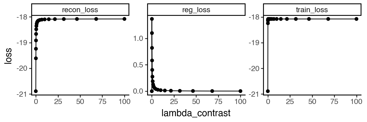
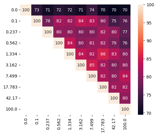
We examined 10 values ranging from 0 to 100 to assess their effect on subspace characteristics (Fig. 10). Our analysis again reveals the clear separation of sPCA solution () from other sisPCA models. As increases, infected cells form a tighter cluster in the infection subspace (Fig. 10a), while temporal dynamics become less pronounced, with increased mixing of cells from different time points (Fig. 10b). Moreover, sisPCA results are quite robust across in preserving subspace structure (Fig. 10c). Since the disentanglement effect primarily manifests in PC2 of the infection subspace, all models, even sPCA, extract similar sets of top contributor genes in PC1 of the infection subspace, thus yielding GO enrichment results comparable to those shown in Fig. 6.


Appendix H Supplementary visualizations of baseline performance in applications.
For completeness, here we provide subspace visualization for baseline models not included in the main figures. Specifically, Fig. 11 shows the full sPCA performance on the simulated data, related to Fig. 3. Fig. 12 visualizes the single-cell subspaces learned by sPCA, VAE, supVAE, and hsVAE-sc, related to Fig. 5.


NeurIPS Paper Checklist
-
1.
Claims
-
Question: Do the main claims made in the abstract and introduction accurately reflect the paper’s contributions and scope?
-
Answer: [Yes]
-
Justification: In the paper, we proposed a multi-subspace extension of PCA to disentangle interpretable subspaces of variations using self-supervision. We believe our work is highly novel and significant to practitioners using PCA as well as general audience in computational biology.
-
Guidelines:
-
•
The answer NA means that the abstract and introduction do not include the claims made in the paper.
-
•
The abstract and/or introduction should clearly state the claims made, including the contributions made in the paper and important assumptions and limitations. A No or NA answer to this question will not be perceived well by the reviewers.
-
•
The claims made should match theoretical and experimental results, and reflect how much the results can be expected to generalize to other settings.
-
•
It is fine to include aspirational goals as motivation as long as it is clear that these goals are not attained by the paper.
-
•
-
2.
Limitations
-
Question: Does the paper discuss the limitations of the work performed by the authors?
-
Answer: [Yes]
-
Justification: See Section 5.
-
Guidelines:
-
•
The answer NA means that the paper has no limitation while the answer No means that the paper has limitations, but those are not discussed in the paper.
-
•
The authors are encouraged to create a separate "Limitations" section in their paper.
-
•
The paper should point out any strong assumptions and how robust the results are to violations of these assumptions (e.g., independence assumptions, noiseless settings, model well-specification, asymptotic approximations only holding locally). The authors should reflect on how these assumptions might be violated in practice and what the implications would be.
-
•
The authors should reflect on the scope of the claims made, e.g., if the approach was only tested on a few datasets or with a few runs. In general, empirical results often depend on implicit assumptions, which should be articulated.
-
•
The authors should reflect on the factors that influence the performance of the approach. For example, a facial recognition algorithm may perform poorly when image resolution is low or images are taken in low lighting. Or a speech-to-text system might not be used reliably to provide closed captions for online lectures because it fails to handle technical jargon.
-
•
The authors should discuss the computational efficiency of the proposed algorithms and how they scale with dataset size.
-
•
If applicable, the authors should discuss possible limitations of their approach to address problems of privacy and fairness.
-
•
While the authors might fear that complete honesty about limitations might be used by reviewers as grounds for rejection, a worse outcome might be that reviewers discover limitations that aren’t acknowledged in the paper. The authors should use their best judgment and recognize that individual actions in favor of transparency play an important role in developing norms that preserve the integrity of the community. Reviewers will be specifically instructed to not penalize honesty concerning limitations.
-
•
-
3.
Theory Assumptions and Proofs
-
Question: For each theoretical result, does the paper provide the full set of assumptions and a complete (and correct) proof?
-
Answer: [Yes]
-
Guidelines:
-
•
The answer NA means that the paper does not include theoretical results.
-
•
All the theorems, formulas, and proofs in the paper should be numbered and cross-referenced.
-
•
All assumptions should be clearly stated or referenced in the statement of any theorems.
-
•
The proofs can either appear in the main paper or the supplemental material, but if they appear in the supplemental material, the authors are encouraged to provide a short proof sketch to provide intuition.
-
•
Inversely, any informal proof provided in the core of the paper should be complemented by formal proofs provided in appendix or supplemental material.
-
•
Theorems and Lemmas that the proof relies upon should be properly referenced.
-
•
-
4.
Experimental Result Reproducibility
-
Question: Does the paper fully disclose all the information needed to reproduce the main experimental results of the paper to the extent that it affects the main claims and/or conclusions of the paper (regardless of whether the code and data are provided or not)?
-
Answer: [Yes]
-
Justification: Details on data preprocessing and model configurations are provided in the corresponding sections and in Appendix F. A Python implementation of sisPCA is available on GitHub (https://github.com/JiayuSuPKU/sispca). The repository also contains notebooks to reproduce most results in the paper main text and in appendices.
-
Guidelines:
-
•
The answer NA means that the paper does not include experiments.
-
•
If the paper includes experiments, a No answer to this question will not be perceived well by the reviewers: Making the paper reproducible is important, regardless of whether the code and data are provided or not.
-
•
If the contribution is a dataset and/or model, the authors should describe the steps taken to make their results reproducible or verifiable.
-
•
Depending on the contribution, reproducibility can be accomplished in various ways. For example, if the contribution is a novel architecture, describing the architecture fully might suffice, or if the contribution is a specific model and empirical evaluation, it may be necessary to either make it possible for others to replicate the model with the same dataset, or provide access to the model. In general. releasing code and data is often one good way to accomplish this, but reproducibility can also be provided via detailed instructions for how to replicate the results, access to a hosted model (e.g., in the case of a large language model), releasing of a model checkpoint, or other means that are appropriate to the research performed.
-
•
While NeurIPS does not require releasing code, the conference does require all submissions to provide some reasonable avenue for reproducibility, which may depend on the nature of the contribution. For example
-
(a)
If the contribution is primarily a new algorithm, the paper should make it clear how to reproduce that algorithm.
-
(b)
If the contribution is primarily a new model architecture, the paper should describe the architecture clearly and fully.
-
(c)
If the contribution is a new model (e.g., a large language model), then there should either be a way to access this model for reproducing the results or a way to reproduce the model (e.g., with an open-source dataset or instructions for how to construct the dataset).
-
(d)
We recognize that reproducibility may be tricky in some cases, in which case authors are welcome to describe the particular way they provide for reproducibility. In the case of closed-source models, it may be that access to the model is limited in some way (e.g., to registered users), but it should be possible for other researchers to have some path to reproducing or verifying the results.
-
(a)
-
•
-
5.
Open access to data and code
-
Question: Does the paper provide open access to the data and code, with sufficient instructions to faithfully reproduce the main experimental results, as described in supplemental material?
-
Answer: [Yes]
-
Justification: We do not generate new data in this study and use public datasets for all analyses. See detailed description on data access and license in the corresponding sections. A Python implementation of sisPCA is available on GitHub (https://github.com/JiayuSuPKU/sispca). The repository also contains notebooks to reproduce most results in the paper main text and in appendices.
-
Guidelines:
-
•
The answer NA means that paper does not include experiments requiring code.
-
•
Please see the NeurIPS code and data submission guidelines (https://nips.cc/public/guides/CodeSubmissionPolicy) for more details.
-
•
While we encourage the release of code and data, we understand that this might not be possible, so “No” is an acceptable answer. Papers cannot be rejected simply for not including code, unless this is central to the contribution (e.g., for a new open-source benchmark).
-
•
The instructions should contain the exact command and environment needed to run to reproduce the results. See the NeurIPS code and data submission guidelines (https://nips.cc/public/guides/CodeSubmissionPolicy) for more details.
-
•
The authors should provide instructions on data access and preparation, including how to access the raw data, preprocessed data, intermediate data, and generated data, etc.
-
•
The authors should provide scripts to reproduce all experimental results for the new proposed method and baselines. If only a subset of experiments are reproducible, they should state which ones are omitted from the script and why.
-
•
At submission time, to preserve anonymity, the authors should release anonymized versions (if applicable).
-
•
Providing as much information as possible in supplemental material (appended to the paper) is recommended, but including URLs to data and code is permitted.
-
•
-
6.
Experimental Setting/Details
-
Question: Does the paper specify all the training and test details (e.g., data splits, hyperparameters, how they were chosen, type of optimizer, etc.) necessary to understand the results?
-
Answer: [Yes]
-
Justification: Details on data preprocessing, model configuration and hyperparameter selection are described in the corresponding sections and in Appendix F.
-
Guidelines:
-
•
The answer NA means that the paper does not include experiments.
-
•
The experimental setting should be presented in the core of the paper to a level of detail that is necessary to appreciate the results and make sense of them.
-
•
The full details can be provided either with the code, in appendix, or as supplemental material.
-
•
-
7.
Experiment Statistical Significance
-
Question: Does the paper report error bars suitably and correctly defined or other appropriate information about the statistical significance of the experiments?
-
Answer: [No]
-
Justification: Statistical significance tests are not included in this paper due to the nature of our experiments, which primarily focus on qualitative performance assessments and biological interpretations lacking quantitative null hypotheses. The quantitative performance evaluations presented in the tables are self-evident and serve to demonstrate design principles. Moreover, our baseline models (PCA and sPCA) are deterministic, eliminating the need for error bars or confidence intervals that typically account for randomness.
-
Guidelines:
-
•
The answer NA means that the paper does not include experiments.
-
•
The authors should answer "Yes" if the results are accompanied by error bars, confidence intervals, or statistical significance tests, at least for the experiments that support the main claims of the paper.
-
•
The factors of variability that the error bars are capturing should be clearly stated (for example, train/test split, initialization, random drawing of some parameter, or overall run with given experimental conditions).
-
•
The method for calculating the error bars should be explained (closed form formula, call to a library function, bootstrap, etc.)
-
•
The assumptions made should be given (e.g., Normally distributed errors).
-
•
It should be clear whether the error bar is the standard deviation or the standard error of the mean.
-
•
It is OK to report 1-sigma error bars, but one should state it. The authors should preferably report a 2-sigma error bar than state that they have a 96% CI, if the hypothesis of Normality of errors is not verified.
-
•
For asymmetric distributions, the authors should be careful not to show in tables or figures symmetric error bars that would yield results that are out of range (e.g. negative error rates).
-
•
If error bars are reported in tables or plots, The authors should explain in the text how they were calculated and reference the corresponding figures or tables in the text.
-
•
-
8.
Experiments Compute Resources
-
Question: For each experiment, does the paper provide sufficient information on the computer resources (type of compute workers, memory, time of execution) needed to reproduce the experiments?
-
Answer: [Yes]
-
Justification: We discuss the computational complexity of sisPCA in Appendix D. The proposed method is highly efficient because of the linearity. We ran all provided notebooks (https://github.com/JiayuSuPKU/sispca/tree/main/docs/source/tutorials) using a personal M1 Macbook Air with 16GB RAM and completed most analysis steps in minutes including model training.
-
Guidelines:
-
•
The answer NA means that the paper does not include experiments.
-
•
The paper should indicate the type of compute workers CPU or GPU, internal cluster, or cloud provider, including relevant memory and storage.
-
•
The paper should provide the amount of compute required for each of the individual experimental runs as well as estimate the total compute.
-
•
The paper should disclose whether the full research project required more compute than the experiments reported in the paper (e.g., preliminary or failed experiments that didn’t make it into the paper).
-
•
-
9.
Code Of Ethics
-
Question: Does the research conducted in the paper conform, in every respect, with the NeurIPS Code of Ethics https://neurips.cc/public/EthicsGuidelines?
-
Answer: [Yes]
-
Justification: We confirm the work conforms with the code of ethics.
-
Guidelines:
-
•
The answer NA means that the authors have not reviewed the NeurIPS Code of Ethics.
-
•
If the authors answer No, they should explain the special circumstances that require a deviation from the Code of Ethics.
-
•
The authors should make sure to preserve anonymity (e.g., if there is a special consideration due to laws or regulations in their jurisdiction).
-
•
-
10.
Broader Impacts
-
Question: Does the paper discuss both potential positive societal impacts and negative societal impacts of the work performed?
-
Answer: [N/A]
-
Justification: This paper presents work whose goal is to advance the field of Machine Learning. There are many potential societal consequences of our work, none which we feel must be specifically highlighted here.
-
Guidelines:
-
•
The answer NA means that there is no societal impact of the work performed.
-
•
If the authors answer NA or No, they should explain why their work has no societal impact or why the paper does not address societal impact.
-
•
Examples of negative societal impacts include potential malicious or unintended uses (e.g., disinformation, generating fake profiles, surveillance), fairness considerations (e.g., deployment of technologies that could make decisions that unfairly impact specific groups), privacy considerations, and security considerations.
-
•
The conference expects that many papers will be foundational research and not tied to particular applications, let alone deployments. However, if there is a direct path to any negative applications, the authors should point it out. For example, it is legitimate to point out that an improvement in the quality of generative models could be used to generate deepfakes for disinformation. On the other hand, it is not needed to point out that a generic algorithm for optimizing neural networks could enable people to train models that generate Deepfakes faster.
-
•
The authors should consider possible harms that could arise when the technology is being used as intended and functioning correctly, harms that could arise when the technology is being used as intended but gives incorrect results, and harms following from (intentional or unintentional) misuse of the technology.
-
•
If there are negative societal impacts, the authors could also discuss possible mitigation strategies (e.g., gated release of models, providing defenses in addition to attacks, mechanisms for monitoring misuse, mechanisms to monitor how a system learns from feedback over time, improving the efficiency and accessibility of ML).
-
•
-
11.
Safeguards
-
Question: Does the paper describe safeguards that have been put in place for responsible release of data or models that have a high risk for misuse (e.g., pretrained language models, image generators, or scraped datasets)?
-
Answer: [N/A]
-
Justification: This paper poses no such risks.
-
Guidelines:
-
•
The answer NA means that the paper poses no such risks.
-
•
Released models that have a high risk for misuse or dual-use should be released with necessary safeguards to allow for controlled use of the model, for example by requiring that users adhere to usage guidelines or restrictions to access the model or implementing safety filters.
-
•
Datasets that have been scraped from the Internet could pose safety risks. The authors should describe how they avoided releasing unsafe images.
-
•
We recognize that providing effective safeguards is challenging, and many papers do not require this, but we encourage authors to take this into account and make a best faith effort.
-
•
-
12.
Licenses for existing assets
-
Question: Are the creators or original owners of assets (e.g., code, data, models), used in the paper, properly credited and are the license and terms of use explicitly mentioned and properly respected?
-
Answer: [Yes]
-
Justification: The Kaggle Breast Cancer Wisconsin Dataset is publicly available under CC BY-NC-SA 4.0. The TCGA methylation dataset has controlled access due to privacy regulation. The single-cell malaria liver infection data is publicly available under CC-BY 4.0.
-
Guidelines:
-
•
The answer NA means that the paper does not use existing assets.
-
•
The authors should cite the original paper that produced the code package or dataset.
-
•
The authors should state which version of the asset is used and, if possible, include a URL.
-
•
The name of the license (e.g., CC-BY 4.0) should be included for each asset.
-
•
For scraped data from a particular source (e.g., website), the copyright and terms of service of that source should be provided.
-
•
If assets are released, the license, copyright information, and terms of use in the package should be provided. For popular datasets, paperswithcode.com/datasets has curated licenses for some datasets. Their licensing guide can help determine the license of a dataset.
-
•
For existing datasets that are re-packaged, both the original license and the license of the derived asset (if it has changed) should be provided.
-
•
If this information is not available online, the authors are encouraged to reach out to the asset’s creators.
-
•
-
13.
New Assets
-
Question: Are new assets introduced in the paper well documented and is the documentation provided alongside the assets?
-
Answer: [N/A]
-
Justification: The paper does not release new assets.
-
Guidelines:
-
•
The answer NA means that the paper does not release new assets.
-
•
Researchers should communicate the details of the dataset/code/model as part of their submissions via structured templates. This includes details about training, license, limitations, etc.
-
•
The paper should discuss whether and how consent was obtained from people whose asset is used.
-
•
At submission time, remember to anonymize your assets (if applicable). You can either create an anonymized URL or include an anonymized zip file.
-
•
-
14.
Crowdsourcing and Research with Human Subjects
-
Question: For crowdsourcing experiments and research with human subjects, does the paper include the full text of instructions given to participants and screenshots, if applicable, as well as details about compensation (if any)?
-
Answer: [N/A]
-
Justification: The paper does not involve crowdsourcing nor research with human subjects.
-
Guidelines:
-
•
The answer NA means that the paper does not involve crowdsourcing nor research with human subjects.
-
•
Including this information in the supplemental material is fine, but if the main contribution of the paper involves human subjects, then as much detail as possible should be included in the main paper.
-
•
According to the NeurIPS Code of Ethics, workers involved in data collection, curation, or other labor should be paid at least the minimum wage in the country of the data collector.
-
•
-
15.
Institutional Review Board (IRB) Approvals or Equivalent for Research with Human Subjects
-
Question: Does the paper describe potential risks incurred by study participants, whether such risks were disclosed to the subjects, and whether Institutional Review Board (IRB) approvals (or an equivalent approval/review based on the requirements of your country or institution) were obtained?
-
Answer: [N/A]
-
Justification: The paper does not involve crowdsourcing nor research with human subjects.
-
Guidelines:
-
•
The answer NA means that the paper does not involve crowdsourcing nor research with human subjects.
-
•
Depending on the country in which research is conducted, IRB approval (or equivalent) may be required for any human subjects research. If you obtained IRB approval, you should clearly state this in the paper.
-
•
We recognize that the procedures for this may vary significantly between institutions and locations, and we expect authors to adhere to the NeurIPS Code of Ethics and the guidelines for their institution.
-
•
For initial submissions, do not include any information that would break anonymity (if applicable), such as the institution conducting the review.
-
•