DisenGCD: A Meta Multigraph-assisted Disentangled Graph Learning Framework for Cognitive Diagnosis

This paper only employs the student-exercise-concept interaction graph $\mathcal{G_{I}}$ for students’ representation learning, and disentangles two graphs from $\mathcal{G_{I}}$ for the remaining two types of representation learning, which are the exercise-concept relation graph $\mathcal{G_{R}}$, and the concept dependency graph $\mathcal{G_{D}}$.

For the cognitive diagnosis task in an intelligent education online platform, there are usually three sets of items: a set of $N$ students $S=\{s_{1},s_{2},\ldots,s_{N}\}$, a set of $M$ exercises $E=\{e_{1},e_{2},\ldots,e_{M}\}$, and a set of $K$ knowledge concepts (concept for short) $C=\{c_{1},c_{2},\ldots,c_{K}\}$. Besides, there commonly exists two matrices: exercise-concept relation matrix $Q=(Q_{jk}\in\{0,1\})^{M\times K}$ (Q-matrix) and concept dependency matrix $D=(Q_{km}\in\{0,1\})^{K\times K}$, to show the relationship of exercises to concepts and concepts to concepts, respectively. $Q_{jk}=1$ denotes the concept $c_{k}$ is not included in the exercise $e_{j}$ and $Q_{jk}=0$ otherwise; similarly, $D_{km}=1$ denotes concept $c_{k}$ relies on concept $c_{m}$ and $D_{km}=0$ otherwise. All students’ exercising reponse logs are denoted by $\mathcal{R}=\{(s_{i},e_{j},r_{ij})|s_{i}\in S,e_{j}\in E,r_{ij}\in\{0,1\}\}$, where $r_{ij}$ refers to the response/answer of student $s_{i}$ on exercise $e_{j}$. $r_{ij}=1$ means the answer is correct and $r_{ij}=0$ otherwise.

The CD based on disentangled graphs is defined as follows: Given: students’ response logs $\mathcal{R}$ and three disentangled graphs: interaction graph $\mathcal{G_{I}}$, relation graph $\mathcal{G_{R}}$, and dependency graph $\mathcal{G_{D}}$; Goal: revealing students’ proficiency on concepts by predicting students’ responses through NNs.

Based on interaction graph $\mathcal{G_{I}}$, this module is responsible for: learning the optimal meta multigraph structure in $\mathcal{G_{I}}$, i.e., optimal multiple propagation paths, and updating student nodes’ representations based on the learned meta multigraph structure to get the representation $\overline{\mathbf{S_{i}}}\in\mathbb{R}^{1\times d}$.

To start with, all nodes (including students, exercises, and concepts) need to be mapped into a $d$-dimensional hidden space. The student embedding $\mathbf{s}_{i}\in\mathbb{R}^{1\times d}$ for student $s_{i}$, exercise embedding $\mathbf{e}_{j}^{I}\in\mathbb{R}^{1\times d}$ for exercise $e_{j}$, and concept embedding $\mathbf{c}_{k}^{I}\in\mathbb{R}^{1\times d}$ for concept $c_{k}$ can be obtained by

$\mathbf{x}_{i}^{S}\in\{0,1\}^{1\times N}$, $\mathbf{x}_{j}^{E}\in\{0,1\}^{1\times M}$, and $\mathbf{x}_{k}^{C}\in\{0,1\}^{1\times K}$ are three one-hot vectors for student $s_{i}$, exercise $e_{j}$, concept $c_{k}$, respecitvely. $W_{S}^{I}$, $W_{E}^{I}$, and $W_{C}^{I}$ are three learnable parameter matrices.

GAT-based Exercise Learning Module. This module is responsible for learning the exercise representation $\overline{\mathbf{E_{j}}}\in\mathbb{R}^{1\times d}$ on the relation graph $\mathcal{G_{R}}$ via a $L$-layer GAT network [24]. Firstly, the embedding of exercises and concepts in $\mathcal{G_{R}}$ is obtained in the manner same as Eq.(1) through two learnable matrices $W_{E}^{R}\in\mathbb{R}^{M\times d}$ and $W_{C}^{R}\in\mathbb{R}^{K\times d}$, i.e, $\mathbf{e}_{j}^{R}=\mathbf{x}_{j}^{E}\times W_{E}^{R},\mathbf{c}_{k}^{R}=\mathbf{x}_{k}^{C}\times W_{C}^{R}$.

Afterward, the GAT neural network is applied to aggregate neighbor information to learn the exercise representation. The aggregation process of $l$-th layer ($1\leq l\leq L$) can be represented as

The first equation is to aggregate the information of exercise $e_{j}$’s neighbors $N_{e_{j}}$ to get its $l$-th layer’s latent representation $\mathbf{e}_{j}^{R(l)}\in\mathbb{R}^{1\times d}$, while the second is to update the $l$-th layer’s concept latent representation $\mathbf{c}_{k}^{R(l)}\in\mathbb{R}^{1\times d}$ from its exercise neighbors $N_{c_{k}}^{ec}$ and concept neighbors $N_{c_{k}}^{cc}$. $\alpha_{j}^{R(l)}$, $\alpha_{k}^{R(l)}$, and $\alpha_{\hat{k}}^{R(l)}$ are the $l$-th layer’s attention matrices for exercise $e_{j}$’s concept neighbors, concept $c_{k}$’s exercise neighbors, and $c_{k}$’s concept neighbors. They can be obtained in the same manner, and the $k$-th row of $\alpha_{j}^{R(l)}$ can be obtained by

$[\cdot]$ is the concatenation and $F_{ec}(\cdot)$ is a fully connected (FC) layer mapping $2*d$ vectors to scalars.

The latent representation $\mathbf{e}_{j}^{R(0)}$ and $\mathbf{c}_{k}^{R(0)}$ refer to $\mathbf{e}_{j}^{R}$ and $\mathbf{c}_{k}^{R}$, and the $L$-th layer output $\mathbf{e}_{j}^{R(L)}$ is used as $\overline{\mathbf{E}_{j}}$. By disentangling the interaction data, the learned exercise representation $\overline{\mathbf{E}_{j}}$ will be more robust against interaction noise.

GAT-based Concept Learning Module. Similarly, this module obtains the concept representation $\overline{\mathbf{C}_{k}}\in\mathbb{R}^{1\times d}$ by applying a $L$-layer GAT network to the dependency graph $\mathcal{G_{D}}$. After obtaining the initial embedding $\mathbf{c}_{k}^{D}=\mathbf{x}_{k}^{C}\times W_{C}^{D}$ by a learnable matrix $W_{C}^{D}\in\mathbb{R}^{K\times d}$, this module updates the $l$-th layer’s latent representation $\mathbf{c}_{k}^{D(l)}$ by $\mathbf{c}_{k}^{D(l)}=\textstyle\sum_{m\in N_{c_{k}}^{cc}}\alpha_{\hat{k}(m)}^{D(l)}\mathbf{c}_{m}^{D(l-1)}+\mathbf{c}_{k}^{D(l-1)}$. $\alpha_{\hat{k}}^{D(l)}$ denotes the attention matrix, which can be computed as same as Eq.(7).

Here $\mathbf{c}_{k}^{D(0)}$ is equal to $\mathbf{c}_{k}^{D}$, and the $L$-th layer output $\mathbf{c}_{k}^{D(L)}$ is used as $\overline{\mathbf{C}_{k}}$. If graph $\mathcal{G_{D}}$ is unavailable, this module will directly take the initial embedding $\mathbf{c}_{k}^{D}$ as $\overline{\mathbf{C}_{k}}$. By further disentangling, the learned representation $\overline{\mathbf{C}_{k}}$ may be robust against noise in student interactions to some extent.

To effectively handle the obtained three types of representations, a novel diagnostic function is proposed to predict the response $\hat{r_{ij}}$ of student $s_{i}$ got on exercise $e_{j}$ as follows:

where $F_{si}(\cdot)$, $F_{ej}(\cdot)$, and $F_{simi}(\cdot)$ are three FC layers mapping a $d$-dimensional vector to another one, and $Q_{k}$ is a binary vector in the $k$-th row of Q-matrix.

Here $\mathbf{h}_{si}\in\mathbb{R}^{1\times d}$ can be seen as the student’s mastery of each knowledge concept; while the obtaining of $\mathbf{h}_{ej}\in\mathbb{R}^{1\times d}$ aims to get the exercise difficulty of each concept; $\mathbf{h}_{simi}$ is to measure the similarity between $\mathbf{h}_{si}$ and $\mathbf{h}_{ej}$ via a dot-product followed by an FC layer and a Sigmoid function $\sigma(\cdot)$ [41], where a higher similarity value in each bit represents a higher mastery on each concept, further indicating a higher probability of answering the related exercises; the last equation follows the idea of NCD to compute the overall mastery averaged over all concepts contained in exercise $e_{j}$.

We can see that the proposed diagnostic function has as high interpretability as NCD, IRT, and MIRT.

Model Optimization. With the above modules, the proposed DisenGCD are trained by solving the following bilevel optimization problem through Adam [39]:

where $\mathcal{L}_{val}(\cdot)$ and $\mathcal{L}_{train}(\cdot)$ denote the loss on validation dataset $D_{val}$ and training dataset $D_{train}$. $\boldsymbol{\omega}$ denotes all model parameters, and $\boldsymbol{\alpha}$ denotes the weights of learnable propagation paths $\mathcal{AP}$ in meta multigraph $MG$. The cross-entropy loss [40] is used for $\mathcal{L}_{val}$ and $\mathcal{L}_{train}$.

Datasets. To verify the DisenGCD’s effectiveness, we conducted experiments on two public datasets ASSISTments [6] and SLP [14], and one private dataset Math, whose statistics are in Table 1. Note that ASSISTments and Math [16] were used for most experiments to answer RQ1 to RQ3, and SLP was used to answer RQ4. More details of these datasets are presented in Appendix A.2.

To address RQ1, the DisenGCD was compared with DINA, MIRT, NCD, ECD, and RCD on ASSISTments and Math datasets. Table 2 summarizes their performance in terms of AUC, ACC, and RMSE obtained under four dataset-splitting settings, where the best result of each column on one dataset was highlighted in bold. Besides, Table 6 in the Appendix compares DisenGCD with three SOTA CDMs, including SCD [28], KSCD [15], and KaNCD [26].

We can observe from the results in both tables that, DisenGCD holds better performance than all compared CDMs. Besides, we can also obtain two observations from Table 2: Firstly, GNN-based CDMs (RCD and DisenGCD) hold significantly better than NN-based CDMs (NCD and ECD), indicating the importance of learning representations through graphs, and DisenGCD outperforming RCD validates the superiority of DisenGCD’s graph learning manner. Secondly, as the ratio changes, the performance change of DisenGCD and RCD is much smaller than NCD and ECD, which signifies DisenGCD and RCD are more robust to different-sparsity data. To validate its sparsity superiority, more experiments are summarized in Appendix B.1.

To investigate DisenGCD’s robustness against interaction noise, we conducted robust experiments on the ASSISTments dataset under the ratio of 60%/10%/30%, where a certain amount of noise interactions were added to each student in the training and validation datasets. Figure 3a presents the ACC and AUC of DisenGCD and RCD under noise data of different percentages. As the noise data increases, the performance leading of DisenGCD over RCD becomes more significant, which reaches maximal when noise data of 50% was added. That demonstrates DisenGCD is more robust to student noise interactions than RCD, attributed to the disentangled learning framework of DisenGCD. Similar observations can be drawn from more experiments on other two datasets in Appendix B.2.

To further analyze the framework effectiveness, four variants of DisenGCD were created: DisenGCD(I) refers to learning three representations only on the interaction graph $\mathcal{G_{I}}$; DisenGCD(Is+Rec) refers to learning student representation on $\mathcal{G_{I}}$, but learning exercise and concept ones on the relation graph $\mathcal{G_{R}}$; DisenGCD(Ise+Rc) refers to learning student and exercise representations on $\mathcal{G_{I}}$ but learning concept one on $\mathcal{G_{R}}$; while DisenGCD(Isc+Re) learns student and concept representations on $\mathcal{G_{I}}$ but learns exercise one on $\mathcal{G_{R}}$. Table 3 compares the performance of RCD, DisenGCD, and its four variants on ASSISTments. As can be seen, the comparison between DisenGCD(I) and other variants indicates learning three representations in two disentangled graphs is more effective than in one unified graph, especially with textitDisenGCD(Is+Rec); the comparison between DisenGCD(Is+Rec) and DisenGCD indicates learning three representations in three disentangled graphs is more effective, further validating the above conclusion. Finally, we can conclude that the proposed disentangled learning framework is effective in enhancing DisenGCD’s performance and robustness.

In Table 3, both DisenGCD(I) and RCD learn three types of representations in one unified graph, but DisenGCD(I) utilizes the meta multigraph aggregator. Therefore, the comparison between DisenGCD(I) and RCD proves the devised meta multigraph learning module is effective in improving the model performance to some extent.

To further validate this, we created three variants of DisenGCD: DisenGCD(naive) refers to the meta multigraph module replaced by the naive embedding (i.e., $\overline{\mathbf{S_{i}}}$ equal to $\mathbf{s}_{i}$ in Eq.(1)); DisenGCD(mp) refers to predefining the meta multigraph module’s propagation paths according to HAN [30]; DisenGCD(mg) refers to this module’s meta multigraph replaced by meta graph. Figure 3b presents the AUC and ACC values of DisenGDCN and its variants on two datasets under the ratio of 60%/10%/30%. As can be seen, the devised meta multigraph learning module enables DisenGDCN to hold significantly better performance than the naive embedding-based variant. The comparison results between DisenGCD and DisenGCD(mg) as well as DisenGCD(mp) validates the effectiveness of using meta multigraph and the automatically learned propagation paths (i.e., learned meta multigraph). Thus, the effectiveness of the devised meta multigraph module can be validated.

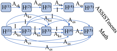
The comparison between DisenGCD(mp) and DisenGCD has revealed the effectiveness of the learned meta multigraph on the target dataset. Therefore, an intuitive doubt naturally emerged: Is the learned meta multigraph still effective on other datasets? Before solving this, Figure 4a gives the structure visualization of two learned meta multigraphs. We can see two learned meta multigraphs hold two distinct structures. That may be because two datasets are a bit different regarding the relations between exercises and concepts, where exercises in Math contain only one concept while exercises in ASSISTments may contain more than one concept. Thus, another doubt naturally emerged: Is the learned meta multigraph on the target dataset ineffective on a different type of dataset?

To solve the doubts, we applied six learned meta multigraphs (A1, A2, A3, M1, M2, and M3) to the SLP. A1-A3 and M1-M3 were learned by DisenGCD three times on ASSISTments and Math. SLP dataset is similar to Math, whose exercises only contain one concept. Figure 4b summarizes the results of RCD and six DisenGCD variants that utilize six given meta multigraphs. As can be seen, DisenGCD’s performance under M1-M3 is promising and better than RCD, while DisenGCD under A1-A3 performed poorly. The observation can answer the above doubts to some extent: meta multigraphs learned by DisenGCD may be effective when the datasets to be applied are similar to target datasets.

In addition to the above four experiments, more experiments were executed to validate the devised diagnostic functions, analyze the DisenGCD’s parameter sensitivity, analyze its execution efficiency, and investigate the effectiveness of the employed GAT modules in Appendix B.3, Appendix B.4, Appendix B.5, and Appendix B.6.

References

- [1] Ashton Anderson, Daniel Huttenlocher, Jon Kleinberg, and Jure Leskovec. Engaging with massive online courses. In Proceedings of the 23rd international conference on World wide web, pages 687–698, 2014.
- [2] Joseph Beck. Difficulties in inferring student knowledge from observations (and why you should care). In Proceedings of the 13th International Conference of Artificial Intelligence in Education, pages 21–30, 2007.
- [3] Song Cheng, Qi Liu, Enhong Chen, Zai Huang, Zhenya Huang, Yiying Chen, Haiping Ma, and Guoping Hu. Dirt: Deep learning enhanced item response theory for cognitive diagnosis. In Proceedings of the 28th ACM international conference on information and knowledge management, pages 2397–2400, 2019.
- [4] Jimmy De La Torre. Dina model and parameter estimation: A didactic. Journal of educational and behavioral statistics, 34(1):115–130, 2009.
- [5] Yuhui Ding, Quanming Yao, Huan Zhao, and Tong Zhang. Diffmg: Differentiable meta graph search for heterogeneous graph neural networks. In Proceedings of the 27th ACM SIGKDD Conference on Knowledge Discovery & Data Mining, pages 279–288, 2021.
- [6] Mingyu Feng, Neil Heffernan, and Kenneth Koedinger. Addressing the assessment challenge with an online system that tutors as it assesses. User Modeling and User-adapted Interaction, 19(3):243–266, 2009.
- [7] Weibo Gao, Qi Liu, Zhenya Huang, Yu Yin, Haoyang Bi, Mu-Chun Wang, Jianhui Ma, Shijin Wang, and Yu Su. Rcd: Relation map driven cognitive diagnosis for intelligent education systems. In Proceedings of the 44th international ACM SIGIR conference on research and development in information retrieval, pages 501–510, 2021.
- [8] Zhenyu Han, Fengli Xu, Jinghan Shi, Yu Shang, Haorui Ma, Pan Hui, and Yong Li. Genetic meta-structure search for recommendation on heterogeneous information network. In Proceedings of the 29th ACM International Conference on Information & Knowledge Management, pages 455–464, 2020.
- [9] Xiangnan He, Kuan Deng, Xiang Wang, Yan Li, YongDong Zhang, and Meng Wang. Lightgcn: Simplifying and powering graph convolution network for recommendation. In Proceedings of the 43rd International ACM SIGIR Conference on Research and Development in Information Retrieval, SIGIR ’20, page 639–648, New York, NY, USA, 2020. Association for Computing Machinery.
- [10] Chao Li, Hao Xu, and Kun He. Differentiable meta multigraph search with partial message propagation on heterogeneous information networks. In Proceedings of the AAAI Conference on Artificial Intelligence, volume 37, pages 8518–8526, 2023.
- [11] Qi Liu, Shiwei Tong, Chuanren Liu, Hongke Zhao, Enhong Chen, Haiping Ma, and Shijin Wang. Exploiting cognitive structure for adaptive learning. In Proceedings of the 25th ACM SIGKDD International Conference on Knowledge Discovery & Data Mining, pages 627–635, 2019.
- [12] Sannyuya Liu, Qing Li, Xiaoxuan Shen, Jianwen Sun, and Zongkai Yang. Automated discovery of symbolic laws governing skill acquisition from naturally occurring data. Nature Computational Science, pages 1–12, 2024.
- [13] Frederique M Lord. Applications of Item Response Theory to Practical Testing Problems. LAWRENCE ERLBAUM ASSCCIAATES, 1980.
- [14] Yu Lu, Yang Pian, Ziding Shen, Penghe Chen, and Xiaoqing Li. SLP: A multi-dimensional and consecutive dataset from K-12 education. In Proceedings of the 29th International Conference on Computers in Education Conference, volume 1, pages 261–266. Asia-Pacific Society for Computers in Education, 2021.
- [15] Haiping Ma, Manwei Li, Le Wu, Haifeng Zhang, Yunbo Cao, Xingyi Zhang, and Xuemin Zhao. Knowledge-sensed cognitive diagnosis for intelligent education platforms. In Proceedings of the 31st ACM International Conference on Information & Knowledge Management, pages 1451–1460, 2022.
- [16] Haiping Ma, Changqian Wang, Hengshu Zhu, Shangshang Yang, Xiaoming Zhang, and Xingyi Zhang. Enhancing cognitive diagnosis using un-interacted exercises: A collaboration-aware mixed sampling approach. In Proceedings of the AAAI Conference on Artificial Intelligence, volume 38, pages 8877–8885, 2024.
- [17] Haiping Ma, Yong Yang, Chuan Qin, Xiaoshan Yu, Shangshang Yang, Xingyi Zhang, and Hengshu Zhu. Hd-kt: Advancing robust knowledge tracing via anomalous learning interaction detection. In Proceedings of the ACM on Web Conference 2024, pages 4479–4488, 2024.
- [18] Haiping Ma, Yi Zeng, Shangshang Yang, Chuan Qin, Xingyi Zhang, and Limiao Zhang. A novel computerized adaptive testing framework with decoupled learning selector. Complex & Intelligent Systems, pages 1–12, 2023.
- [19] Jianxin Ma, Peng Cui, Kun Kuang, Xin Wang, and Wenwu Zhu. Disentangled graph convolutional networks. In International Conference on Machine Learning, 2019.
- [20] Mark D. Reckase. Multidimensional Item Response Theory. Springer New York, 2009.
- [21] Yu Su, Zeyu Cheng, Jinze Wu, Yanmin Dong, Zhenya Huang, Le Wu, Enhong Chen, Shijin Wang, and Fei Xie. Graph-based cognitive diagnosis for intelligent tutoring systems. Knowledge-Based Systems, 253:109547, 2022.
- [22] Jianwen Sun, Fenghua Yu, Sannyuya Liu, Yawei Luo, Ruxia Liang, and Xiaoxuan Shen. Adversarial bootstrapped question representation learning for knowledge tracing. In Proceedings of the 31st ACM International Conference on Multimedia, pages 8016–8025, 2023.
- [23] Jianwen Sun, Fenghua Yu, Qian Wan, Qing Li, Sannyuya Liu, and Xiaoxuan Shen. Interpretable knowledge tracing with multiscale state representation. In Proceedings of the ACM on Web Conference 2024, pages 3265–3276, 2024.
- [24] Petar Veličković, Guillem Cucurull, Arantxa Casanova, Adriana Romero, Pietro Lio, and Yoshua Bengio. Graph attention networks. arXiv preprint arXiv:1710.10903, 2017.
- [25] Fei Wang, Qi Liu, Enhong Chen, Zhenya Huang, Yuying Chen, Yu Yin, Zai Huang, and Shijin Wang. Neural cognitive diagnosis for intelligent education systems. In Proceedings of the AAAI conference on artificial intelligence, volume 34, pages 6153–6161, 2020.
- [26] Fei Wang, Qi Liu, Enhong Chen, Zhenya Huang, Yu Yin, Shijin Wang, and Yu Su. Neuralcd: a general framework for cognitive diagnosis. IEEE Transactions on Knowledge and Data Engineering, 35(8):8312–8327, 2022.
- [27] Hao Wang, Tong Xu, Qi Liu, Defu Lian, Enhong Chen, Dongfang Du, Han Wu, and Wen Su. Mcne: An end-to-end framework for learning multiple conditional network representations of social network. In Proceedings of the 25th ACM SIGKDD international conference on knowledge discovery & data mining, pages 1064–1072, 2019.
- [28] Shanshan Wang, Zhen Zeng, Xun Yang, and Xingyi Zhang. Self-supervised graph learning for long-tailed cognitive diagnosis. In Proceedings of the AAAI Conference on Artificial Intelligence, volume 37, pages 110–118, 2023.
- [29] Xiang Wang, Hongye Jin, An Zhang, Xiangnan He, Tong Xu, and Tat-Seng Chua. Disentangled graph collaborative filtering. Proceedings of the 43rd International ACM SIGIR Conference on Research and Development in Information Retrieval, 2020.
- [30] Xiao Wang, Houye Ji, Chuan Shi, Bai Wang, Yanfang Ye, Peng Cui, and Philip S Yu. Heterogeneous graph attention network. In The world wide web conference, pages 2022–2032, 2019.
- [31] Xinping Wang, Caidie Huang, Jinfang Cai, and Liangyu Chen. Using knowledge concept aggregation towards accurate cognitive diagnosis. In Proceedings of the 30th ACM International Conference on Information & Knowledge Management, pages 2010–2019, 2021.
- [32] Yifan Wang, Suyao Tang, Yuntong Lei, Weiping Song, Sheng Wang, and Ming Zhang. Disenhan: Disentangled heterogeneous graph attention network for recommendation. Proceedings of the 29th ACM International Conference on Information & Knowledge Management, 2020.
- [33] Jiahao Wu, Wenqi Fan, Jingfan Chen, Shengcai Liu, Qing Li, and Ke Tang. Disentangled contrastive learning for social recommendation. New York, NY, USA, 2022. Association for Computing Machinery.
- [34] Zhengyang Wu, Ming Li, Yong Tang, and Qingyu Liang. Exercise recommendation based on knowledge concept prediction. Knowledge-Based Systems, 210:106481, 2020.
- [35] Jiashu Zhao Dawei Yin Xubin Ren, Lianghao Xia and Chao Huang. Disentangled contrastive collaborative filtering. In Proceedings of the 46th International ACM SIGIR Conference on Research and Development in Information Retrieval, 2023.
- [36] Shangshang Yang, Haiping Ma, Ying Bi, Ye Tian, Limiao Zhang, Yaochu Jin, and Xingyi Zhang. An evolutionary multi-objective neural architecture search approach to advancing cognitive diagnosis in intelligent education. IEEE Transactions on Evolutionary Computation, 2024.
- [37] Shangshang Yang, Haiping Ma, Cheng Zhen, Ye Tian, Limiao Zhang, Yaochu Jin, and Xingyi Zhang. Designing novel cognitive diagnosis models via evolutionary multi-objective neural architecture search. arXiv preprint arXiv:2307.04429, 2023.
- [38] Shangshang Yang, Linrui Qin, and Xiaoshan Yu. Endowing interpretability for neural cognitive diagnosis by efficient kolmogorov-arnold networks. arXiv preprint arXiv:2405.14399, 2024.
- [39] Shangshang Yang, Xiangkun Sun, Ke Xu, Yuanchao Liu, Ye Tian, and Xingyi Zhang. Hybrid architecture-based evolutionary robust neural architecture search. IEEE Transactions on Emerging Topics in Computational Intelligence, 2024.
- [40] Shangshang Yang, Ye Tian, Cheng He, Xingyi Zhang, Kay Chen Tan, and Yaochu Jin. A gradient-guided evolutionary approach to training deep neural networks. IEEE Transactions on Neural Networks and Learning Systems, 33(9):4861–4875, 2021.
- [41] Shangshang Yang, Ye Tian, Xiaoshu Xiang, Shichen Peng, and Xingyi Zhang. Accelerating evolutionary neural architecture search via multifidelity evaluation. IEEE Transactions on Cognitive and Developmental Systems, 14(4):1778–1792, 2022.
- [42] Shangshang Yang, Haoyu Wei, Haiping Ma, Ye Tian, Xingyi Zhang, Yunbo Cao, and Yaochu Jin. Cognitive diagnosis-based personalized exercise group assembly via a multi-objective evolutionary algorithm. IEEE Transactions on Emerging Topics in Computational Intelligence, 2023.
- [43] Shangshang Yang, Xiaoshan Yu, Ye Tian, Xueming Yan, Haiping Ma, and Xingyi Zhang. Evolutionary neural architecture search for transformer in knowledge tracing. In Thirty-seventh Conference on Neural Information Processing Systems, 2023.
- [44] Shangshang Yang, Cheng Zhen, Ye Tian, Haiping Ma, Yuanchao Liu, Panpan Zhang, and Xingyi Zhang. Evolutionary multi-objective neural architecture search for generalized cognitive diagnosis models. In 2023 5th International Conference on Data-driven Optimization of Complex Systems (DOCS), pages 1–10. IEEE, 2023.
- [45] Mingjia Yin, Hao Wang, Wei Guo, Yong Liu, Suojuan Zhang, Sirui Zhao, Defu Lian, and Enhong Chen. Dataset regeneration for sequential recommendation. In Proceedings of the 30th ACM SIGKDD Conference on Knowledge Discovery and Data Mining, pages 3954–3965, 2024.
- [46] Mingjia Yin, Chuhan Wu, Yufei Wang, Hao Wang, Wei Guo, Yasheng Wang, Yong Liu, Ruiming Tang, Defu Lian, and Enhong Chen. Entropy law: The story behind data compression and llm performance. arXiv preprint arXiv:2407.06645, 2024.
- [47] Xiaoshan Yu, Chuan Qin, Dazhong Shen, Shangshang Yang, Haiping Ma, Hengshu Zhu, and Xingyi Zhang. Rigl: A unified reciprocal approach for tracing the independent and group learning processes. In Proceedings of the 30th ACM SIGKDD Conference on Knowledge Discovery and Data Mining, pages 4047–4058, 2024.
- [48] Yuqiang Zhou, Qi Liu, Jinze Wu, Fei Wang, Zhenya Huang, Wei Tong, Hui Xiong, Enhong Chen, and Jianhui Ma. Modeling context-aware features for cognitive diagnosis in student learning. In Proceedings of the 27th ACM SIGKDD Conference on Knowledge Discovery & Data Mining, pages 2420–2428, 2021.
Appendix A More details about Proposed Method and Datasets
A.1 Notations Summary
For convenient reading and understanding, we have summarized all the notations discussed in the paper in the following two tables. Table 4 summarizes all the notations in the three disentangled graphs, while Table 5 describes the notations of the meta multigraph.