Discrete-time Contraction-based Control of Nonlinear Systems with Parametric Uncertainties using Neural Networks
Abstract
In response to the continuously changing feedstock supply and market demand for products with different specifications, the processes need to be operated at time-varying operating conditions and targets (e.g., setpoints) to improve the process economy, in contrast to traditional process operations around predetermined equilibriums. In this paper, a contraction theory-based control approach using neural networks is developed for nonlinear chemical processes to achieve time-varying reference tracking. This approach leverages the universal approximation characteristics of neural networks with discrete-time contraction analysis and control. It involves training a neural network to learn a contraction metric and differential feedback gain, that is embedded in a contraction-based controller. A second, separate neural network is also incorporated into the control-loop to perform online learning of uncertain system model parameters. The resulting control scheme is capable of achieving efficient offset-free tracking of time-varying references, with a full range of model uncertainty, without the need for controller structure redesign as the reference changes. This is a robust approach that can deal with bounded parametric uncertainties in the process model, which are commonly encountered in industrial (chemical) processes. This approach also ensures the process stability during online simultaneous learning and control. Simulation examples are provided to illustrate the above approach.
Index Terms:
Nonlinear control; neural networks; contraction theory; uncertain nonlinear systems; discrete-time control contraction metricI Introduction
The process industry has seen increasing variability in market demand, with time varying specifications and quantity of products. As an example, there is a trend for produce-to-order operations in polymer [1] and fine chemicals sectors. Variations are also evident in the specifications, costs and supply volume of “raw” materials and energy. Consequently, businesses in the process industry are required to have the flexibility to dynamically adjust the volume and specifications of products, and deal with diverse sources of raw materials to remain competitive [2]. Traditionally, a chemical plant is designed and operated at a certain steady-state operating condition where the plant economy is optimized. The process industry is shifting from the traditional mass production to more agile, cost-effective and dynamic process operation closer to the market, which is the main driver for next-generation “smart plants”. As such, the control systems for modern chemical processes need to have the flexibility to drive a process to any required time-varying operational target (setpoint) to meet the dynamic market demand, with a stability guarantee, especially during the start-up or shut-down of processes.
As most chemical processes are inherently nonlinear, flexible process operation warrants nonlinear control as the target operating conditions may need to vary significantly to minimize the economic cost. Control of nonlinear systems to track a time-varying reference profile and ensure stability (convergence) can be challenging [3]. For general nonlinear systems (e.g., many of them appearing in chemical process systems), common nonlinear control approaches involve stabilization of nonlinear systems with respect to a given fixed equilibrium point, e.g., designing a control Lyapunov function for a given equilibrium point, and based on which, constructing a stabilizing control law. Therefore, every time the reference is changed, a new control Lyapunov function needs to be constructed and the control algorithm needs to be redesigned. This inherent lack of flexibility makes control Lyapunov function-based approaches infeasible for tracking arbitrary time-varying references (such as time-varying product specifications required by the market). To address the above challenge, contraction theory [4, 3] was adopted to study the stability around (or contraction to) arbitrary references and design tracking controllers based on differential dynamics for time-varying (feasible) references of nonlinear systems with stability guarantees and without structural redesign (e.g., [5, 6]).
Neural networks have been used for nonlinear process modeling (e.g.,[7]) due to their ability to universally approximate arbitrary functions, adaptive control [8, 9], finding utilization in model-based control designs, such as model predictive control (MPC) (see, e.g., [10]). Neural networks have also been effectively used in learning control and adaptive control applications [11]. A wide variety of neural network structures are available (e.g., Siamese networks [12]), of which can greatly impact the performance of the trained neural network. However, stability design for neural network-based control is still an open problem. In particular, there are very few results on setpoint-independent nonlinear control, especially when considering (embedding) the neural network within the closed-loop control system. This poses a significant obstacle for the neural network-based control approaches for chemical processes, which are mission critical. It is often impractical to operate a process in a large range of random operating conditions (with sufficient excitations) to produce process data to train neural networks to learn system dynamics (or even directly learn control laws). While such an exploration exercise is often performed for mechanical systems, it is generally infeasible for chemical processes, as many operating conditions may lead to poor product quality and/or inefficient material and energy usage with significant financial penalties. If process stability is not ensured, random process operating conditions can even cause severe safety risks (fires or explosions). Furthermore, chemical processes are typically designed based on known mechanisms and thus chemical process models are often available, although often with model uncertainties such as uncertain parameters within a known range (see, e.g., [13]). As such, one promising approach in chemical process control [14] is to train neural network-based controllers using process data (input/output trajectories) generated from process models and further refine such neural networks using real-world process operating data. An important issue is “safe exploration” (during online simultaneous learning and control using neural networks), i.e., how can the controller explore system trajectories to obtain new operating data, such that the stimulus is sufficient for online learning and refinement of such networks, yet simultaneously ensure process stability by exploiting known trajectories, during online simultaneous learning and control using neural networks. Inspired by [14, 15], we aim to develop such a “safe” neural network-based online learning approach to determine uncertain system parameters by “exploiting” a neural network embedded controller that is designed offline via the contraction theory framework.
To address the problem of controlling discrete-time nonlinear systems with parametric uncertainties, this article presents a systematic approach to obtaining a novel contraction-based controller with online parameter learning that embeds neural networks. Using properties of contracting discrete-time systems, we develop a novel approach that uses neural networks to synthesize DCCMs. This approach utilizes the nonlinear process model to train the DCCM neural network representations of the DCCM and differential feedback control gain (from which the control law can be computed). To train the DCCM neural network, a Siamese (or twin) neural network [12] is employed to ensure both steps in the state trajectory share the same state-dependent DCCM. A neural network-based learning module is also incorporated into the control-loop, such that any uncertain parameters can be identified online. Finally, conditions to ensure offset-free tracking (after system parameters are correctly identified), or bounded tracking (when parameters are modeled with known uncertainty bounds), to feasible references are derived. The resulting contraction-based controller embeds a neural network.
This article is structured as follows. Section II formulates the problem of tracking-time varying references for uncertain nonlinear systems with neural networks in the closed loop, and the proposed approach which leverages the contraction theory framework. Section III presents the main approach to designing a discrete-time contraction-based controller for discrete-time systems with parametric uncertainties using DCCM neural networks and learning of uncertain parameters via estimation neural networks. Section IV develops the conditions for the existence of contracting regions under the proposed neural network-based method of Section III. Section V presents illustrative examples, followed by Section VI which concludes the article.
Notation.
Function is defined as for any function , represents the set of all integers, represents the set of positive integers, represents set of real numbers.
II Problem Formulation and Approach
II-A Contraction Theory Overview
Contraction theory [4, 3] facilitates stability analysis and control of discrete-time nonlinear systems with respect to arbitrary, time-varying (feasible) references, without redesigning the control algorithm, through the study of corresponding displacement dynamics or differential dynamics. The analysis and controller synthesis to ensure stability/contraction of the nonlinear system is simultaneously completed via discrete-time control contraction metrics (DCCMs). To introduce the contraction-based methodology, we firstly consider the discrete-time nonlinear control affine system without uncertainty (extended in later sections)
| (1) |
where state and control are and . The corresponding differential system of (1) is as follows
| (2) |
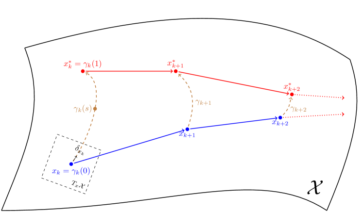
where Jacobian matrices of and in (1) are defined as and respectively, and are vectors in the tangent space at and at respectively, where parameterises a path, between two points such that (see Fig. 1). Considering a state-feedback control law for the differential dynamics (2),
| (3) |
where is a state dependent function, we then have from [4, 3] the following definition for a contracting system.
Definition 1.
A region of state space is called a contraction region if condition (4) holds for all points in that region. In Definition 1, is a metric used in describing the geometry of Riemannian space, which we briefly present here. We define the Riemannian distance, , as a measure for the tracking performance (convergence/stability of the state, , to the reference, ), and is defined as (see, e.g., [16])
| (5) |
where . The shortest path in Riemannian space, or geodesic, between and is defined as
| (6) |
Leveraging Riemannian tools, one feasible feedback tracking controller for (1), can be obtained by integrating the differential feedback law (3) along the geodesic, (6), as
| (7) |
Note, that this particular formulation is reference-independent, since the target trajectory variations do not require structural redesign of the feedback controller and is naturally befitting to the flexible manufacturing paradigm. Moreover, the discrete-time control input, (7), is a function with arguments (, , ) and hence the control action is computed from the current state and target trajectory.
Then, under Definition 1 for a contracting system, e.g., (1) driven by (7), we have
| (8) |
which states that the Riemannian distance between the state trajectory, , and a desired trajectory, is shrinking (i.e., convergence of the state to the reference), with respect to the DCCM, , with at least constant rate.
II-B System Description
To address parametric uncertainties, for the remainder of this article, we consider the following discrete-time control affine nonlinear system with parametric uncertainty
| (9) |
where vector represents the bounded uncertain parameters,
| (10) |
and functions and are smooth along the direction and Lipschitz continuous along . The corresponding differential dynamics (and hence the contraction condition) can be determined for any specific value of the parameter , i.e.,
| (11) |
where and . Hence, from Section II-A, a function pair (), satisfying the contraction condition (4) for any , i.e., satisfying
| (12) | |||
ensures contraction of the uncertain system (9) for the full range of uncertainty.
II-C Objective and Approach
The main objective is to ensure offset-free tracking of (a priori unknown) time-varying references for an uncertain nonlinear system (9). Time-varying references are generated using an estimate of the uncertain parameter , such that the reference sequence satisfies the following
| (13) |
where . Suppose that we have the desired state trajectory . The corresponding target control input, , can be obtained, given a system model and an estimated parameter value, , by solution to (13). These solutions, , are only feasible solutions for the actual system dynamics (9) when the estimated parameter, , is equal to the physical system value, . Consequently, generating control references subject to parameter modelling error will result in incorrect control targets and hence state tracking offsets (see, e.g., [17]). Thus, our ensuing objective is to force the parameter estimate, , to approach the real value, , online, whilst ensuring stability (to reference targets) for the full range of parameter variation.
To ensure stability/convergence to any (feasible) reference trajectories for the full range of parameter variation, a contraction theory-based structure is imposed during training of a neural network embedded controller offline. Instead of using the process model to generate process data for general neural network training, we propose to use the model to directly learn the crucial information for the contraction-based control design (satisfying (12)): the contraction metric (DCCM), which implies how the process nonlinearity affects the contraction behavior; and a differential feedback gain, from which the control action is computed. This trained DCCM neural network is then embedded in a contraction-based structure for (state-feedback) real-time control providing stability guarantees across the full range of parametric uncertainty (“exploitation”). This then facilitates online learning of uncertain system parameters within the control-loop (“safe exploration” see, e.g., [14, 15] for further discussion).
By integrating the power of well-studied, model-based modern control methods with the inherent ability of neural networks to handle system uncertainties, the proposed approach provides: (1) a systematic and efficient approach to embedding neural networks in the closed-loop control scheme; (2) certificates for stabilizability to arbitrary (feasible) time-varying references without structural redesign of the controller, by imposing a contraction-based controller structure and conditions; and (3) online model correction through iterative learning of uncertain system parameters.
III Neural Network Approach to Contraction Analysis and Control of Uncertain Nonlinear Systems
The following sections detail the proposed neural network embedded contraction-based control with online parameter learning approach as follows. Firstly, the family of models (9) is used to generate the state data and local values of the Jacobian matrices for training (with both arbitrary and specific distributions permitted). Secondly, the data set is fed into a neural network to learn the function pair satisfying (12), using a tailored loss function. Then, the controller is constructed using the function pair (both of which are represented by the DCCM neural network) by implementing (7). Finally, a neural network-based parameter learning module is incorporated into the control-loop, to provide online estimation of uncertain parameters, as required for correct reference generation and offset-free tracking.
III-A Model-based Data Generation
The first step in the proposed methodology is to generate data, , from a family of system models (9). As discussed in the Introduction, to operate a chemical process using random operating conditions to generate process data to learn an accurate model is infeasible due to stability/safety concerns. The idea proposed in the following is to use a model with uncertain parameters (which characterizes the inherent uncertain nonlinear nature of modern processes) to generate data, which can be done safely offline for an explicit range of uncertainty in the system model. The contraction-based analysis is performed for the full range of system uncertainty to ensure the contraction-based controller to be robust. In this way, provided the actual system model behaves inside the family of models considered, efficient and stabilizing control combined with online parameter learning can be achieved.
In order to impose the contraction conditions (12) during training, which utilizes the generated data set, consideration as to which parameters must be included in is required. The Jacobian matrices, and , can be explicitly calculated from the system model (9) for specific values (see (11)). If the distribution for the uncertain parameter is known, then can be generated as a random variable with such a distribution to produce a more realistic data set for the uncertain model. Calculation of requires the possible next-step states (i.e., given a specific state, , generate all possible next-step states, , for all possible inputs, , using (9)). Consequently, the Jacobian matrices and the two-step trajectories, , under specific , are needed in the data set, . Algorithm 1 summarizes the data set generation procedure.
Remark 1.
The data set generation process can be accelerated by paralleling Algorithm 1, i.e. to calculate with each in parallel.
Remark 2.
An ideal data set would include all possible two-step-trajectories, , and Jacobians, , , under all possible combinations of , , . Naturally, numerical implementation of Algorithm 1 requires discretization of these continuous sets (see, e.g., (10)) using a sufficiently small step size (forming, e.g., a mesh of states). The mesh can be nonlinear, depending on the nonlinearity of the system dynamics and additionally chosen to be finer near reference trajectories, i.e., to provide better accuracy when close to the desired state and corresponding control input. The condition on the mesh size to ensure contraction will be discussed in Section IV
Remark 3.
Straightforward extensions can be made to Algorithm 1 such that the data set, , is generated whilst additionally considering measurement noise. For example, the next step state values, , could be generated using the small state perturbation , where denotes a bounded measurement noise variable. Consequently, the learned DCCM will inherently be capable of handling measurement noise, although this would require additional extension of the system model and hence contraction analysis that follows (e.g., via adaptation of the results in [18]). Additionally, through straightforward modifications, guaranteed bounded disturbance responses could be shaped from the disturbance input to the state or output (e.g., via the differential dissipativity approach of [19]). Both the measurement noise accommodation and disturbance rejection extensions are omitted from this article to avoid over-complicating the presentation.
III-B DCCM Synthesis from Data
In this work, a DCCM neural network is employed to represent the function pair (,) satisfying (12). The structure of this DCCM neural network is shown in Fig. 2, whereby the inputs are the states of the system and the outputs are the numerical values of the matrices and for the corresponding states. Since the DCCM, , is a symmetric matrix, only the lower triangular components of are of interest (i.e., only the lower triangular matrix is required to fully construct ). Consequently, the first group of outputs are the components in the lower triangular matrix of and the second group of outputs are the components of the controller gain (see Fig. 2). Moreover, by exploiting the symmetric property of the computational complexity is significantly reduced (only requiring decision variables or network outputs).

III-B1 Loss Function Design
In order to train the DCCM neural network, a suitable loss function, , is required. Inspired by the triplet loss in [20], a novel (non-quadratic) objective loss function is developed herein to represent the positive definite properties of the neural represented metric function, , and contraction condition (12). By reforming (12), we can rewrite the negative semi-definite uncertain contraction condition as a positive semi-definite condition (required for the subsequent loss function and training approach). Hence, we define as (cf. (12))
| (14) |
where . Then if , the contraction condition (12) holds. Since these two conditions are inequalities of matrices, it is befitting to formulate the following loss function, , based on quadratic penalty functions (see, e.g.,[21])
| (15) | ||||
where is the leading principle minor of including the first rows and columns (i.e square submatrix) of matrix and similarly for . Under Sylvester’s criterion, by ensuring that each leading principle minor is positive, we can ensure the positive-definiteness of and . A small positive value, or , is introduced to reduce the effects of numerical errors, which may effectively return a semi-definite (or possible non-convergence) result. Each or returns a higher cost if the leading principle minor is smaller than or , otherwise, it returns zero. This encourages convergence of the leading principle minor to some value larger than or . The loss function, , (the sum of all and ), encourages all leading principle minors to be positive and hence the positive definiteness of both matrices, and , which consequently implies is a DCCM for the contraction of (9). Compared to existing CCM synthesis approaches using SoS programming, the proposed method permits contraction metric and feedback gain synthesis for non-polynomial system descriptions in addition to systems modeled with parametric uncertainty.
III-B2 DCCM Neural Network Training

Using the training data set, , generated from Algorithm 1 and loss function (15), we detail here the process for training the DCCM neural network function pair . The DCCM neural network cannot be simply trained using the generalized structure in Fig. 2, as the loss function (15) requires both the DCCM neural network output under input, , and also the output under input, , since (14) requires both and at the next step (i.e., evaluated using and stepping forward using (9)). To overcome this difficulty, we adopted a Siamese network (see Fig. 3) structure, whereby two neural networks, sharing the same weights, can be tuned at the same time, by considering both outputs of the weight sharing neural networks simultaneously. In addition, the Siamese network structure permits the use of outputs at time step and in the loss function. Furthermore, the learning can be done in parallel using a GPU to speed up the training, i.e. the complete set, is treated as a batch, and a total loss, , is defined by summing every loss function, , where is the output from each element in . Algorithm 2 describes the training procedure for the Siamese neural network, with further details and discussion provided subsequently.
The first step in Algorithm 2, is to feed the two-step trajectories, , into the Siamese networks, which have two sets of outputs, and . Then, and are used to calculate the loss function, (15) for . The DCCM neural network is trained using backward propagation, whereby the loss is summed cumulatively at each iteration. As described in Algorithm 2, each iteration involves calculating the total loss, , for the all elements in the data set; however, if the number of elements is sufficiently large, this process can be batch executed. The learning process is finally terminated when the total loss, , is small enough, or the max number of predefined iterations is reached. The error threshold, , is the smallest among all or in (15), which implies that provided the cumulative error is lower than this threshold, the contraction condition is satisfied for each point in the data set.
The computational complexity of the training process in Algorithm 2 can be expressed in terms of the number of floating point operations (FLOPs). Feeding one element of the data set, e.g., the -th element , through the Siamese network in Fig. 3, the computation requires , where and represent the number of inputs and outputs of layer respectively [22], represents the number of nodes of one neural network in Fig. 2, is the order of the system and represents the number of FLOPs for the determinant calculation of an matrix (see, e.g., [23] for more details).
Remark 4.
A number of existing strategies are available for quantifying the “success” of a trained DCCM neural network, e.g., through testing and verification or statistical analysis and performance metrics. As an example, we note that the training methodology presented, is capable of incorporating direct validation by splitting or generating multiple data sets, say one for training, , and another for validation, , whereby each set can be given context specific weighting, pending, e.g., the target system trajectories or known regions of typical or safety critical operation. Due to the task specific nature of this process and range of techniques available, we have omitted its presentation here for clarity and refer the interested reader to [24] for further details. Herein, and without loss of generality, we assume the training process was completed sufficiently, i.e., the training process was not stopped due to exceeding the maximum number of iterations, with a level of accuracy sufficient for the desired control application.
III-C Neural Network Embedded Contraction-based Controller
This section details the implementation of a contraction-based controller, of the form in (7), that is obtained by embedding a neural network representation of the function pair , i.e., and (calculated using Algorithms 1 and 2). Foremost, the proposed neural network embedded contraction-based controller is described by (cf. (7))
| (16) |
where are the state and control reference trajectories at time . When the desired state value, , changes, the feed-forward component, , can be instantly updated, and the feedback component, , can be automatically updated through online geodesic calculation. Note that this approach results in setpoint-independent control synthesis. From (5) and (6), the geodesic, , is calculated as
| (17) | ||||
where and are the function pair represented by the DCCM neural network (see Fig. 2), and recall from Section II-A that is an -parameterized smooth curve connecting () to (). Implementing the contraction-based controller (7) requires integrating the feedback law along the geodesic, , in (6). Subsequently, one method to numerically approximate the geodesic is shown. Since (17) is an infinite dimensional problem over all smooth curves, without explicit analytical solution, the problem must be discretized to be numerically solved. Note that the integral can be approximated by discrete summation provided the discrete steps are sufficiently small. As a result, the geodesic (17) can be numerically calculated by solving the following optimization problem,
| (18) | ||||
where represents the numerically approximated geodesic, and are the endpoints of the geodesic, represents -th point on a discrete path in the state space, can be interpreted as the displacement vector discretized with respect to the parameter, is the discretized path joining to (i.e., discretization of c(s) in (17)), all are small positive scalar values chosen such that , is the chosen number of discretization steps (of s), represents the numerical state evaluation along the geodesic.
Remark 5.
Note that (18) is the discretization of (17) with and as the discretizations of and respectively, whereby the constraints in (18) ensure that the discretized path connecting the start, , and end, , state values align with the continuous integral from to . Hence, as approaches 0, i.e., for an infinitesimally small discretization step size, the approximated discrete summation in (18) converges to the smooth integral in (17).
After the geodesic is numerically calculated using (18), the control law in (7) can be analogously calculated using an equivalent discretization as follows
| (19) |
The state reference, , is chosen to follow some desired trajectory, for which the corresponding instantaneous input, , can be computed via real-time optimization methods (see “Reference Generator” in Fig. 5), such that the triplet , obtained from (13), satisfies (9) for a specific value of the uncertain parameter, i.e., only when the modeled parameter matches the physical value, or . The choice for this reference value, , for the purpose of reference design, can be selected as the most likely or expected value for the uncertain parameter, i.e., . Hence, the corresponding desired control input at any time, , can be calculated from (13) as the expected corresponding control effort, , given both the desired state values, , and expected value for . Suppose then, that there was some error (e.g., due to modeling) between the chosen uncertain parameter, , and the exact value for . Consequently, there will be some error when computing the corresponding control effort for the desired state trajectory (via (9)), and moreover, for the resulting control effort in (16), denoted by , where represents the control input reference generated using the correct parameter value . The resulting disturbed system, can be modeled, using (9), as
| (20) |
where has the same form as (7). Inspired by the results in [4], we have then have the following contraction result.
Lemma 1.
Proof.
A Riemannian space is a metric space, thus from the definition of a metric function (see e.g.,[25]) and from Definition 1 we have the following inequality,
| (22) | ||||
where . Now, we consider the last two components of (22). Firstly, from (8), we have . Secondly, since the metric, , is bounded by definition, then, , where . Thus we have the conclusion in (21). ∎
Remark 6.
The choice for the uncertain parameter, , when designing the reference trajectory, , directly affects the radius of the ball to which the system (1) contracts, and naturally, a finite upper limit on the radius, due to this design choice, exists and can be described by the maximum disturbance, i.e., . For continuity, note that by designing the reference about the expected value of the uncertain parameter, the expected radius of the bounding ball in (21) is zero and hence (cf. (8)) recovers the undisturbed or exact contraction results of Section II-A (see specifically Definition 1) when the expected parameter value correctly matches the physical value. Following this idea, we will present a method in the following section to adjust the reference parameter, , such that it converges to the physical value, , hence facilitating offset-free tracking.
III-D Online Parameter Learning
As Lemma 1 provides conditions for closed-loop system stability for a range of uncertain parameters, it serves the foundation for “safe exploration” [14, 15], through the addition of an online parameter estimation module, whilst maintaining stabilizing control. The additional parameter learning module (e.g., neural network training algorithm) is included in the closed-loop to learn the correct value of any uncertain parameters, such that correct reference generation and hence offset-free control can be obtained. Naturally befitting the existing approach, we present here a neural network based online parameter identification method. The estimation neural network is constructed as shown in Fig. 4, whereby the input is the current system state, , and the output is the uncertain parameter estimate, . This chosen neural network structure is a generalized treatment for parameter identification/estimation. It allows for extensions to state-dependent uncertain system parameters (e.g., the rate of a chemical reaction can be a function of the temperature (a state variable) in a chemical reactor) or a more general case that uncertain parameters can represent unknown/unmodeled system dynamics.

To facilitate the learning process, as shown in Fig. 4, a loss function, , is constructed to represent the error of prediction, defined as
| (23) |
To clarify, is the value used for reference generation (as per Section III-C), which is updated by online parameter estimates, , for the physical system parameter, , using the proposed Algorithm 3. The initial estimate (used for reference generation), is taken as the expected (albeit potentially incorrect) value for the uncertain parameter, (as per Section III-C).
Remark 7.
The learning algorithm needs sufficient non-repeating data (utilizing the reference model (13) with the past state, control input, reference target and uncertain parameter values) to meet the minimum requirement for parameter convergence. Moreover, the amount of data required for identifiability increases with the dimensionality of the parametric uncertainty (see, e.g., [26] for further discussion).
Algorithm 3 describes the procedure of parameter estimation in the time interval . Suppose denotes the number of available recorded time steps (historical data elements), then the data set, , contains the collection of elements . Since the parameter estimation neural network is trained using backward propagation, if the number of elements is sufficiently large, this process can be batch executed (in parallel). The parameter learning process is finally terminated when the largest loss among elements in is small enough (using the arbitrarily small threshold ), or the max number of predefined iterations is reached, implying that the estimation error is sufficiently small for each historical element in the data set. Importantly, the estimated parameter, , is forced to lie inside the known bound , satisfying (10), as required to ensure that the contraction-based controller maintains stability (as per Lemma 1). As the estimated parameter, , converges to the physical value, , the reference model (13) converges to that of the physical system (9), leading to the following conclusion for the closed-loop.
Corollary 1.
The discrete-time nonlinear system (9), with neural network embedded controller (16), is stable with respect to a target reference (bounded convergence), in the sense of Lemma 1. Provided Algorithm 3 converges, the Riemannian distance between the system state and the desired reference additionally shrinks to zero.
III-E Synthesis and Implementation Summary
Lemma 1 guarantees that a contraction-based controller (designed offline via Algorithms 1 and 2) will at least drive an uncertain nonlinear system to a small neighborhood about any reference generated using the model in (13). Since stability is guaranteed (in the sense of boundedness about the target trajectory), we can update online the reference model using the identified parameter in Algorithm 3 (provided the estimation satisfies (10)). As stated in Corollary 1, when the reference model matches precisely the physical system, i.e., the parametric uncertainty is removed through online identification (estimation), the neural network embedded contraction-based controller (16) also guarantees error free tracking. The proposed control synthesis and implementation (see Fig. 5) approach can be summarized as follows:
Offline:
- i.
-
ii.
Using the training data, , learn the metric, , and differential feedback gain, , via Algorithm 2.
-
iii.
Assign the reference model parameter, , with the expected uncertain parameter value, , i.e., .
Online: For each time step
- i.
-
ii.
Feed the state measurement, , into the DCCM neural network to determine the current step metric and feedback gain, and , as per Fig. 2.
-
iii.
Calculate the numerical geodesic, , connecting the state, , to the desired reference , via solution to (18) using the metric, .
-
iv.
Using the geodesic information, , differential feedback gain, , and the control reference, , implement the control, , via (19).
The proposed control approach is well suited for the dynamic control of modern industrial processes that are naturally highly nonlinear and modeled with uncertainty. Since the contraction metric, (and thus the corresponding feedback control law (19)) is valid for the full range of parameter variation in (and hence , the parameter used by the reference generator, , can be safely updated (explored) online simultaneously with control of the process. As a result, the proposed approach is capable of providing reference flexibility and efficient setpoint/trajectory tracking to ensure market competitiveness. Certificates for stability, to ensure safe and reliable operation, are explicitly detailed in the following section. The proposed contraction-based controller embeds neural networks, as shown in Fig. 5.

IV Design Analysis
In practice, the DCCM neural network should be trained with a finite data set to make using Algorithms 1 and 2 computationally tractable. The finite data set, , is comprised of a grid of points in , which naturally depends on the discretization step size or grid resolution (see Remark 2). In this section, we develop bounding conditions on the contraction properties for the entire region of interest, when only a discrete number of data points are available. For clarity of presentation, we begin with considering the control affine system without uncertainty in (1). The following theorem describes contraction regions in the form of a finite ball surrounding a known contracting point.
Theorem 1.
Proof.
Consider a function
| (24) |
where and . Since all arguments of are assumed to be smooth, we can apply a Lipschitz condition to function , yielding
| (25) |
where is a Lipschitz constant. By definition [4], we have . Hence, the largest variation of inside the ball can be upper bounded by
| (26) |
Provided , the system (1) is contracting inside the ball, for which, there always exists a to ensure this negative condition. Moreover, the minimum contraction rate can be directly obtained by considering the maximum eigenvalue inside the ball. ∎
Theorem 1 describes a local contraction property in the space . This property is generalized to the space in the following extension, by considering all possible control values, , for a particular state value, .
Corollary 2.
If the ball centered at forms a local contraction region for the system in (1) (for some control value ), and , then the system is locally contracting within at .
Proof.
From (24), we have the contraction condition holds at different with radius . If these balls are connected, then, there exists a ball around such that . ∎
These results are extended in the following to systems with parametric uncertainties by considering locally contracting regions in the space and hence the entire space of uncertainty, .
Corollary 3.
Proof.
By combining multiple locally contracting regions, a larger region of interest, , can be formed, for which we have the following immediate result.
Corollary 4.
If there exist multiple locally contracting regions such that (where is an area of interest), then the area is a contraction region with the minimum contraction rate given by
| (27) |
Proof.
This result is straightforward from Theorem 2, by following a similar approach to the proof of Corollary 2, where and is a Lipschitz constant. The minimum contraction rate inside the region of interest is obtained by considering the maximum eigenvalue among local contraction regions covering the whole space of interest . ∎
Theorem 1 and Corollaries 2–4 state that the contraction property of a nonlinear system with parametric uncertainty can be determined by checking a finite number of local conditions (e.g., across a grid of state values). In this way, a contraction rate close to the desired one can be achieved for an uncertain nonlinear system (1) using finite data sets, hence making Algorithms 1 and 2 tractable. As the number of data points increases (and hence, considering increasingly small balls about each point), the minimum contraction rate for the unified region of interest, , approaches the desired contraction rate.
V Illustrative Example
To illustrate the proposed control design method and performance for both certain and uncertain nonlinear discrete-time systems, we present here two simulation examples which consider the following discrete-time model for a continuously stirred tank reactor (CSTR) [6]:
| (28) |
where , , , , and the uncertain parameter with the true value . The state and input constraints are , and , respectively. The normalized reactant concentration, reactor temperature and jacket temperature are denoted by , and , respectively. The time-varying state setpoints (based on the market demand and energy cost) are as follows:
| (29) |
whereby the control reference can be computed analytically using the system model (28) and as and . Similarly, when is incorrectly modeled, e.g., , the (incorrect) control reference is computed as and .
Data generation was conducted offline using Algorithm 1 via a square mesh of state (), control (), and uncertain parameter () values, with steps of , , and respectively. The DCCM and parameter estimation neural networks were both designed with ReLU hidden layer activation, linear input/output layer activation, a weight decay coefficient of , and decay rates of , . The function pair was trained offline via Algorithm 2 using the DCCM neural network structure as in Fig. 2 and Fig. 3 (with a learning rate of , hidden layers, and neurons per hidden layer). For the system in this example, processing one element of data using the proposed neural network (shown in Fig. 3) requires FLOPs. To significantly reduce the training time, the DCCM neural network training algorithm was executed in parallel. Parameter estimates for were obtained via Algorithm 3 online, using the parameter estimation neural network as in Fig. 4 (with a learning rate of , hidden layer, and neurons per hidden layer).
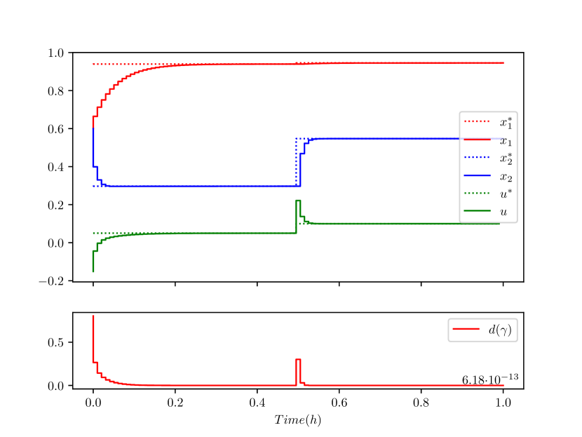
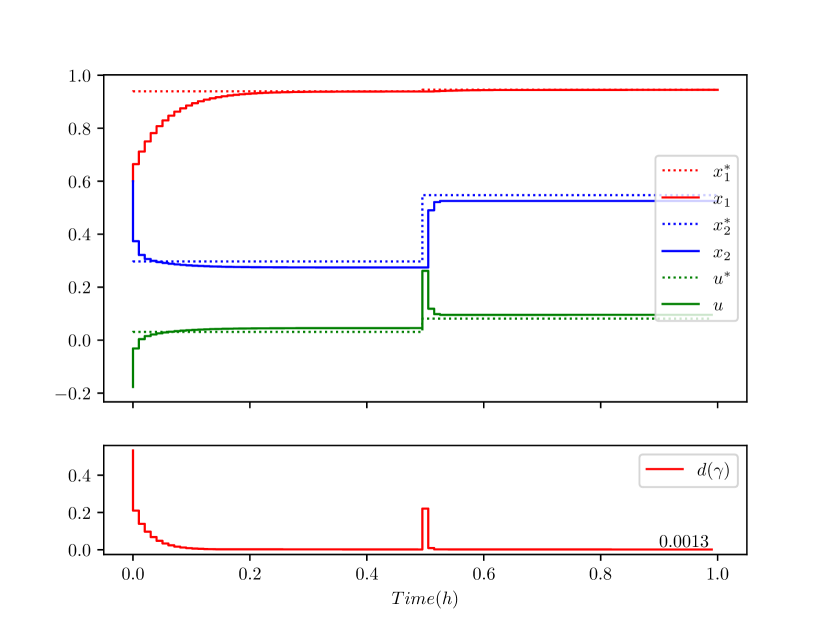
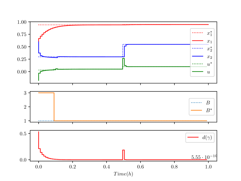
The CSTR was simulated using the proposed control design (as shown in Fig. 5) for the scenario when the reference generator uses the correct system parameter (hence, online learning is not required). Fig. 6 shows that when the exact model is known the discrete-time neural network embedded contraction-based controller (19) is capable of offset-free tracking. The system was then simulated with incorrect value of (with ), and without online parameter learning. Fig. 7 shows that bounded tracking was achieved as per Lemma 1 (observe that the Riemannian geodesic distance, , converges to a non-zero value comparatively), whereby the incorrect control reference generated using the incorrect value for caused the tracking offsets (see Section III-C). To further demonstrate the overall control approach, the same incorrectly modeled system was then simulated with the online parameter estimation module active from time . As shown in Fig. 8, the proposed approach achieved bounded reference tracking (as per Lemma 1) when parametric uncertainty was present (see ), and after the online parameter learning algorithm converged, offset free tracking (see also ) was achieved as per Corollary 1.
VI Conclusion
In this article, a framework was developed to train a DCCM neural network (contraction metric and feedback gain) for contraction analysis and control using a nonlinear system model with parametric uncertainties. Considerations were made for the discrete-time contraction and stability for certain nonlinear systems, which for known bounds on modeling uncertainty, were then extended to provide direct analysis and controller synthesis tools for the contraction of uncertain nonlinear systems. An online parameter “safe” learning module was also included into the control-loop to facilitate correct reference generation and consequently offset-free tracking. The resulting contraction-based controller, which embeds the trained DCCM neural network, was shown capable of achieving efficient tracking of time-varying references, for the full range of model uncertainty, without the need for controller structure redesign.
References
- [1] C. Zhang, Z. Shao, X. Chen, X. Gu, L. Feng, and L. T. Biegler, “Optimal flowsheet configuration of a polymerization process with embedded molecular weight distributions,” AIChE Journal, vol. 62, no. 1, pp. 131–145, 2016.
- [2] N. N. Chokshi and D. C. McFarlane, “DRPC: Distributed reconfigurable process control,” A Distributed Coordination Approach to Reconfigurable Process Control, pp. 43–49, 2008.
- [3] I. R. Manchester and J.-J. E. Slotine, “Control contraction metrics: Convex and intrinsic criteria for nonlinear feedback design,” IEEE Transactions on Automatic Control, vol. 62, no. 6, pp. 3046–3053, 2017.
- [4] W. Lohmiller and J.-J. E. Slotine, “On contraction analysis for non-linear systems,” Automatica, vol. 34, no. 6, pp. 683–696, 1998.
- [5] R. McCloy and J. Bao, “Contraction-based control of switched nonlinear systems using dwell times and switched contraction metrics,” IEEE Control Systems Letters, vol. 6, pp. 1382–1387, 2022.
- [6] R. McCloy, R. Wang, and J. Bao, “Differential dissipativity based distributed MPC for flexible operation of nonlinear plantwide systems,” Journal of Process Control, vol. 97, pp. 45–58, 2021.
- [7] S.-L. Dai, C. Wang, and M. Wang, “Dynamic learning from adaptive neural network control of a class of nonaffine nonlinear systems,” IEEE Transactions on Neural Networks and Learning Systems, vol. 25, no. 1, pp. 111–123, 2013.
- [8] W. He, Y. Chen, and Z. Yin, “Adaptive neural network control of an uncertain robot with full-state constraints,” IEEE Transactions on Cybernetics, vol. 46, no. 3, pp. 620–629, 2016.
- [9] H. D. Patino and D. Liu, “Neural network-based model reference adaptive control system,” IEEE Transactions on Systems, Man, and Cybernetics, Part B (Cybernetics), vol. 30, no. 1, pp. 198–204, 2000.
- [10] T. Wang, H. Gao, and J. Qiu, “A combined adaptive neural network and nonlinear model predictive control for multirate networked industrial process control,” IEEE Transactions on Neural Networks and Learning Systems, vol. 27, no. 2, pp. 416–425, 2015.
- [11] S. S. Ge, C. C. Hang, T. H. Lee, and T. Zhang, Stable Adaptive Neural Network Control. Springer, 2013, vol. 13.
- [12] D. Sheng and G. Fazekas, “A feature learning Siamese model for intelligent control of the dynamic range compressor,” in International Joint Conference on Neural Networks (IJCNN), 2019, pp. 1–8.
- [13] G. Leitmann, “On one approach to the control of uncertain systems,” Journal of Dynamic Systems, Measurement, and Control, vol. 115, no. 2B, pp. 373–380, 1993.
- [14] J. Shin, T. A. Badgwell, K.-H. Liu, and J. H. Lee, “Reinforcement learning–overview of recent progress and implications for process control,” Computers & Chemical Engineering, vol. 127, pp. 282–294, 2019.
- [15] M. Črepinšek, S.-H. Liu, and M. Mernik, “Exploration and exploitation in evolutionary algorithms: A survey,” ACM computing surveys (CSUR), vol. 45, no. 3, pp. 1–33, 2013.
- [16] M. do Carmo, Riemannian Geometry. Birkhäuser, 1992.
- [17] L. Wei, R. McCloy, and J. Bao, “Control contraction metric synthesis for discrete-time nonlinear systems,” in 11th IFAC Symposium on Advanced Control of Chemical Processes (Keynote Presentation), 2021.
- [18] Q.-C. Pham, N. Tabareau, and J.-J. Slotine, “A contraction theory approach to stochastic incremental stability,” IEEE Transactions on Automatic Control, vol. 54, no. 4, pp. 816–820, 2009.
- [19] R. Wang and J. Bao, “Distributed plantwide control based on differential dissipativity,” International Journal of Robust and Nonlinear Control, vol. 27, no. 13, pp. 2253–2274, 2017.
- [20] F. Schroff, D. Kalenichenko, and J. Philbin, “FaceNet: A unified embedding for face recognition and clustering,” in Conference on Computer Vision and Pattern Recognition, 2015, pp. 815–823.
- [21] D. P. Bertsekas, “On penalty and multiplier methods for constrained minimization,” SIAM Journal on Control and Optimization, vol. 14, no. 2, pp. 216–235, 1976.
- [22] P. Molchanov, S. Tyree, T. Karras, T. Aila, and J. Kautz, “Pruning convolutional neural networks for resource efficient inference,” in 5th International Conference on Learning Representations, ICLR 2017-Conference Track Proceedings, 2019.
- [23] S. P. Boyd and L. Vandenberghe, Convex optimization. Cambridge University Press, 2004.
- [24] B. J. Taylor, Methods and Procedures for the Verification and Validation of Artificial Neural Networks. Springer, 2006.
- [25] M. A. Armstrong, Basic Topology. Springer, 2013.
- [26] A. Olivier and A. W. Smyth, “On the performance of online parameter estimation algorithms in systems with various identifiability properties,” Frontiers in Built Environment, vol. 3, p. 14, 2017.