Discrete Search in Heterogeneous Integer Spaces for Automated Choice of Parameters using Correct-by-Construction Methods

Discrete Search of integer spaces provides a powerful mechanism through which to explore the reachable set of a given system. Current design cools work primarily for homogeneous parameter spaces, and mapping a heterogeneous parameter space into the integer domain would provide a strong backbone for both performance and allow for a wide range of uses in many hybrid systems as well as hybrid parameters that are contained within a single system. There are precautions that would need to be taken for hybrid systems, which primarily consist of having unsafe states, that even though they are reachable, they would be considered to be unsafe in a real-world implementation, as well dependencies between variables, that could transcend the homogeneous dependencies that are trivial (i.e. comparing two integers together as compared to a comparison between floating point and Boolean). There also would exist optimal state locations of the parameter set, and those would be modeled using an arbitrary cost function.

Related work consists primarily of homogeneous tool parameter exploration implementations, and those concern themselves primarily with arriving at the reachable set primarily for homogeneous parameter sets. This would include the tool Ariadne [1], which has features built-in that allow it to find an approximation of the given reachable set by giving by controlling the growth of the approximation error.

One other concern that arises when attempting to model heterogeneous parameters in integer spaces is the problem of solvability within bounded time with close approximation, and as outlined in [2], there does exist a finite bound for finite discovery. There was a foray into unbounded analysis, but that is infeasible given the constraints and would be too computationally exhaustive. Another issue that comes up is discrete versus non-discrete evolution in terms of time, and this was a problem resolved by setting as a condition that there can only exist discrete time steps and discrete evolution.

For the implementation demonstrated in this paper, we focus on a number of contributions that create a fast and efficient method of finding the optimal set given existing constraints and cost. We also define a semantic format that supports the representation of heterogeneous parameters, which better suits it for discrete search along hybrid domains.

For exploring the adjacent set space from our beginning iteration point(initial state), there are a number of possible implementation decisions that would need to be made on how best to explore the reachable set given the constraints. The path that we decided on was to create a correct by construction approach, that would allow the exploration tool to only explore the reachable set that is also valid given the constraints and dependencies that are supplied. Our flow is as follows: given a parameter list which can consist of integer, Boolean, and composite parameters, as well as a list of constraints and dependencies between variables, and a cost function, we aim to find a valid parameter state that satisfies all of our given requirements.

For our implementation, we split our computational engine into two general algorithms. Our first algorithm involves computing a correct-by-construction interval for a given parameter given our requirements, and our current state when it comes to other parameters that exist within our set space. The second algorithm is our step-by-step evolution iteration across the set space of the parameter list based on the computation of local optimal cost.

Compared to existing and related works, our approach has the following contributions:

• •

  Developed a representation for heterogeneous parameter sets that allows for the discretization of all parameters and results in the ability for integer space exploration for all relevant types

• •

  Created a correct-by-construction approach to not only finding the reachable set of a given parameter set, but also allowing the inclusion of heterogeneous inter-parameter dependencies and assertions.

• •

  Designed a method of evolution that allows for quick computation of adjacent states for a given set of already locally-optimal parameter instances with a method of back-tracing and reset if arriving at an invalid location

• •

  Demonstrate the applicability and the versatility of our implementation on two examples that involve computing minimum cost for a computer architecture design and a re-programmable logic circuit with a demonstration of the implementation of pseudo-Boolean constraints

We decided on implementing our design in Python[4], the reason for that being that Python allows a host of libraries and type-interfacing that would allow us to quickly prototype, verify, and extend during testing. We also chose Python for the reason of being able to interface easily with JSON[5], which is our input-format of choice. JSON was chosen due to its status as being very well-adopted and would provide an easy interface for other CAD tools to create tool-parameter sets for analysis using our program.

We also use a number of Python libraries to do the necessary computations that are required for our implementation. A special recognition is deserved of Numpy[6], which is a library that allows for very quick computation of intervals, arrays, and sets. Since we are operating in the integer domain, integer arrays using Numpy libraries make the cost of computation a significantly smaller area of concern during implementation.

To better improve the performance of discrete search in heterogeneous space, there do exist a number of limitations. Firstly, a slight weakness exists in parsing string type assertions and evaluating them in a computationally static format as opposed to extensive abstract syntax trees and symbolic interval computation. Secondly, considering various typed parameters and assertion relations, it is necessary to have a uniform interface design such that algorithm implementation is isolated with complicated typed transformation, which is why JSON was selected, which could become unwieldy if enumerated or vector parameters which to be considered. In this case, a tool that would generate a statically-enumerated JSON format that is acceptable to our program would be required.

In this section, we introduce how the program will explore feasible set constrained by assertions. The JSON format input will be interpreted and loaded into our program. For the sake of generality, we assume that there are $n$ parameters denoted as $x_{1},\cdots x_{n}$. First of all, for each parameter $x_{i}$, we randomly generate $N-1$ valid neighboring points. For the random sampling of these points, we experimented with a couple methods. One was uniform sampling from the valid interval, the other two where linear and square weighted sampling with respect of distance from the interval. After these were tested, we found that square weighting was the most effective, and we will demonstrate these findings during our examples. With $x_{i}$ itself, these $N$ points form a list $\{x_{i}^{j}\}_{j=1}^{N}$. In total there are $n$ lists.

During the evolution process, each point will randomly generate a neighboring point from its valid set. Therefore, all $n\cdot N$ points will generate another $n$ new lists. Without loss of generality, we denote these $n$ new lists as $\{x_{i}^{j}\}_{j=N+1}^{2N}$. Next we the original list and new list with the same footnote $i$ to get $n$ new list $\{x_{i}^{j}\}_{j=1}^{2N}$. From these $n$ list, we evaluate $2N$ cost function values as $\{c_{j}=F(x_{1}^{j},x_{2}^{j},\cdots x_{n}^{j})\mid j=1,\cdots,2N\}$. For these $2N$ cost values, we keep the smaller half and corresponding parameter values to form $n$ new lists. Repeat the above steps until the ending requirements are satisfied. A pseudo-code for this algorithm can be found at Algorithm 1

For defining the the set of parameters that would exist for a given system, we supply two atomic types and one composite type:

1. 1.

   Integer type

2. 2.

   Boolean type

3. 3.

   Composite type

Integers exist in the Integer domain, and Boolean’s likewise in the Boolean domain. Composites are different in that they are modeled like an array, given a composite parameter $C$, $C$ can contain any number of composites, Boolean’s, and integers. This allows the modeling of parameters that cannot be modeled as strictly scalar integer or Boolean values. Floats, complex numbers, and vectors are all examples of what can be modeled as a composite set. Furthermore, to maintain the desired behavior of these parameters, the constraint paradigm that we introduce allows us to describe the behavior of how these composite parameters undergo evolution.

As an example, take $Cube$, which of type composite, and it is defined by 3-equal length sides $x,y,z$, such that $Cube(t)=\{x,y,z\in\mathbb{Z},x==y==z\}\forall t$ where $t$ is time-step during evolution. For the case of this parameter, the instantiation of the of the domain of each sub-parameter would go with the parameter declarations, while the instantiation of the constraint that is intrinsic to cubes would be added to the constraints field that is given.

This paradigm of allowing composite parameters to have unique behaviors could lead to invalid states during evolution, if one sub-parameter undergoes evolution independently and is now not equal to the other two, that would lead to an undesirable state. For this reason correct-by-construction interval generation for each of the sub-parameters is done with all assertions and constraints in mind.

One note on using composite parameters to model floating point numbers. Initially during development we had planned to incorporate a floating point type, however the tediousness of setting properties for floating point as an atomic type is redundant as all the properties of a floating point value(mantissa, exponent, significant figures) can be modeled as sub-parameters of a composite value, and the user can specify the desired constraints and behaviors for comparison and incorporation between the composite-ized floating point value and other parameters.

In this section, a detailed explanation about how to construct valid neighboring set is given. Suppose that there are $m$ assertions $\{\mathcal{A}_{i}\}_{i=1}^{m}$ on $n$ parameters. For each parameter $x_{i}$, assertions containing $x_{i}$ are selected out of $m$, which is $\{\mathcal{A}_{k}\mid x_{i}\in\mathcal{A}_{k}\}$. Next, iterate through other parameters and apply their values into these assertions. Finally, Intersect all the intervals after evaluating the assertions to get the final interval. A new value for $x_{i}$ is sampled randomly from the final interval based on the square of their distance to $x_{i}$. By default, values closer to $x_{i}$ have higher probabilities to be selected. More details can be found in Algorithm 2

One initial idea that was considered well thought out and feasible was the incorporation of symbolic computation for our constraint and dependency valid interval generation. The Sympy[7] library in Python was going to be utilized for this purpose. Though the algorithm was functional, the symbolic computation cost was extremely prohibitive, and was not feasible for a general-use case. After doing much research to attempt to make it feasible, we discovered that even Sympy as an organization recognizes that the substitution and evaluation is cost-prohibitive, and recommends other avenues for repetitive computation. For this reason we had to re-calibrate and find another solution. This solution was to do string replacement of our given parameters with their values into the string representation of our constraints, dependencies, and costs. Then these string representations would be converted into lambda functions that would be operated on by the Numpy array operations. Since Numpy on the back-end uses C libraries to do computation, this lessened our computation time by an order of magnitude, for mostly the same functionality.

The functionality that is missing is due to the inherent behavioral properties of lambda functions. Symbolic computation was desired as it allowed the incorporation of very rigorous Boolean SAT exploration, but this is not a feature that is possible with the lambda paradigm. Therefore, to allow the extend-ability of Boolean values, fuzzy pseudo-Boolean logic[8] is implemented, which does allow for an adequate semantic representation of Boolean logic.

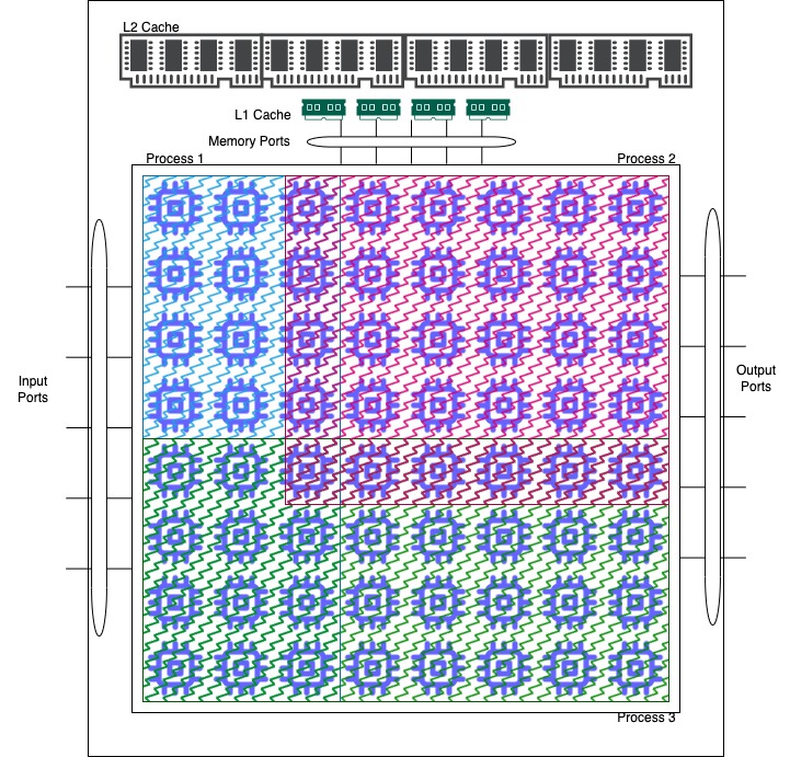
For our first example(outlined in 2), we decided on modeling our problem as an FPGA cost problem. Given a number of constraints on an FPGA, i.e. memory size, available memory ports, available input and output ports we have $Routine_{1,2,3}$, and only two of the previously mentioned three can be installed on the FPGA fabric, and depending on which two are loaded onto the fabric, we then must enable a minimum number of memory, I/O, and interconnection ports, as well as have different memory properties. We then created a polynomial cost function of these constraints, in an aim of it becoming nonlinear and make the algorithm demonstrate its effectiveness in traversing the set space while attempting to find the given most optimal cost.

One highlight of this example is the inclusion of pseudo-Boolean constraints, which manifest in the requirement that only two of the three routines can function at any time, which in terms of cost, creates a piece-wise function. The parameter variation that is generated during random sampling is able to traverse this piece wise function, because even though we generate points using a correct-by-construction approach, in some cases there is no valid interval, and in that case we reset for that specific parameter back to the largest valid interval, and randomly sample that. This allows the program to exit any possible rut that it enters while making an early decision on which Routine set to choose, and so it can backtrack as necessary and choose another Routine set if the specific parameter space undergoing evolution is no longer valid. The results for these are demonstrated in Figure 3 with different weights for random sampling methods from the valid intervals generated.

Another example that we used is the creation of of a computer architecture system. During the creation of a new computer architecture, or the generation of a new implementation of an architecture, multiple design decisions must be made with respect to area, inter-connectivity, interface requirements, and transistor count. In this example, we model a simple multi-fetch, multi-execution, processor design. We drafted the requirements in terms of dependencies and constraints, and given the constraints and requirements for the interfaces and inter-connectivity between components, we aim to find the minimal transistor count. This was a more rudimentary design, and it aimed to find the computation limit of our implementation. One thing that we attempted to model was having very large integer sets, and exploring those. Emulating design space exploration for computer architectures with such large intervals was the reason we had to refactor our computation engine from purely symbolic to the lambda paradigm, as the symbolic computation was not able to run search space exploration and computation in a reasonable amount of time with this example. The results for those example are posted in Figure 4, along with the variation between random sampling methods from the valid intervals generated.

As aforementioned during the discussion on the implementation, performance was a major bottleneck in our implementation, and there were a number of features that needed to be added to be able to guarantee reasonable performance. The first was the use of lambdas to calculate the valid interval set. The second, which is outlined in the algorithm, is keeping a short list of the least-cost neighbors that exist, and generating new random neighbors from that list. This allows us to have multiple different forays into the search space, and we could possibly arrive to many local minima’s, but we only choose the most optimal local minima. Computation time is static across iterations, and there are parameter options to increase or decrease the exhaustiveness of the search depending on the intended use cases.

We also wanted to verify the efficacy of our design and do the best possible effort into generating the most optimal point. To verify that our results where sane, we ran multiple different instances of both the FPGA and Computer Architecture description JSON files, and averaged those results out, and did this for three different weights for random sampling(uniform, linear weighted, square weighted), and what we found that in all cases, our results for all runs where fairly similar, but there are some noticeable differences worth discussion.

Firstly, the uniform random search has better performance for lower iterations, and this is because during early stages of evolution, a majority portion of the set space has yet to be explored, and uniform sampling allows us to traverse the majority of the set space early. However after a lot of iterations, the square weighted random sampling from the interval eventually makes us arrive to a more optimal cost, and this is because as more and more of the set space is invalidated, the parameters that are undergoing evolution get much closer to the local optima, and square weighting allows us to more likely sample these local optima and arrive at them at a quicker rate than both uniform and linear random sampling.

One feature that would have been useful to incorporate would have been incorporating a Boolean SAT or SMT solver[9], which would have allowed us to bypass pseudo-Boolean constraints entirely, which are generated heuristically, and instead rigorously solve Boolean equations for all possible solutions. Incorporation a Boolean SAT solver such as Z3 would’ve been time-prohibitive, but would’ve allowed for a greater range of expressively for constraints.

Due to space reasons, we do not go into detail on the specifics of the Computer Architecture Example and the FPGA Example. Please contact the authors for more information.

References

- [1] Luca Geretti, Pieter Collins, Davide Bresolin, and Tiziano Villa. Automating numerical parameters along the evolution of a nonlinear system. In Runtime Verification: 22nd International Conference, RV 2022, Tbilisi, Georgia, September 28–30, 2022, Proceedings, page 336–345, Berlin, Heidelberg, 2022. Springer-Verlag.
- [2] Michele Conforti, Gerard Cornuejols, and Giacomo Zambelli. Integer Programming / Michele Conforti, Gérard Cornuéjols, Giacomo Zambelli. Springer, Cham, 2014.
- [3] Ian M. Mitchell and Claire J. Tomlin. Overapproximating reachable sets by hamilton-jacobi projections. Journal of Scientific Computing, 19(1):323–346, 2003.
- [4] Guido Van Rossum and Fred L Drake Jr. Python reference manual. Centrum voor Wiskunde en Informatica Amsterdam, 1995.
- [5] Felipe Pezoa, Juan L Reutter, Fernando Suarez, Martín Ugarte, and Domagoj Vrgoč. Foundations of json schema. In Proceedings of the 25th International Conference on World Wide Web, pages 263–273. International World Wide Web Conferences Steering Committee, 2016.
- [6] Charles R. Harris, K. Jarrod Millman, Stéfan J. van der Walt, Ralf Gommers, Pauli Virtanen, David Cournapeau, Eric Wieser, Julian Taylor, Sebastian Berg, Nathaniel J. Smith, Robert Kern, Matti Picus, Stephan Hoyer, Marten H. van Kerkwijk, Matthew Brett, Allan Haldane, Jaime Fernández del Río, Mark Wiebe, Pearu Peterson, Pierre Gérard-Marchant, Kevin Sheppard, Tyler Reddy, Warren Weckesser, Hameer Abbasi, Christoph Gohlke, and Travis E. Oliphant. Array programming with NumPy. Nature, 585(7825):357–362, September 2020.
- [7] Sympy Foundation.
- [8] Y. Dote. Introduction to fuzzy logic. In Proceedings of IECON ’95 - 21st Annual Conference on IEEE Industrial Electronics, volume 1, pages 50–56 vol.1, 1995.
- [9] Leonardo De Moura and Nikolaj Bjørner. Satisfiability modulo theories: Introduction and applications. Commun. ACM, 54(9):69–77, sep 2011.